Detection of contaminants using a MEMS FAIMS sensor

Detection of Contaminants

Using a MEMS FAIMS Sensor

by

Kristin Carr

Submitted to the Department of Electrical Engineering and Computer Science in partial fulfillment of the requirements for the degree of Master of Engineering in Electrical Engineering and Computer Science

at the

MASSACHUSETTS INSTITUTE OF TECHNOLOGY

1Vay 2005

@ Copyright 2005 Kristin Carr. All rights reserved.

The author hereby grants to M.I.T. permission to reproduce and distribute publicly paper and electronic copies of this thesis

and to grant others the right to do so.

Author

Department of Electrical Engineering and Computer Science May 19, 2005 Certified by Certified by_ Accepted by

D

h ulGreenberg, Ph.D. .MI.T esis Advisor

Arthur C. Smith Chairman, Department Committee on Graduate Theses

OF TECHNOLOGY

AUG

14

2006

Detection of Contaminants

Using a MEMS FAIMS Sensor

by Kristin Carr

Submitted to the Department of Electrical Engineering and Computer Science

May 19, 2005

In partial fulfillment of the requirements for the degree of Master of Engineering in Electrical Engineering and Computer Science

Abstract

Detecting the presence of contaminants in water is a critical mission, but thorough testing often requires extensive time at a remote facility. A MEMS implementation of a FAIMS (High-Field Asymmetric-Waveform Ion Mobility Spectrometry) sensor has recently been developed, and is capable of promptly analyzing water on-site. In this thesis, we apply two well-established statistical target detector algorithms to the detec-tion of chlorite in water. The matched filter and the adaptive cosine estimator (ACE) are subspace detectors that possess complimentary geometric properties. We address several significant challenges in implementing these detectors, including the estimation of the covariance given the limited amount of data available and the design of a target signature subspace in response to the fact that the signature does not scale linearly with the contaminant concentration. In addition, we consider the need for dimension reduc-tion through the use of wavelets. We evaluate each of the detectors on FAIMS data of pure and chlorite-contaminated water.

Draper Thesis Advisor: Nirmal Keshava, Ph.D. Title: Principal Member of Technical Staff

M.I.T. Faculty Thesis Advisor: Julie Greenberg, Ph.D. Title: Principal Research Scientist

Acknowledgements

May 19, 2005

I would like to thank everybody at Draper Laboratory for their help on the work presented in this thesis. I would like to specifically thank the biomedical engineering group for their work in developing the FAIMS sensor and all of the data acquisition techniques documented in this paper. Cristina Davis, Melissa Krebs and Julie Zeskind were responsible for the idea of water analysis using FAIMS. Heather Clark and Marianna Shnayderman were critical in the testing and development of the FAIMS instruments and were very helpful in their immense assistance in data acquisition. In addition, there were many people who helped in collecting data, developing

instrumentation techniques, teaching and explaining FAIMS and biological concepts, and being willing to discuss ideas and research paths. These include those individuals named above, in addition to Angela Zapata, Sarah Cohen, Will Merrick, Daniel Traviglia.

I am also grateful for the guidance, support, knowledge, and patience of Nirmal Keshava, Melissa Krebs, Cristina Davis and Heidi Perry, and my advsior, Julie Greenberg, all of without whom this thesis would not be possible.

This thesis was prepared at The Charles Stark Draper Laboratory, Inc., under Internal Research and Development Project Number 12591-001.

Publication of this thesis does not constitute approval by Draper or the sponsoring agency of the findings or conclusions contained herein. It is published for the exchange and stimulation of ideas.

Contents

1 Introduction 11

1.1 Background and Motivation . .. . . . . 11

1.2 Project Overview . . . .. . . . . 12 1.3 Related Works. . . . . 13 2 FAIMS 15 2.1 Description . . . . 15 2.2 Sample Introduction . . . . 18 2.3 Sensor Quantization . . . . 18 2.4 Signal Model . . . . 20 3 Data Acquisition 23 3.1 Overview . . . . 23

3.2 FAIMS Setup & Parameters . . . . 23

3.3 Detector Implementation . . . . 25

3.4 Data Description . . . . 25

4 Problem Formulation and Development 29 4.1 Problem Description . . . . 29

4.2 Bayesian Derivation . . . . 29

5 Noise Analysis 33 5.1 Overview of Analysis and Estimation . . . . 33

5.2 Covariance in Time . . . . 34

5.3 Covariance in Vc . . . . 35

5.4 Histograms . . . . 36

6 Matched Filter and ACE Detectors 39 6.1 Matched Filter . . . . 39

6.1.1 Overview . . . . 39

6.1.2 Assumptions . . . . 40

6.1.3 Implementation . . . .. . 40

6.2 Adaptive Cosine Estimator . . . . 40

6.2.1 Overview . . . . 40

6.2.2 Assumptions . . . . 41

6.2.3 Implementation . . . . 41

6.3 Performance Metrics . . . . 41

6.4 Results . . . . 43

7 Multidimensional Target Subspaces 49 7.1 Overview & Motivation . . . . 49

8 Wavelet Transform & Associated Detectors 57

8.1 Overview & Motivation . . . . 57

8.2 Implementation . . . . 58

8.3 Associated Matched Filter & ACE Detectors . . . . 59

8.4 R esults . . . . 60

9 Conclusion 67 9.1 Sum m ary . . . . 67

List of Figures

1 FAIMS schematic & ion flow path [1] . . . . 15

2 ERF(t): FAIMS asymmetric electric field [1] ... ... 16

3 FAIMS force directions [1] ... ... 16

4 Histogram of noise points illustrating sensor quantization . . . . 19

5 Top-View Plots of FAIMS Spectra for Water and Chlorite-Contaminated Water at 2.5 ppm and 40 ppm . . . . 27

6 Covariance in V (mesh view) . . . . 35

7 Covariance in V (top view) . . . . 35

8 Covariance in time (mesh view) . . . . 36

9 Covariance in time (top view) . . . . 36

10 Histogram of noise with fitted Gaussian probability distribution function 37 11 ACE detector output (AACE) statistics (ptrain=2.5 ppm) . . . . 44

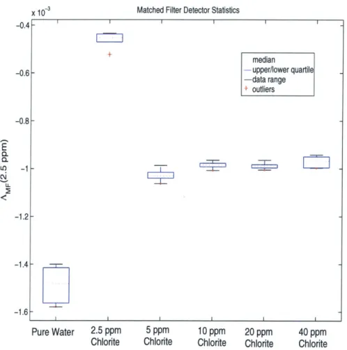
12 Matched filter detector output (AMF) Statistics (pitrain=2.5 ppm) . . . . 45

13 y for matched filter and ACE detector (itrain=2.5 ppm) . . . . 46

14 - for ACE detector at all testing and training concentrations . . . . 47

15 y for matched filter detector at all testing and training concentrations . . 48

16 Mean energy for chlorite . . . . 49

17 Angle between concentrations . . . . 49

18 y for matched filter and ACE multidimensional subspace detectors . . . . 53

19 y for multidimensional subspace detectors as compared to best and worst case single dimensional detectors . . . . 54

20 Percentage of energy retained versus number of coefficients retained after wavelet transform . . . . 60

21 Wavelet transform matched filter detector statistics (ptrin=2.5ppm, 6 coefficients retained) . . . . 61

22 Wavelet transform ACE detector statistics (Ptrain=2.5 ppm, 6 coefficients retained) . . . . 62

23 -y for matched filter wavelet transform detector at 6 different coefficient levels and all testing concentrations . . . . 63

24 -y for raw and wavelet transform detectors with 6 coefficients retained (p est= 2.5 ppm ) . . . . 64

List of Tables

1 Headspace sampler parameters . . . . 24 2 G C param eters . . . . 24 3 FAIMS parameters . . . . 24 4 -y for matched filter & ACE multidimensional detectors (MF/ACE) . . . 55

1

Introduction

1.1

Background and Motivation

The ability to accurately determine the safety level and contaminant concentration of water is critical, but thorough testing often requires extensive time and sophisticated facilities for chemical tests to be run a great distance away from where the water sample was taken [15]. This serves as the motivation for an on-site water monitoring tool through which water can be sampled and then processed by a statistical detector to give an indication of the presence or lack of contaminants in the water.

The FAIMS (High-Field Asymmetric-Waveform Ion Mobility Spectrometry) sensor is a recently-developed analytical sensor that has been used to measure and analyze ion mobility properties of biological and chemical materials [16, 17, 18, 19, 20, 21, 22, 26, 27]. It can be used to analyze water samples, and does not require the addition of any chem-ical reagents nor extensive handling and processing of the sample that many other water monitoring methods require [15]. Further, a MEMS (Micro-Electro-Mechanical System) device has been developed at Draper Laboratories to analyze samples and produce a pair of three-dimensional signals indicative of the concentration levels of different types of ions in the sample [1, 16].

Because the spectrometer has been implemented in a MEMS device, it can poten-tially be used to acquire and analyze water samples at the site as a small, portable device capable of almost instantly determining water safety levels. Researchers at Draper Lab-oratory have previously acquired data demonstrating the ability of FAIMS to detect changes in water quality and the presence of contaminants [37]; however, the initial study only provided the basis of proof-of-concept classification of signals evaluated post-acquisition. The primary objective of this thesis is to introduce and develop analytical techniques for the statistical detection of contaminants in water using FAIMS with the

of detection (PD).

1.2

Project Overview

This thesis aims to develop and evaluate several advanced methods for the detec-tion of contaminants in water using FAIMS. We employ techniques well-established on other types of data and examine their application to the FAIMS data. With a goal of minimizing the error rate of the detector, we devise an optimal strategy assuming an infinite quantity of FAIMS pure and contaminated water data for use in real-time analysis. Given our limited number of data samples and a desire for low computational requirements, we examine the various assumptions that allow us to proceed to a series of different statistical analysis methods, hereafter referred to as detectors. Note that the term "detector" will be used in this thesis to refer to the statistical detection algorithm implemented in software as the step following FAIMS data acquisition; this term will not be used to refer to the FAIMS hardware.

We analyze and evaluate two complimentary subspace detectors: a matched filter detector [9], which is based on the relative energy' in the received signal, and an adaptive cosine estimate (ACE) detector [9], which is based on the relative angle in the received signal. Both are based upon a linear signal model and Gaussian additive noise, and have been derived to be statistically optimal for distinct signal models. ACE also has the desirable property of maintaining a constant false alarm probability (CFAR) under certain variations in the noise model.

We also consider the case of a multi-dimensional target subspace for both the matched filter and ACE detectors. This will be relevant if the target signals span a multidimen-sional subspace as they vary with concentration instead of simply increasing in mag-nitude [9]. Algorithms developed for radar data have been employed to detect radar target signatures for the conditions and environments in which radar systems operate.

Although FAIMS collects data in a significantly different environment, our goal is to investigate how well contaminants (i.e., targets) can be modeled and detected under the same assumptions.

In addition, we employ a wavelet transform [10] to reduce the dimensionality of the original data and thus improve the covariance estimates on a smaller number of coefficients. We then implement the corresponding matched filter and ACE detectors on a limited number of those wavelet coefficients.

In order to properly juxtapose the different detector performances, we create a metric based on the level of separation between classes yielded by each of the detectors. Without enough data to sufficiently generate a receiver operating curve (ROC), this metric allows us to compare detectors for the purpose of minimizing the rate of error. A more rigorous analysis of detector outputs would utilize the exact parametric form of the detector test statistic, but requires significantly more experimental data than was at our disposal.

1.3

Related Works

There has been no published work using a statistical detector with FAIMS sensor data to detect contaminants in water. The few related papers utilize the FAIMS technology, but concentrate on results that visually discern different ion species [14, 18, 19, 20, 21, 23, 26] and do not employ any statistically optimal approaches. In addition, because FAIMS can be used in a variety of different setups (e.g., using a different sensor or sample introduction technique), there is a vast array of FAIMS data that is very different, and yields different types of datasets indicative of different quantities [12, 13, 19, 20, 27, 29, 30]. As a result, the processing required on such datasets is different.

Despite the lack of published results involving statistical detectors on FAIMS data, the field of classification and detection is rich in similar work done on other types of data. These papers include the development and evaluation of a large class of subspace

[9], both of which will be utilized in this thesis [35, 36].

We address the notion of a wavelet transform to gain parsimonious representations of FAIMS data; this concept as applied to other types of data is one which has been widely publicized [10, 11, 31, 32, 33, 34]. We will draw on these concepts as the building blocks for the wavelet section of this thesis.

2

FAIMS

2.1

Description

The technology in use is a FAIMS sensor which measures the abundance of ions arriving at the sensor after travelling through a channel with an externally applied electric field. Conventional ion mobility spectrometers operate in the low field regime where the applied electric field strength is less than 1000 V/cm and the mobility is essentially constant [1]. However, it has been demonstrated that the mobility of an ion is field dependent and can change significantly as the field strength increases [2].

Different ion species will have particular mobility dependencies on an electric field, and the FAIMS technology utilizes this differential mobility of ions in an electric field to identify the different ion species.

ionization

O

Source RF electric field

Sample~

in Gas ,Detector

Flow'

Eecpc field adjusted to aDow this

-Comipensation _{ion species to pass trough to}

Ion Trajectonies electric field detector

Figure 1: FAIMS schematic & ion flow path [1]

The FAIMS sensor operates as follows: a gas sample derived from the headspace above a water sample (described in Section 2.2) is introduced to the FAIMS spectrometer; after entering the spectrometer, the ions are transported by a carrier gas between a pair of parallel plates in which an asymmetric electric field, ERF(t), is applied at radio

the parallel plates, and a sensors at the end of the plates measure the voltages resulting from the stream of positive and negative ions arriving at the sensors. The electric field alternates at radio frequencies with an asymmetric duty cycle between a high-magnitude positive electric field (Emax) and a low-magnitude negative electric field (Emin) so that the net electric field is zero, as shown in Figure 2 [1].

ER (t)

E iax

.

...

E

_

't

Figure 2: ERF(t): _{FAIMS asymmetric electric field [1]}

To better understand how the FAIMS technology works, we can consider the forces that act on a single ion. The ion experiences a constant force from the carrier gas flow (z-directed) which transports it through the parallel plates.

YV

L

Z Gas Flow

Figure 3: FAIMS force directions [1]

A transverse force (y-directed), produced by the RF electric field (ERF(t)) and a DC compensation voltage (V), also acts on the ion, as shown in Figure 3 [1]. These fields are generated by applying voltages to the parallel plate electrodes. The resulting ion

velocity in the y-direction is given by [3]:

V, = KE ₍₁₎

where K is the coefficient of ion mobility for the ion species and E is the electric field in-tensity. The dependence of the mobility on the electric field intensity can be represented by the following expression [3, 4]:

K(E) = KO[I + a2E2 + a4E4 + ... (2)

where a2 and a4 are coefficients of a series expansion, and KO is the mobility coefficient in

a vanishingly small field [6]. As the electric field strength increases (above 5000 V/cm), the second and higher order terms in the series become significant and the mobility coefficient can change substantially (10-15%) from its low field value.

If we take K1 to be the mobility of a particular ion at Emax and K2 to be the

mobility of the ion at Emsi, then the average displacement of the ion in the y-direction as a function of time can be expressed as [1]:

y(t) = 3(K1 - K2) * t (3)

where / is a constant determined by the strength and duty cycle of the applied electric field. Thus, the overall trajectory will not be straight if the mobilities K1 and K2 are

not equal. To compensate for this and to allow the ion to arrive at the sensor, a low-field compensation electric field can be applied to the parallel plates.

A range of compensation voltages is repeatedly swept through linearly for each time sample, and the positive and negative sensors measure the voltage generated at the detector for each particular compensation voltage at each time sample, which yield a quantification of ions present. The ions strike a Faraday plate which generates a

generated by both the positive ions and the negative ions, and this voltage is referred to as the ion abudance or ion intensity value for each point in time and compensation voltage. The resulting output of the FAIMS sensor is a pair (one for each polarity) of three-dimensional signals of ion intensity that are dependent on the time, t, and compensation voltage V.

2.2

Sample Introduction

The FAIMS setup discussed above requires specialized sample introduction and ion-ization methods. The data used in this thesis was taken with a headspace sampler and used gas chromatograph (GC) as a pre-separation step prior to the gas sample entering the FAIMS unit. The headspace sampler heats up the given fluid sample, which has the effect of transferring substances that are volatile at that temperature into the air in the sample vial above the water. The headspace sampler then removes a sample of the air

in the vial and GC is used to provide a separation in time of the substances presented to the FAIMS unit. When the substance enters the FAIMS device, the material is ionized using a beta-particle emitting radioactive nickel source (63 Ni).

The motivation behind this comes from the fact that we are interested specifically in detecting chlorite; since chlorite is a particularly volatile substance, 63

Ni is well suited to ionizing the analyte. The initial headspace gas chromotograph (HS-GC) separation yields a first pass at extracting the substance of interest, thus yielding a higher ratio of contaminant signal to water background.

2.3

Sensor Quantization

There are limitations on the analog-to-digital converter attached to the FAlMS sensor that converts the analog voltage values into a digital output as read in by accompanying software. As a result, the sensor output is quantized to discrete values. This sets an upper bound on the level of resolution, which is empirically found to be approximately 10

uV. Figure 4 shows a histogram of points from the entire collection of pure and chlorite-contaminated data samples. This figure illustrates the fraction of data points that fell into each range of ion intensity values. The ionization intensity range was divided into sections, or "bins", 2 IV wide, and the histogram shows the fraction of the data fell into each section. As can be seen in Figure 4, there are many empty bins between each full bin; this indicates that the ion intensity values do not exist in a continuum, but instead have been quantized to discrete intervals. This can lower the overall performance of the data analysis methods and is one of the sources of noise that we will analyze in subsequent chapters. .18 .15 (D 0 C .12 0 40 0 >~.09 Cr 06 L. .03 0 0.02 0.03 0.04 0.05 0.06 0.07 0.08 0.09 0.10 0.11 0.12 Ion Intensity (mV)

2.4

Signal Model

In order to properly develop a statistical detector, it is necessary to model the received signal. Toward this end, we develop a signal model to describe the process that results in the measured signal from the FAIMS sensor.

The water sample without contamination possesses a characteristic background sig-nal, and we model the contaminated water as the sum of the background water signal with an additional signal due to the contamination. This model assumes linearity in the addition of the water background and contaminant signals.

The received signal is dependent on the contaminant type, concentration level, Emax and Emin (the high and low electric field magnitudes), and the background water source. In its most general form, the received 3-dimensional positive and negative ion signals will be:

r(t, V) =

f

where r, the received signal, is the voltage (mV) measured at the FAIMS sensor, and t and V are the time (seconds) and compensation voltage (V), respectively, at which the voltage was measured. The signal, n(t, V), is the random additive noise accounting for the variation in the signal that we model as Gaussian and will examine further in section 5.

If we do not vary Emax, Emin and the deionized water source, as is the case in this

project, we can simplify this to:

r(t, V) = f (contaminant, concentration) + n(t, V) (5)

If we assume that the ion quantities in the contaminated sample add linearly to the background, then the function

f

r(t, V) = s(t, V) + w(t, V) + n(t, V) (6)

Thus, in the context of a statistical detector to differentiate between the hypotheses

HO and H1, we have the binary hypothesis test:

Ho : ro(t, V) = w(t, V) + n(t, V) (7)

H, : ri(t, V) = s(t, V) + w(t, V) + n(t, Vc) (8)

where the signals ro and r1 correspond to the received signals under the null hypothesis

3

Data Acquisition

3.1

Overview

We focus on chlorite as the contaminant used in the training and testing of a suitable statistical detector algorithm. Concentrations of 2.5 ppm, 5 ppm, 10 ppm, 20 ppm, and 40 ppm of chlorite-contaminated water, in addition to pure water, were submitted to the FAIMS sensor and used as training and testing data.

The contaminated samples were obtained by mixing deionized water with household bleach (5.25 % NaClO). 152 pL of bleach was mixed with 199.848 mL of deionized water to obtain 200 mL of a chlorite-contaminated solution with a concentration of 40 ppm. Half of this solution was removed and added to 100 mL of deionized water to obtain 200 ml of a chlorite-contaminated solution with a concentration of 20 ppm. This process was repeated to obtain new solutions with half the concentration of the previous solution until the lowest concentration of 2.5 ppm had been created.

A total of 76 vials were created, with each 20 mL vial containing 10 mL of pure or contaminated water. The 76 vials were comprised of 16 pure water samples and 12 samples of each concentration of the chlorite-contaminated water. The vials were were split over two runs (with 38 samples each). A total of 76 data files were obtained, with 16 pure water samples, and 12 samples of each concentration of chlorite solution.

3.2

FAIMS Setup & Parameters

The FAIMS setup consisted of a headspace sampler2

connected to the inlet of a gas chromatograph3 (GC) with a FAIMS sensor4 connected to the detector outlet of the GC. The GC used a 10 meter HP VOC fused silica column with an inner diameter of 0.32 mm. Nitrogen was used as a carrier gas to direct the flow of ions from the headspace

2

Agilent 7694 Headspace Sampler. Agilent Technologies. Palo Alto, CA

3

HP 5890 II gas GC. Agilent Technologies. Palo Alto, CA

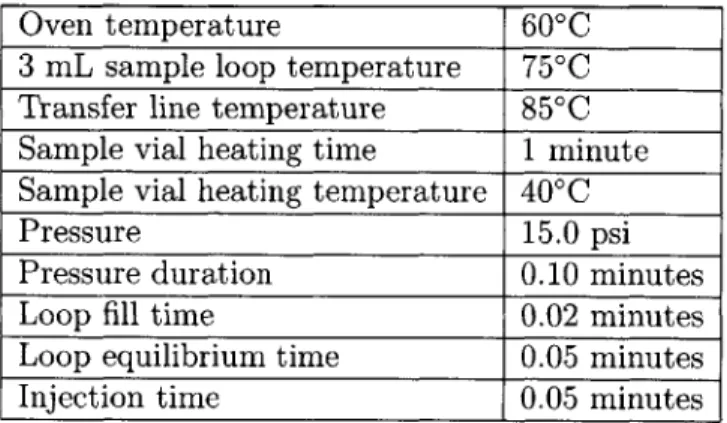
sampler through a transfer line into a silica column and carry it into to the FAIMS sensor. The sample carrier flow was regulated by the headspace sampler and was joined by a second flow of Nitrogen at 300 mL/min regulated by a mass flow controller5. The carrier gas and sample were ionized with 5 mCi of "Ni. Tables 1, 2, and 3 below show the parameters used for the headspace sampler, GC, and FAIMS sensor, respectively.

Oven temperature 600C

3 mL sample loop temperature 750C Transfer line temperature 850C Sample vial heating time 1 minute Sample vial heating temperature 40'C

Pressure 15.0 psi

Pressure duration 0.10 minutes

Loop fill time 0.02 minutes

Loop equilibrium time 0.05 minutes

Injection time 0.05 minutes

Table 1: Headspace sampler parameters

Inlet temperature 2500 C

Oven ramp initial hold time 0.5 minutes Oven ramp initial hold temperature 400C

Oven ramp rate 30'C/min

Final hold time 2 minutes

Final hold temperature 1700C Detector heating block temperature 140 C

Table 2: GC parameters

Emax 1200V/cm

V range [-35,5]V

Number of V samples 100

Sample duration 1.6 seconds Number of time samples 500

Table 3: FAIMS parameters

5

3.3

Detector Implementation

All statistical detectors were implemented in MATLAB, with the input being a single FAIMS signal, a matrix 500 x 100 in size. Each sample signal, denoted by r(t, V),

consisted of 500 scans in time, t, and 100 points in compensation voltage, V, yielding a matrix of ion intensities with 50,000 entries.

As noted previously, the FAIMS sensor outputs a pair of 3-dimensional signals cor-responding to the positive and negative ion quantities. However, the negative ion signal was not found to yield any difference among the means of various concentrations of chlorite and water for this particular application (data not shown). As a result, we focus our work on the positive ion signal, and all received signals, r(t, V), refer to the positive

ion FAIMS output signal.

As we empirically determined from various FAIMS spectral traces, there is an element of time variance that exists within the data; two data samples from the exact same solution will look slightly different if they were run at different times. As a result, it is difficult to acquire large quantities of consistent data, and we have chosen to focus all of our testing and training on the two runs of data comprising 76 total samples. Because of the limited number of samples, we have both trained and tested on the same data. Although this is a limitation of our analysis, we were able to establish proof-of-concept for applying statistical detection algorithms to this complex data type.

For the wavelet transforms, the MATLAB Wavelet Toolbox was used for the function 'wavedec' to implement the wavelet transforms on the data.

3.4

Data Description

As mentioned previously, each data sample signal, r(t, V), consists of 100 scans over

a compensation voltage range of [-35, 5] V, and 500 scans over a time range of [0, 800] seconds.

a particular class) of pure water and chlorite-contaminated water at 2.5 ppm and 40 ppm. Water and chlorite at 2.5 ppm are relatively visually indistinguishable, while the difference becomes much more obvious at 40 ppm of chlorite. A small peak arises in the 40 ppm chlorite mean while another peak disappears as compared to the 2.5ppm concentration of chlorite. Arrows indicate the areas in the data that are visually different between concentrations.

0.4

--

10 __0.3

> -20

0.2

-30

0.1

-30

Mean of Water

100

200

300

400

500

600

700

800

time (seconds)

0

0.4

--

10

0.3

>

-20

0.2

0.1

-30

_{Mean of Chlorite (2.5 ppm)}

100

200

300

400

500

600

700

800

time (seconds)

0

--

10

_0.3

>

-20

0.2

0.1

-30

_{Mean of CNorite (40 ppm)}

100

200

300

400

500

600

700

800

time (seconds)

Figure 5: Top-View Plots of FAIMS Spectra for Water and Chlorite-Contaminated Water at 2.5 ppm and 40 ppm

4

Problem Formulation and Development

4.1

Problem Description

We wish to develop a statistical detector to determine with the lowest possible rate of error whether or not chlorite is present in the water; the detector output is a binary decision and we wish to minimize the rate of missed detections and false alarms.

While the final output of the detector is binary, the unthresholded detector test statistic is a random variable indicative of how much of the input sample lies in the domain of the contaminated water and how much of the input sample falls in the domain of pure water. This random variable will have a different mean and variance for a given training concentration and a given testing concentration, but the goal is for the means to be as far apart as possible for pure water and contaminated water, and for the variance to be as small as possible. Thus, the distribution of this random variable serves as an important tool for a particular detector as the probability distribution function (PDF) and parameters under each hypothesis dictate how far apart the classes are under a given detection algorithm.

4.2

Bayesian Derivation

We have the null and test hypotheses, HO and H1, for each single observation, r;

given this, we wish to estimate which hypothesis occurred and minimize the probability of error associated with this estimate. Thus, for every received signal, r, we wish to devise a mapping f(r) between the received signal and the estimated hypothesis. The problem becomes, for each particular r, to determine which hypothesis minimizes the probability of error. The probability of error will be the probability that the actual event is different from the hypothesis we choose.

Pr[H = HIr = r]

Similarly, for any given received signal r, the probability of error associated with choosing H1 will be the probability that the actual hypothesis was HO, conditioned on

receiving r:

Pr[H = Hoir = r] ₍₁₀₎

Since we are attempting to minimize the probability of error, the optimal decision rule is to choose HO when the probability of error for choosing HO is smallest, or when:

Pr[H = Hojr = r] > Pr[H = H1jr = r] ₍₁₁₎

By using Bayes' Rule [8], we recall that:

Pr[H = Hmr = r] = PrIH (r IH,) Pm

PrIH(rIHO)P +PrIH(YIH1)P

where PO and P denote the a priori probabilities of hypotheses HO and H1, respectively.

By plugging this into the expression for the optimal decision rule in (11), we see that we should choose HO when:

PrIH(rIHO)PO > PrIH(rHl)P

or, equivalently, when:

pr|H(rIHo) P1

Pr|H(r|H1) Po

(13)

(14) If we further assume that PrIH(rHo) and PrjH(r|H1) are Gaussian distributions (which will be the case when the variation on the received signal is due entirely to Gaussian (12)

noise, as we will discuss in the next section), then we can simplify this expression for the decision rule further. Here we denote mo as E[rIHo], mi as E[rIH], EO as E[(r

-mo)(r -mo)TIHo], and E1 as E[(r -mi)(r -mi)

T

H], where E[.] indicates the expected value of the given random variable. This yields the following decision rule to choose HO when:

1 e-(r-mo)TE-(r-mo)

1 e-(r-mi)T (rm1) (15)

V(27r)nlFe 2

P

where n is the dimension of the received signal. By simplifying, we obtain:

1 mo)TE-1 (r - mo) +

-(r

In

2 (- o 02

_PO

This general form of the likelihood ratio test yields two problems. This first is that we cannot determine with great accuracy the covariance matrix of either the null or test hypothesis, HO and H1. There are 500 x 100 = 50,000 total points in each received

signal, r(t, V), and therefore the covariance matrix we wish to estimate would be 50,000 x 50,000 in dimension. As discussed in [7], if we wish to estimate this covariance matrix, we would require at least 50,000 distinct data samples for each of the hypotheses, HO and H1. To maintain an average loss ratio of better than one-half, we would require

at least 2 x 500 x 100 = 100,000 samples of each case (with and without chlorite) to sufficiently calculate the covariance [7]. Given our limited number of data samples, this is not feasible.

The other issue that arises is that even if we were to have the appropriate covariance matrix estimates, to invert such a large matrix would require substantial computing power. While such a feat can be accomplished on a standard personal computer, to implement on a microcontroller or FPGA, the most cost-effective portable computation

be feasible to implement in a cost-effective portable water monitoring tool.

These issues lead to a need of a reduction in dimensionality or a simplified covariance matrix. If we can find a way to represent the relevant information in the signal with only a few coefficients, then we will have enough data samples to form a valid estimate of the covariance matrix of those coefficients and consequently perform detection on a small number of coefficients. Alternatively, we can make simplifications and assumptions about the covariance matrix of the original data sample. If we can support the notion that the covariance matrix is diagonal (i.e., a constant variance multiplied by the identity matrix), then the inversion of the covariance matrices requires only a division of the constant variance (since the inverse of the identity matrix is itself). By using these simplifications, we can perform detection on the original 50,000 points in each data signal.

5

Noise Analysis

In order to properly characterize the received signal, r(t, V), we need to analyze the

noise and variation on the signal. Specifically, we seek to gain an understanding of Eo and El, the covariances of the signal under hypotheses Ho and H1. The covariance is an

indication of how correlated different random variables are; if the covariance is diagonal, then the random variables are completely uncorrelated. If the covariance is not diagonal, then the different random variables are not independent, but are instead influenced and affected by one another. As derived previously, E0 and El are necessary for use in the

optimal detector, and thus we would like to make a valid estimate. Toward this end, we are looking to characterize the covariance with time, t, and the covariance with voltage,

V, for the purpose of gaining information about the interdependence of points within

the received signal r(t, V).

5.1

Overview of Analysis and Estimation

As mentioned earlier, we assume that all variation on the signal comes from the additive random noise and is independent of the water background or chlorite signal. As a result, we can begin a preliminary characterization of the noise by generating a histogram of the points produced by the FAIMS sensor that occur before the sample has been injected into the FAIMS setup. During this time, the carrier gas is flowing through the FAIMS setup and the sensor is measuring the ion intensity variation, but there is no water background or chlorite signal.

The choice to use the points before the sample has been introduced (and thus evident at the sensor output) comes from the need to analyze inherent sensor variation without the presence of any signal, either from water or chlorite. The introduction of the signal would distort the underlying distribution of the noise, preventing us from adequately

data points instead of requiring a histogram for each of the 50,000 data points in the sample.

In addition to the distribution of the individual noise points, we are interested in their interdependency upon one another. In order to estimate an accurate covariance matrix of size 50,000 x 50,000 entries, it would be necessary to have more than 100,000 samples, which is impractical. At a rate of approximately 11 minutes per sample, 100,000 samples would require a constant data acquisition of more than two years. As a compromise, we can accept the lack of of a full covariance estimate and instead make an approximation through the covariance in time and the covariance in voltage. These estimates are discussed below.

5.2

Covariance in Time

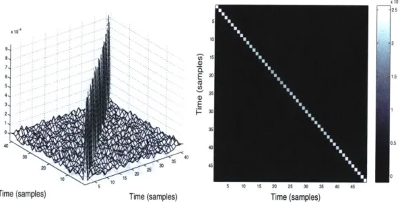
In order to address the issue of dependency between noise samples, it is necessary to estimate a covariance of the noise. Unfortunately, it is unrealistic to estimate a 50,000 x 50,000 sample matrix with such a small number of datasets. Thus, we are focusing first on the covariance with respect to time, and then on the covariance with respect to voltage. To estimate the covariance in time, the sample time for a given voltage scan was used to calculate the expected product as a function of time scan. A total of 76 different signals (r(t, V)) with each contributing 15 rows of V scans was used to estimate the

covariance. The covariance estimate, Et(i,

j)

Et(i, j) = E[(r(i, V*) - f(i, V*))(r(j, V*) - f(j, V*))] (17)

where V* indicates one of the first 15 V, points in the signal before any contaminant was introduced.

x 10, 8 X 10 10 - e, 7 5 5 4 -3 ---, 35 3 0 0 2 50 4 40 -- 50 50, 30 40 0, 10 0 5 10 15 20 25 30 35 40 45 50 55

Vc (samples) Vc (samples) Vc (samples)

Figure 6: Covariance in V (mesh view) Figure 7: Covariance in V, (top view)

5.3

Covariance in Vc

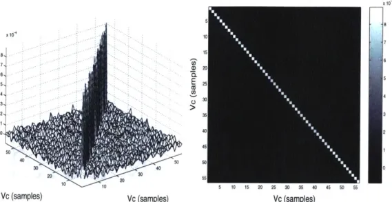
Similarly to the estimate of the covariance in time, it was necessary to estimate the covariance in compensation voltage. To estimate the covariance with respect to compensation voltage, the sample voltage lag for a given time scan was used to calculate the expected product as a function of compensation voltage. A total of 76 different signals (r(t, V)) with each contributing 15 rows of t scans was used to estimate the covariance. The covariance estimate, Ev (i,

j)

Ev, (i, j) = E[(r(t*, i) - f(t*, i))(r(t*, j) - f(t*, j))] (18)

where t* indicates one of the first 15 t points in the signal before any chlorite contaminant was introduced. Figures 6 and 7 show the estimated covariance matrix with respect to compensation voltage, while figures 8 and 9 show the estimated covariance matrix with respect to time.

X i0F, X104 6 E _1.5 0 (I2 15. 4, 25 10 ". 0. 5 5 10 15 20 25 30 35 40 45

Time (samples) Time (samples) _{Time (samples)}

Figure 8: Covariance in time (mesh view) Figure 9: Covariance in time (top view)

the diagonal entries are all approximately 9.27 x 10-4 (mv)2

for both covariances, with a variation of less than 5% between diagonal entries in the same covariance and between the two covariance matrices. This provides a very strong indication that the noise is uncorrelated both in time and in voltage, and further that variance is equal for all points. Given that the noise is uncorrelated in both dimensions, it is reasonable to assume that the noise will be uncorrelated for all coordinate points (t, V) in the measured data and thus that the overall covariance matrix will be white and diagonal as well. We will employ this key assumption, based on these experiments, in the implementation of statistical detectors.

5.4

Histograms

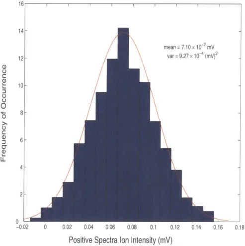
The histogram for all data points of the baseline sensor output is shown in Figure 10, along with a fitted Gaussian distribution with the mean and variance obtained from the data. As mentioned previously in Section 2.3, there is a level of quantization that makes it difficult to estimate with a high resolution the histogram of data points, and

thus the resolution shown is the highest attainable.

I I I I I I I I I

mean = 7.10 x 10-2 mV

var = 9.27 x 104 (mV)2

0 0.02 0.04 0.06 0.08 0.1 0.12

Positive Spectra Ion Intensity (mV)

0.14 0.16 0.18

Figure 10: Histogram of noise with fitted Gaussian probability distribution function

The Gaussian distribution shown in Figure 10, when combined with the indication of decorrelation as seen in the covariance estimates, allows us to make the assumption that the overall covariance matrix is white and that each of the noise points is independent and identically distributed. The mean, p, and variance, a2, of the noise was found to be 7.10 x 10-2 mV and 9.27 x 104 (mv)2 , respectively. 16 14 12 10 8 6 C 1-0 40

0

6

Matched Filter and ACE Detectors

6.1

Matched Filter

6.1.1 Overview

As mentioned previously, there are two statistical analysis routes which we have chosen to take. The first route is a simplifed assumption on the covariance estimate which allows us to utilize noise that is independent and identically distributed (IID) and therefore has a diagonal covariance matrix that is equal for both Ho and H1 and does

not require 100,000 samples to obtain a good estimate. Since we naively assume that the covariance matrix is white (i.e., the data is uncorrelated), the inversion is trivial and we can perform detection on the raw data. Thus, for a received signal, r(t, V), we use all of the 50,000 points of a given sample in the detection, but the detector algorithm assumes a simple covariance matrix. This assumption leads us to two detectors: matched filter and ACE (adaptive cosine estimate) which we investigate further.

The optimal binary detection test was derived in Section 3.2. Through the assump-tion that the covariance matrices for both Ho and H1 are the same and diagonal as

discussed above, we have E0 = El = a21 (where I denotes the identity matrix), and we

can simplify the decision rule to:

rT(m2 - i) > _{ln( i) + I (m'mo - mTmi)}

(19)

2 P 2g2 0

This leads to our definition of the matched filter raw detector output:

,L r T(Mo - Ml)

AMF(r) - r 2 (20)

output.

6.1.2 Assumptions

This detector makes the assumption that the noise is white and consequently that the covariance matrix of the noise is oa21, where a 2

denotes the variance. As mentioned previously, this assumption is supported in the previous section of noise analysis, but is not rigorously proven.

6.1.3 Implementation

The matched filter detector was trained separately on each of the five chlorite concen-trations: 2.5 ppm, 5 ppm, 10 ppm, 20 ppm, and 40 ppm. This detector was then tested on each of the data samples for pure water and the five concentrations of chlorite. The

likelihood ratio random variable is denoted by AMF (itrain, test), where [Lrain denotes

the training concentration and [test denotes the concentration of the received signal.

This random variable is characterized and documented with detector performance in section 7.2.

6.2

Adaptive Cosine Estimator

6.2.1 Overview

The adaptive cosine estimatator (ACE) [9] detector is similar to the matched filter detector, but relies on a measure of the angle between the received signal and the target signatures instead of a measure of the energy overlap. This is particularly important when there is a scaling factor of the received signal that varies with time or data collec-tion. Unlike with the matched filter detector, the ACE detector will maintain a constant false alarm rate (CFAR) even with scale variations in the received signal, which is an important property for a deployed sensor. While the matched filter detector examines

the inner product of the received signal and the difference of the means, the ACE de-tector examines the angle between the received signal and the difference of the means as shown below:

,L r T(MO - M1)

AACE(r) = m (21)

liril * limo - mill

where

IF-||

This value is then compared against a threshold for a binary detector decision.

6.2.2 Assumptions

This detector makes the assumption that the noise is white and consequently that the covariance matrix of the noise is a 2I. As mentioned previously, this assumption is

supported in the previous section of noise analysis.

6.2.3 Implementation

The ACE detector was trained separately on each of the five chlorite concentrations: 2.5 ppm, 5 ppm, 10 ppm, 20 ppm, and 40 ppm. This detector was tested on each of the data samples for pure water and the five chlorite concentrations. The likelihood ratio random variable is denoted by AACE(Ptest, Ptrain), where ptest denotes the testing

concentration and Ptrain denotes the training concentration. This random variable is characterized and documented with detector performance in section 7.2.

6.3

Performance Metrics

In order to evaluate different detectors, it is necessary to determine a set of met-rics with which to compare relative performance. The likelihood ratio output, AACE and AMF, for the ACE and MF detectors respectively, serves as an indicator of how

is necessary to calculate the means of A for each contaminant concentration and detec-tor. However, the mean itself does not indicate the degree of separation; the variance

must also be used. We denote Atrain and test as the training concentration and testing

concentration, respectively. We define the following measures: mdetector(Ptrain, Ptest) to denote the mean of Adetector

(Ptrain,

We propose a metric to define the level of separation between two classes:

'Ydetector (ttrain, Itest) =m-m- (22)

where mw and a, indicate the mean and standard deviation of A for the pure water class of a single type of detector and m, and oc indicate the mean and standard deviation of

A for the testing concentration, pt_est.

This quantity, -y, serves as a measure of detector performance evaluation that is independent of scaling factors of A and only depends on relative separation of the dis-tributions between two classes. To illustrate this point, consider the case of multiplying a particular detector output random variable by a constant a. If the previous means were given by me and mw, the new means will be a * m, and a * m,. Similarly, if the previous standard deviations were given by oc and a,, the new standard deviations will be au, and aox,. Consequently, the new 7 will be given by:

amc

-

amw

(23)

All factors of a cancel out, leaving the previous -y as before. This is important because

it demonstrates that -y gives an accurate measure of how separated two classes are and does so without regard to the absolute values of A.

We recognize that m and a completely characterize the distributions of the matched filter output, which is Gaussian. ACE, however, produces a T-distributed statistic which

is parameterized by a number of degrees of freedom and a non-centrality parameter [9]. However, we will focus on the first and second moments by utilizing our metric, 'y, to compare the relative separation power of the detectors.

6.4

Results

As discussed in the previous section, it is important to examine the statistics for the likelihood ratio test, AACE and AMF, to properly evaluate detector performance. Shown

below in Figures 11 and 12 are the median, lower quartile, upper quartile, range of data and outliers [38] for AACE and AMF respectively for each of the different classes (water

and chlorite at 5 different concentrations). In both cases, the detectors were trained on the lowest concentration of 2.5 ppm of chlorite. As can be seen, by choosing a threshold of -40 for the ACE detector or -1.2 for the matched filter detector, the classes could correctly be separated for all of the data, thus yielding perfect detection on the limited available data.

In order to more easily compare the two detectors, we calculate -y as a function of the testing concentration for the training concentration of 2.5ppm; the plot of -y for both the matched filter and ACE detector is shown below in Figure 13.

As can be seen from the comparative y values, the ACE detector performs better than the matched filter detector for all testing concentrations when trained at 2.5 ppm. Since the difference between the matched filter and ACE detectors lies in the measure of signal magnitude versus signal angle, it is evident that the received signal angle is a better indication of its class. This may be due to the fact that the data is scaled by an unknown and random factor which affects the relative energy in the signal. We can conclude that the target signature is best characterized by the angle it maintains instead of the energy and magnitude of relative points within the signal.

-15 + _median - upper/lower quartile -data range -20- + outliers -25 E + -30 --0. C" 0 -35 -40 -45- -50-I I I I I I Pure Water 2.5 ppm 5 ppm 10 ppm 20 ppm 40 ppm Chlorite Chlorite Chlorite Chlorite Chlorite Figure 11: ACE detector output (AACE) statistics (itrain=2-5 ppm)

centrations are not simply stronger versions than those at lower concentrations. This motivates the need for more sophisticated techniques to analyze the target signals.

In Figures 14 and 15, -y is plotted for the ACE and Matched Filter Detectors, re-spectively, for all training and testing concentrations. As can be seen, 7 is uniformly higher when the testing concentration matches the training concentration (i.e., when the signature the detector is looking for is the one it was trained on). This makes intuitive sense, as the detector performance should be higher when the testing concentration is the same as the training concentration. However, we might have expected -IMF to be increasing with the testing concentration if the chlorite signal were increasing in magni-tude with concentration. Since this is not the case, we can infer that the chlorite signal

-0.4 + median -upper/lower quartile -data range + outliers

H

Chlorite Chlorite Chlorte

Figure 12: Matched filter detector output (AMF) Statistics (pZtrain=2.5 ppm)

varies nonlinearly. This gives another motivating factor for the need to analyze the tar-get signals of various concentrations not simply as an increase in signal, but perhaps as a subspace inhabited by the class of chlorite-contaminated signals.

C-LO) C11 IL 40 ppm Chlorite

25 Matched Filter SACE 20- 15-10

I

I

.5 ppm) E.

LO

40 0 V train -5PPM 35~ M 9train=1 ppm

IZ

0

40

U

E

7 Multidimensional Target Subspaces

7.1

Overview & Motivation

The matched filter and ACE detectors discussed in previous sections assume that the target signatures (means) of various chlorite concentrations are scaled versions of one another. The detectors treat the training concentration mean as a vector and look for the received signal to be in the same direction as that vector, and expect that if the received signal concentration is higher, the received signal magnitude will increase, but the direction will be the same.

However, we have empirical evidence to show that the signatures of various concen-trations of chlorite-contaminated water do not behave as discussed above. In Figures 16 and 17, we have plotted the mean energy as a function of concentration and the mean angle between higher concentrations of chlorite and chlorite at 2.5 ppm.

2.5 ppm 5 ppm 10 ppm 20 ppm

Chlorite Concentration

40 ppm

Figure 16: Mean energy for chlorite

'0 0) a C 10 5 ppm 10 ppm 20 ppm Chlorite Concentration

Figure 17: Angle between concentrations

As can be seen, the energy does not increase with concentration, as we would expect

35 30 C w 20 15

t

the signature of another concentration and chlorite at 2.5 ppm is significant and becomes more so as the concentration increases. It is evident that the signature is not simply scaling with concentration. Instead, higher concentrations of chlorite-contaminated wa-ter develop new features in varying locations, (t, V), and, in reference to the vector analogy, vary their direction as the concentration increases.

In a practical implementation of this detector, we will be looking to monitor a given water source and sound an alarm the first time chlorite is detected in the water. However, using this method, we are unable to predict at what concentration level the contami-nant will first appear, making it difficult to best train the detector on the appropriate concentration.

In an effort to address this point and create a set of detectors that are more robust to varying levels of chlorite, we aim to create a subspace that is spanned by multiple levels of chlorite. As we recall from the single dimensional matched filter and ACE detectors, we projected the received signal onto the difference between the mean of chlorite and the mean of water. This quantity served as a measure of the energy and made up the basis for the matched filter detector. When this quantity was normalized by the energy in the signal, it became a measure of the angle of the signal and served as the basis for the ACE detector.

In the multidimensional case, we wish to extend the dimension of the target sub-space onto which we project the received signal. Instead of consisting of a single vector composed of the mean difference of water and a single concentration of chlorite, we will create a subspace spanned by multiple vectors composed of the difference of water and varying concentrations of chlorite. The amount of energy in the received signal that lies in this subspace will be the basis for the matched filter multidimensional subspace detector. The angle that the received signal makes with this subspace will be the basis for the ACE multidimensional subspace detector.

received signal lies in, we also open up the possibility of including more of the subspace that is spanned by pure water. This inclusion of multiple subspaces will increase the amount of the received signal that lies in those multiple subspaces, but will do so for both chlorite-contaminated water and pure water. Thus, a multidimensional subspace detector might perform better than a single dimensional detector compared to testing on a concentration different than that it was trained on, but we do not necessarily expect it to perform as well as the single dimensional detector when testing on the same concentration it was trained on.

For this section, we continue to maintain the previous assumption that the covariance is white and the noise is uncorrelated in both time and compensation voltage.

7.2

Implementation

We define a projection matrix, PD, whose subspace, 4, is spanned by the differences of the mean of water and means of the the five chlorite concentration signatures, denoted

here by mdl, mc2, m3, md4, and md5, where each is a column vector of length 50,000.

The water mean is denoted by m,. The subspace, 1 is given by:

I

I

I

(mdi - mw) (mcl2 - m.) (md3 - m.) (md4 - m.) (mcl5 - m)

I

I

I

The orthogonal projection matrix, PD, which projects a received signal onto the subspace is given by [16]:

p"I

(24)

Thus, the corresponding matched filter detector measures the energy of the received signal in the subspace, given by rTP r. The ACE detector measures the cosine-squared