Mobile and remote inertial sensing with atom interferometers

HAL Id: hal-00908849

https://hal.archives-ouvertes.fr/hal-00908849v2

Submitted on 28 May 2014

HAL is a multi-disciplinary open access

archive for the deposit and dissemination of

sci-entific research documents, whether they are

pub-lished or not. The documents may come from

teaching and research institutions in France or

abroad, or from public or private research centers.

L’archive ouverte pluridisciplinaire HAL, est

destinée au dépôt et à la diffusion de documents

scientifiques de niveau recherche, publiés ou non,

émanant des établissements d’enseignement et de

recherche français ou étrangers, des laboratoires

publics ou privés.

Mobile and remote inertial sensing with atom

interferometers

Brynle Barrett, Pierre-Alain Gominet, Etienne Cantin, Laura

Antoni-Micollier, Andrea Bertoldi, Baptiste Battelier, Philippe Bouyer, Jean

Lautier, Arnaud Landragin

To cite this version:

Brynle Barrett, Pierre-Alain Gominet, Etienne Cantin, Laura Antoni-Micollier, Andrea Bertoldi, et

al.. Mobile and remote inertial sensing with atom interferometers. International School of Physics

”Enrico Fermi” on Atom Interferometry, Jul 2013, Varenna, Italy. �hal-00908849v2�

B. Barrett, P.-A. Gominet, E. Cantin, L. Antoni-Micollier, A. Bertoldi, B. Battelier and P. Bouyer

Laboratoire Photonique Num´erique et Nanosciences, Institut d’Optique d’Aquitaine and Univer-sit´e de Bordeaux, rue Fran¸cois Mitterrand, 33400 Talence, France

J. Lautier, and A. Landragin

LNE-SYRTE, Observatoire de Paris, CNRS and UPMC, 61 avenue de l’Observatoire, F-75014 Paris, France

Summary.— The past three decades have shown dramatic progress in the ability to manipulate and coherently control the motion of atoms. This exquisite control offers the prospect of a new generation of inertial sensors with unprecedented sen-sitivity and accuracy, which will be important for both fundamental and applied science. In this article, we review some of our recent results regarding the applica-tion of atom interferometry to inertial measurements using compact, mobile sensors. This includes some of the first interferometer measurements with cold39K atoms, which is a major step toward achieving a transportable, dual-species interferometer with rubidium and potassium for equivalence principle tests. We also discuss fu-ture applications of this technology, such as remote sensing of geophysical effects, gravitational wave detection, and precise tests of the weak equivalence principle in Space.

c

1. – Introduction

In 1923, Louis de Broglie generalized the wave-particle duality of photons to material particles [1] with his famous expression, λdB= h/p, relating the momentum of the

parti-cle, p, to its wavelength. Shortly afterwards, the first matter-wave diffraction experiments were carried out with electrons [2], and later with a beam of He atoms [3]. Although these experiments were instrumental to the field of matter-wave interference, they also revealed two major challenges. First, due to the relatively high temperature of most accessible particles, typical de Broglie wavelengths were much less than a nanometer (thousands of times smaller than that of visible light)—making the wave-like behavior of particles difficult to observe. For a long time, only low-mass particles such as neutrons or electrons could be coaxed to behave like waves since their small mass resulted in a relatively large de Broglie wavelength. Second, there is no natural mirror or beam-splitter for matter waves because solid matter usually scatters or absorbs atoms. Initially, diffraction from the surface of solids, and later from micro-fabricated gratings, was used as the first type of atom optic. After the development of the laser in the 1960’s, it became possible to use the electric dipole interaction with near-resonance light to diffract atoms from “light gratings”.

In parallel, the coherent manipulation of internal atomic states with resonant radio frequency (rf) waves was demonstrated in experiments by Rabi [4]. Later, pioneering work by Ramsey [5] lead to long-lived coherent superpositions of quantum states. The techniques developed by Ramsey would later be used to develop the first atomic clocks, which were the first matter-wave sensors to find industrial applications.

From the late 1970’s until the mid-90’s, a particular focus was placed on laser-cooling and trapping neutral atoms [6, 7, 8, 9, 10] which eventually led to two nobel prizes in physics [11, 12]. Heavy neutral atoms such as sodium and cesium were slowed to velocities of a few millimeters per second (corresponding to temperatures of a few hundred nano-Kelvin), thus making it possible to directly observe the wave-like nature of matter.

The concept of an atom interferometer was initially patented in 1973 by Altschuler and Franz [13]. By the late 1980s, multiple proposals had emerged regarding the ex-perimental realization of different types of atom interferometers [14, 15, 16, 17]. The first demonstration of cold-atom-based interferometers using stimulated Raman transi-tions was carried out by Chu and co-workers [18, 19, 20]. Since then, the field of atom interferometry has evolved quickly. Although the state-labeled, Raman-transition-based interferometer remains the most developed and commonly used type, a significant effort has been directed toward the exploration and development of new types of interferometers [21, 22, 23, 24, 25, 26, 27, 28, 29, 30, 31, 32, 33, 34, 35, 36, 37].(1₎

Atom interferometry is nowadays one of the most promising candidates for ultra-precise and ultra-accurate measurements of inertial forces and fundamental constants

(1_{) For a more complete history and review of atom interferometry experiments see, for example,}

[39, 40, 41, 42, 43]. The realization of a Bose-Einstein condensation (BEC) from a dilute gas of trapped atoms [9, 10] has produced the matter-wave analog of a laser in optics [44, 45, 46, 47]. Similar to the revolution brought about by lasers in optical interferometry, BEC-based interferometry is expected to bring the field to an unprecedented level of accuracy [48].

Lastly, there remained a very promising application for the future: atomic inertial sensors. Such devices are inherently sensitive to, for example, the acceleration due to gravity, or the acceleration or rotation undergone by the interferometer when placed in a non-inertial reference frame. Apart from industrial applications, which include navigation and mineral prospecting, their ability to detect minuscule changes in inertial fields can be utilized for testing fundamental physics, such as the detection of gravitational waves or geophysical effects. Inertial sensors based on ultra-cold atoms are only expected to reach their full potential in space-based applications, where a micro-gravity environment will allow the interrogation time, and therefore the sensitivity, to increase by orders of magnitude compared to ground-based sensors.

The remainder of the article is organized as follows. In sect. 2, we review, briefly, the basic principles of an interferometer based on matter waves and give some theoretical background for calculating interferometer phase shifts. Section 3 provides a detailed description of the interferometer sensitivity function, and the important role it plays in measuring phase shifts in the presence of noise. In sect. 4, we discuss various types of lab-based inertial sensors. This is followed by sect. 5 with a description of mobile sensors and recent experimental results. Section 6 reviews some applications of remote atomic sensors to geophysics and gravitational wave detection. Finally, in sect. 7, we outline the advantages of space-based atom interferometry experiments, and describe two proposals for precise tests of the weak equivalence principle. We conclude the article in sect. 8. 2. – Theoretical background

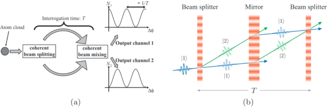
2.1. Principles of a matter-wave interferometer . – Generally, atom interferometry is performed by applying a sequence of coherent beam-splitting processes separated by an interrogation time T , to an ensemble of particles. This is followed by detection of the particles in each of the two output channels, as is illustrated in fig. 1(a). The interpreta-tion in terms of matter waves follows from the analogy with optical interferometry. The incoming matter wave is separated into two different paths by the first beam-splitter, and the accumulation of phase along the two paths leads to interference at the last beam-splitter. This produces complementary probability amplitudes in the two channels, where the detection probability oscillates sinusoidally as a function of the total phase difference, ∆φ. In general, the sensitivity of the interferometer is proportional to the enclosed area between the two interfering pathways.

A well-known configuration of an atom interferometer is designed after the optical Mach-Zehnder interferometer: two splitting processes with a mirror placed at the center to close the two paths [see fig. 1(b)]. Usually, a matter-wave diffraction process replaces the mirrors and the beam-splitters and, when compared with optical diffraction, these

(a)

Beam splitter Mirror Beam splitter

(b)

Fig. 1. – (Colour online) (a) Principle of an atom interferometer. An initial atomic wavepacket is split into two parts by a coherent beam-splitting process. The wavepackets then propagate freely along the two different paths for an interrogation time T , during which the two wavepackets can accumulate different phases. After this time, the wavepackets are coherently mixed and interference causes the number of atoms at each output port, N1and N2, to oscillate sinusoidally

with respect to this phase difference, ∆φ. (b) The basic Mach-Zehnder configuration of an atom interferometer. An atom initially in a quantum state |1⟩ is coherently split into a superposition of states |1⟩ and |2⟩. A mirror is placed at the center to close the two atomic trajectories. Interference between the two paths occurs at the second beam-splitter.

processes can be separated either in space or in time. During the interferometer sequence, the atom resides in two different internal states while following the spatially-separated paths. In comparison, interferometers using diffraction gratings (which can be comprised of either light or matter) utilize atoms that have been separated spatially, but reside in the same internal state. This is the case, for example, with single-state Talbot-Lau interferometers [21, 24, 34, 33], which have also been demonstrated with heavy molecules [27].

Light-pulse interferometers work on the principle that, when an atom absorbs or emits a photon, momentum must be conserved between the atom and the light field. Consequently, when an atom absorbs (emits) a photon of momentum !k, it will receive a momentum impulse of !k (−!k). When a resonant traveling wave is used to excite the atom, the internal state of the atom becomes correlated with its momentum: an atom in its ground state |1⟩ with momentum p (labeled |1, p⟩) is coupled to an excited state |2⟩ of momentum p + !k (labeled |2, p + !k⟩).

The most developed type of light-pulse atom interferometer is that which utilizes two-photon velocity-selective Raman transitions to manipulate the atom between separate long-lived ground states. With the Raman method, two laser beams of frequency ω1 and

ω2are tuned to be nearly resonant with an optical transition. Their frequency difference

ω1− ω2 is chosen to be resonant with a microwave transition between two hyperfine

ground states. Under appropriate conditions, the atomic population oscillates between these two states as a function of the interaction time with the lasers, τ . The “Rabi” frequency associated with this oscillation, Ωeff, is proportional to the product of the two

the optical detuning from a common hyperfine excited state. Thus, pulses of the Raman lasers can be tuned to coherently split (with a pulse area Ωeffτ= π/2) or reflect (with a

pulse area Ωeffτ = π) the atomic wavepackets.

When the Raman beams are counter-propagating (i.e. when the wave vector k2 ≈

−k1), a momentum exchange of approximately twice the single photon momentum

ac-companies these transitions: !(k1− k2) ≈ 2!k1. This results in a strong sensitivity to

the Doppler frequency associated with the motion of the atom.(2₎

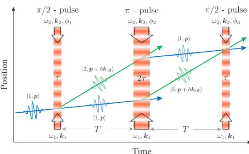
Henceforth, we shall consider only the most commonly used interferometer config-uration, which is the so-called “three-pulse” or “Mach-Zehnder” configuration formed from a π/2 − π − π/2 pulse sequence to coherently divide, reflect and finally recom-bine atomic wavepackets.(3_{) This pulse sequence is illustrated in fig. 2. Here, the first}

π_{/2-pulse excites an atom initially in the |1, p⟩ state into a coherent superposition of} ground states |1, p⟩ and |2, p + !keff⟩, where keff is the difference between the two

Ra-man wave vectors. In a time T , the two parts of the wavepacket drift apart by a distance !k_effT /M . Each partial wavepacket is redirected by a π-pulse which induces the tran-sitions |1, p⟩ → |2, p + !k⟩ and |2, p + !keff⟩ → |1, p⟩. After another interval T the two

partial wavepackets overlap again. A final π/2-pulse causes the two wavepackets to re-combine and interfere. The interference is detected, for example, by measuring the total number of atoms in the internal state |2⟩ at any point after the Raman pulse sequence. This allows one to easily access the interferometer transition probability, which oscillates sinusoidally with the interferometer phase Φ:

(1) P (Φ) = N1

N1+ N2 = P0−

C

2 cos(Φ).

Here, N1(N2) represents the number of atoms detected in the state |1⟩ (|2⟩), the offset

of the probability is usually P0 ∼ 0.5, and C is the contrast of the fringe pattern. In

comparison, the detection scheme for single-state interferometers [22, 21, 24, 33, 34, 35, 49] requires a near-resonant traveling wave laser to coherently backscatter off of the atomic density grating formed at t = 2T . Here, the interferometer phase can be detected by heterodyning the backscattered beam with an optical local oscillator.

Another positive feature of this type of interferometer is that the linewidth of stim-ulated Raman transitions can be adjusted to tune the spread of transverse velocities addressed by the pulse. This relaxes the “velocity collimation” requirements and can increase the number of atoms that contribute to the interferometer signal. In contrast, Bragg scattering from standing waves is efficient only for narrow velocity spreads, where the width is much less than the photon recoil velocity.

(2_{) In contrast, when the beams are aligned to be co-propagating (i.e. k}

2 ≈ k1), these

transi-tions have a negligible effect on the atomic momentum and the transition frequency is essentially insensitive to the Doppler shift of moving atoms.

(3) Other possible configurations include that of the Ramsey-Bord´e interferometer: π/2−π/2− π/2 − π/2, or those utilizing Bloch-oscillation pulses or large momentum transfer pulses to increase the interferometer sensitivity.

Time

Position

Fig. 2. – (Colour online) Three-pulse atom interferometer based on stimulated Raman transi-tions. Here, keff = k1+ k2 is the effective wave vector for the two-photon transition, and the

pulse duration τ is defined by Ωeffτ = π/2.

2.2. Phase shifts from the classical action. – In this section, we give a brief review of the Feynman path integral approach to computing the interferometer phase shift from the classical action. Then, in sect. 2.3, we apply this formalism to the specific example of the three-pulse interferometer in the presence of a constant acceleration. Both of these sections are largely based on ref. [50].

According to the principle of least action, the actual path, z(t), taken by a classical particle is the one for which the action S is extremal. The action is defined as

(2) S =

! tb

ta

dtL[z(t), ˙z(t)],

where L(z, ˙z) is the Lagrangian of the system. The action corresponding to this path is called the classical action, Scl, and it can be shown to depend on only the initial and

final points {zata, zbtb} in spacetime: Scl(zbtb, zata).

Given the initial state of a quantum system at time ta, the state at a later time tb is

determined through the evolution operator U

(3) |Ψ(tb)⟩ = U(tb, ta) |Ψ(ta)⟩ .

The projection of this state on the position basis gives the wavefunction at time tb

(4) Ψ(zb, tb) =

!

dzaK(zbtb, zata)Ψ(za, ta),

where K is called the quantum propagator, and is defined as [50] (5) K(zbtb, zata) ≡ ⟨zb| U (tb, ta) |za⟩ .

The quantity |K(zbtb, zata)| gives the probability of finding the particle at the spacetime

position zbtb, provided it started from the point zata. As demonstrated by Feynman [51],

the quantum propagator can be expressed equivalently as a sum over all possible paths, P, connecting point zata to zbtb. (6) K(zbtb, zata) ∝ " P eiSP/!₌ ! b a dz(t)eiSP/!_.

Since the action is extremal for the classical path, the phase factors eiSP/! _associated

with neighboring paths tend to interfere constructively. For other paths, SP generally

varies rapidly compared to Scl, thus, they interfere destructively and don’t contribute to

K(zbtb, zata).

In the general case of a system that can be described by a Lagrangian that is, at most, quadratic in z(t) and ˙z(t), the quantum propagator can be expressed in the simple form [50]

(7) K(zbtb, zata) = F (tb, ta)eiScl(zbtb,zata)/!,

where F (tb, ta) is a function that depends on only the initial and final times. Inserting

this result into eq. (4) for the final wavefunction gives (8) Ψ(zb, tb) = F (tb, ta)

!

dzaeiScl(zbtb,zata)/!Ψ(za, ta).

In the integral over za, the neighborhood of the positions where the phase of eiScl(zbtb,za,ta)/!

cancels the phase of φ(za, ta) will be the most dominant. Equation (8) has a simple

inter-pretation: the phase of the final wavefunction, ϕb, is determined by the classical action,

Scl(zbtb, zata), and the phase of the wavefunction at the initial point, ϕa. In the case of

an atom interferometer, the phase shift introduced between two arms is then simply the difference in classical action between the two closed paths.

2.3. Application to the three-pulse interferometer . – In this section, we will apply the formalism of the previous section to compute the phase shift of the three-pulse Mach-Zehnder atom interferometer (shown in fig. 2) in the presence of the acceleration due to gravity, g. This type of interferometer, which has the Raman lasers oriented along the vertical direction, was first demonstrated by Kasevich & Chu [18, 19] and later developed for precise measurements of g in an atomic fountain [52, 39].

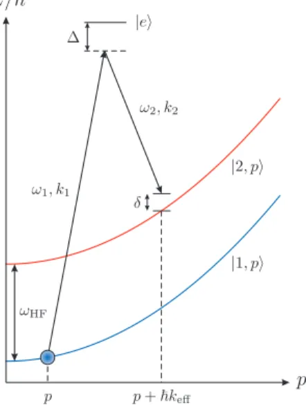
To evaluate the phase of the wavefunction after the interferometer pulse sequence (which governs the probability of detecting the atoms in either of the two ground states), we first describe the physics of two-photon Raman transitions. Figure 3 illustrates the energy levels of the atom as a function of momentum, p. Two counter-propagating plane waves, with frequencies ω1 and ω2, wave vectors k1 and k2, and phase difference φ,

induce a transition between ground states |1⟩ and |2⟩ via off-resonant coupling from a common excited state |e⟩. In the process, the atom scatters one photon from each beam

Fig. 3. – (Colour online) Raman transition energy levels. Atoms initially in the state |1, p⟩ are transferred to |2, p + !keff⟩ via a two-photon transition from counter-propagating Raman beams.

The hyperfine ground states are separated by !ωHF in energy, the one-photon detuning of the

Raman beams from the common excited state |e⟩ is ∆, and δ is the two-photon detuning given by eq. (9).

for a total momentum transfer of !k_eff = !(k1+ k2). The two-photon detuning δ, which

characterizes the resonance condition for the Raman transition, is given by

(9) δ= ωeff − ωHF− k_eff · p M − !_k2 eff 2M ,

where ω_eff ≡ ω1 − ω2 is the frequency difference between Raman lasers, ωHF is the

hyperfine splitting between the two ground states, and M is the mass of the atom. (4₎

The last two terms in eq. (9) are the Doppler frequency and two-photon recoil frequency, respectively.

Under certain conditions, the Schr¨odinger equation associated with the interaction with the Raman beams can be written as

(10) d dt|Ψ(t)⟩ = d dt # c1(t) c2(t) $ = i #

|χ_eff| χ_effei(δt+φ)

χ∗

effe−i(δt+φ) |χeff|

$ # c1(t0)

c2(t0)

$ .

Here, the wave function is defined as a time-dependent superposition between the two

states:

(11) |Ψ(t)⟩ ≡ c1(t)e−i(p

2

/2M!)t

|1, p⟩ + c2(t)e−i[(p+!keff)

2

/2M!+ωHF]t

|2, p + !k_eff⟩ , and χeff ≡ Ωeff/2 = Ω∗1Ω2/∆ is half of the effective Rabi frequency. To arrive at eq. (10),

we have made a number of assumptions. First, the two Raman frequencies, ω1 and ω2,

are shifted far from the excited state such that their one-photon detuning is much larger than the transition linewidth: |∆| ) Γ. This allows us to ignore spontaneous emission effects and to eliminate the evolution of the excited state. Second, we assume the light intensity is constant, and that the two Rabi frequencies, Ω1and Ω2, associated with each

single-photon transition are equal: Ω1= Ω2 ≡ Ω. Third, we assume that |δ| * |Ω| and

ignore terms of order δ/Ω.

The solution to eq. (10) can be shown to be [53] (12) # c1(t) c2(t) $ = Uχ, φ(t, t0) # c1(t0) c2(t0) $ , where Uχ, φ(t, t0) is the evolution matrix from time t0→ t given by

(13) Uχ, φ(t, t0) = eiχeff(t−t0)

#

cos χeff(t − t0) iei(δt0+φ)sin χeff(t − t0)

ie−i(δt0+φ)_{sin χ}

eff(t − t0) cos χeff(t − t0)

$ . This expression describes the time-dependence of the atomic state amplitudes during a Raman pulse with phase difference φ and effective Rabi frequency Ωeff = 2χeff.

The total phase shift of the interferometer is equal to the difference in phase accu-mulated between the upper and lower pathways shown in fig. 4. It can be divided into three terms:

(14) Φtotal= Φpropagation+ Φlight+ Φseparation,

the phase shift from the free propagation of the atom, Φpropagation, the phase shift from

the atom-laser interaction during the Raman transitions, Φlight, and the phase shift

orig-inating from a difference in initial position of the interfering wave packets, Φseparation.

This last term is zero in this case, because the two wave packets are initially overlapped. However, it is non-zero when considering higher-order potentials [39], such as that pro-duced by a gravity gradient (which varies as z2_).

First, we examine the phase due to the propagation of the atoms along the two arms of the interferometer. To do this, we use the relation

(15) Φpropagation= (SL− SU)/!,

where SU and SL are the classical actions evaluated along the upper and lower atomic

Fig. 4. – (Colour online) Center-of-mass trajectories taken by the atoms in a Mach-Zehnder interferometer with gravity (dashed lines) and without gravity (solid lines).

Earth’s gravitational field, the classical action takes the form [50]

Scl(zbtb, zata) = ! tb ta dt% 1 2M v(t) 2 − Mgz(t) & =M 2 (zb− za)2 (tb− ta) − M g 2 (zb+ za)(tb− ta) − M g2 24 (tb− ta) 3_. (16)

Computing the difference in action between the two classical paths we find

(17) SL− SU= M

T (zD− zC)(zC+ zD− zA− zB− gT

2_).

However, from the equations of motion, it is straightforward to show that the vertices along the parabolic trajectories are related to the corresponding points along the straight-line paths in the absence of gravity (see fig. 4):

zA= zA0, zC= zC0− 1 2gT 2_{, z} D= zD0− 1 2gT 2_{, z} B= zB0− 2gT 2_.

Evaluating the last term in eq. (17), we find

(18) zC+ zD− zA− zB− gT2= zC0+ zD0− zA0− zB0 = 0,

since the straight-line trajectories enclose a parallelogram. Hence, the phase shift due to the propagation of the wavefunction vanishes: Φpropagation = 0. The interferometer

phase is then completely determined by the contribution from the interaction with the Raman beams, Φlight, which we now discuss.(5)

Similar to Φpropagation, the laser phase can be written as the difference between the

phase accumulated along the upper and lower pathways:

(19) Φlight= ϕlight_L − ϕlight_U .

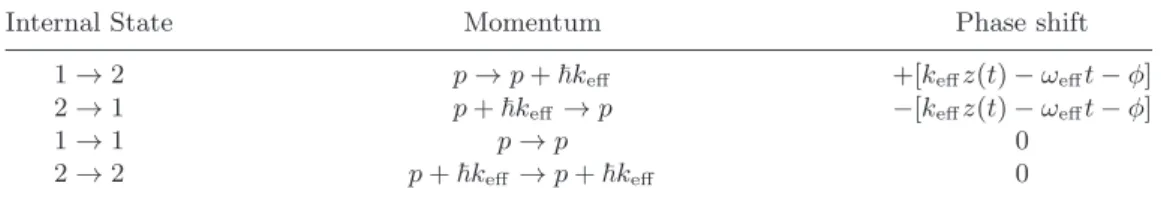
Table I summarizes the laser phase contributions to the wave function that result from Raman transitions [39]. As a result of the π/2 − π − π/2 sequence, along the upper path the atomic state changes from |1⟩ → |2⟩ → |1⟩ → |2⟩, giving

ϕlight_U ='k_eff(zA0) − ωeff(0) − φ1( −

% k_eff # zC0− 1 2gT 2 $ − ωeff(T ) − φ2 & +'k_eff)zB0− 2gT 2_{* − ω} eff(2T ) − φ3( = k_eff # zA0+ zB0− zC0− 3 2gT 2 $ − ωeffT − (φ1− φ2+ φ3).

Here, φ1, φ2 and φ3 are the Raman phases during the first, second and third pulses,

respectively. Similarly, along the lower path we have |1⟩ → |1⟩ → |2⟩ → |2⟩, thus the laser phase is ϕlight_L = % keff # zD0− 1 2gT 2 $ − ωeffT − φ2 & . Finally, using relation (18), we find the interferometer phase to be (20) Φtotal= Φlight= keffgT2+ (φ1− 2φ2+ φ3).

Since the phase scales as gT2_{, this relation portrays the intrinsically high sensitivity of}

the interferometer to gravitational acceleration. One can generalize this result to show that the interferometer is sensitive to a variety of inertial effects arising from different forces.

In summary, inertial forces manifest themselves in the interferometer by changing the relative phase of the matter waves with respect to the phase of the driving light field. The physical manifestation of the phase shift is a change in the probability of finding the atoms in, for example, the state |1⟩, after the interferometer pulse sequence. A complete relativistic treatment of wave packet phase shifts in the case of an acceleration, an acceleration with a spatial gradient, or a rotation can be realized with the ABCDξ formalism [54, 55, 56], which is a generalization of ABCD matrices for light optics.

(5_{) There is zero contribution to Φ}

totalfrom the evolution of the internal atomic energies because

Table I. – Phase contributions to the wave function for different Raman transitions.

Internal State Momentum Phase shift

1 → 2 p → p + !keff +[keffz(t) − ωefft − φ]

2 → 1 p + !keff → p −[keffz(t) − ωefft − φ]

1 → 1 p → p 0

2 → 2 p + !keff → p + !keff 0

3. – The sensitivity function

In this section, we provide a detailed analysis of the sensitivity function, g(t), which characterizes how the atomic transition probability, and therefore the measured interfer-ometer phase, behaves in the presence of fluctuations in the phase difference φ between Raman beams. Developed previously for use with atomic clocks [57], it is an extremely useful tool that can be applied, for example, to evaluate the response of the interfer-ometer to laser phase noise [58], or to correct the interferinterfer-ometer phase for unwanted vibrations in the Raman beam optics [59].

Suppose there is a small, instantaneous phase jump of δφ at time t during the Raman pulse sequence. This changes the transition probability P (Φ) by a corresponding amount δP . The sensitivity function is a unitless quantity defined as

(21) g(t) = 2 lim

δφ→0

δP (δφ, t)

δφ .

The utility of this function can be demonstrated by considering the case of an arbitrary, time-dependent phase noise, φ(t), in the Raman lasers. The change in interferometer phase, δΦ, induced by this noise is

(22) δΦ = ! g(t)dφ(t) = ! g(t)dφ(t) dt dt.

Thus, for a sinusoidally modulated phase given by φ(t) = Aφcos(ωφt + θ), we find δΦ =

AφωφIm[G(ωφ)] cos θ, where G(ω) is the Fourier transform of the sensitivity function:

(23) G(ω) =

!

e−iωtg(t)dt.

If we then average over a random distribution of the modulation phase θ, the root-mean-squared (rms) value of the interferometer phase can be shown to be δΦrms =

|AφωφG(ωφ)|. From this relation, we can deduce the weight function that transforms

sinusoidal laser phase noise into interferometer phase noise (the so-called transfer func-tion):

Using the transfer function, we can tackle the more general case of broad-spectral phase noise [with power spectral density given by Sφ(ω)], and compute the rms standard

devi-ation of the interferometric phase noise, σrms

Φ , using the following relation

(25) (σrms Φ )2= ! ∞ 0 |H(ω)|2_S φ(ω)dω.

At this point, we need to know the exact form of the sensitivity function, g(t), to de-termine the response of a given atom interferometer. For this purpose, we will use the three-pulse Mach-Zehnder configuration as an example. More specifically, we consider a pulse sequence τR – T – 2τR – T – τR, where τR is the duration of the beam-splitting

pulse (with a pulse area ΩeffτR = π/2), T is a period of free evolution, 2τR is the

du-ration of the reflection pulse, and so on. This pulse sequence results in the well known transition probability

(26) P (Φ) = 1

2(1 − cos Φ),

where Φ = φ1− 2φ2+ φ3 is the total phase of the interferometer,(6) and φj is the

Raman phase difference at the time of the jth _{pulse (taken at the center of the atomic}

wavepacket). Usually, the interferometer is operated at Φ = π/2, where the transition probability is 1/2 and the sensitivity to phase fluctuations is maximized.

It is straightforward to compute g(t) if the phase jump δφ occurs between Raman pulses. For instance, if the phase jump occurs between the first and second pulses, we use eq. (26) with φ1 = φ, φ2 = φ + δφ, and φ3 = φ + δφ + π/2 to obtain P (δφ) =

)1 − cos(π/2 − δφ)*/2. For small δφ, it follows that

(27) δP = ∂P

∂(δφ)δφ= − 1

2sin(π/2 − δφ)δφ,

and from eq. (21) we find g(t) = −1. Similarly, it can be shown that g(t) = +1 if the phase jump occurs between the second and third pulses.

In general, however, g(t) depends on the evolution of the atomic states resulting from the interaction with the Raman beams. The quantum mechanical nature of the atom plays a crucial role on the sensitivity function, particularly when a phase jump occurs

during any of the laser pulses. To determine how g(t) behaves during these times, we must evaluate the time-dependent state amplitudes, c1(t) and c1(t), of the atomic wave

function [see eq. (11)]. To do this, we solve the Schr¨odinger equation under the same conditions mentioned in sect. 2.3, and use the evolution operator, Uχ, φ(t, t0), given by

eq. (13). This operator describes the evolution of the atomic state amplitudes from time t0 to t during (i) a Raman pulse with phase φ if χeff > 0, or (ii) during a period of free

(6_{) We have assumed that the Raman beams are oriented horizontally such that the}

evolution if χ_eff = 0. A product of these matrices in the appropriate order simulates the π/2 − π − π/2 Raman pulse sequence, and can be used to compute the final state population at the output of the interferometer. Choosing the initial wave function as |Ψ(0)⟩ = |1, p⟩ such that c1(0) = 1 and c2(0) = 0, the transition probability is given by

P = |c2(tf)|2. Here, tf = 2T + 4τR and c2(tf) is calculated from

# c1(tf) c2(tf) $ = Uχ, φ3(2T + 4τR, 2T + 3τR)U0, φ2(2T + 3τR, T + 3τR) × Uχ, φ2(T + 3τR, T + τR)U0, φ1(T + τR, τR)Uχ, φ1(τR, 0) # 1 0 $ . (28)

Equation (26) can also be validated using this expression.

To simulate a phase jump during a Raman pulse, we replace the matrix associated with the jth pulse, Uχ, φj(Tj+ τj, Tj), with the product of two matrices: Uχ, φj+δφ(Tj+

τj, Tj+ t)Uχ, φj(Tj+ t, Tj). Here, the first matrix on the right evolves the wave function

from time Tj to Tj+ t with a Raman phase φj. At this time there is a phase jump, and

the second matrix carries the wave function from Tj+ t to Tj+ τj with a phase φj+ δφ.

The times Tjand τjrepresent the onset time and duration of the jthpulse, respectively.

Carrying out this procedure, the resulting sensitivity function can be shown to be

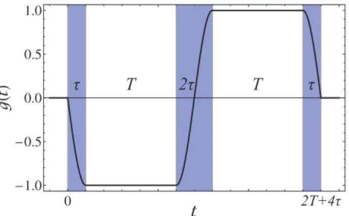
(29) g(t) = ⎧ ⎪ ⎪ ⎪ ⎪ ⎪ ⎪ ⎪ ⎨ ⎪ ⎪ ⎪ ⎪ ⎪ ⎪ ⎪ ⎩ − sin(Ωefft) 0 < t ≤ τR, −1 τR< t ≤ T + τR, − sin)Ωeff(t − T )* T + τR< t ≤ T + 3τR, 1 T + 3τR< t ≤ 2T + 3τR, − sin)Ωeff(t − 2T )* 2T + 3τR< t ≤ 2T + 4τR, 0 otherwise.

This function is illustrated in fig. 5.

3.1. Interferometer response to laser phase noise. – It is interesting to understand how this interferometer responds to phase noise at a given frequency. Recall that the standard deviation of interferometer phase noise, σrms

Φ , is composed of a sum over the laser phase

noise harmonics, Sφ(ω), weighted by |H(ω)|2 [see eq. (25)]. Thus, to investigate the

interferometer response to phase noise, we first compute the transfer function, H(ω), using eqs. (23), (24) and (29):

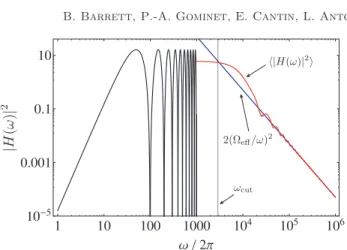
(30) H(ω) = 2iωΩeff ω2_{− Ω}2 eff % sin)ω(T + 2τR)* + 2Ωeff ω sin # ωT 2 $ sin# ω(T + 2τR) 2 $& . An example of the weight function, |H(ω)|2_{, is displayed in fig. 6, which has two important}

features. First, for frequencies much less than the Rabi frequency (ω * Ωeff), the transfer

function can be approximated by

(31) H(ω) ≈ −4i sin2# ω(T + τ₂ R)

$ ,

τ

T

2τ

T

τ

2T+4τ

Fig. 5. – (Colour online) Plot of the sensitivity function, g(t), for the three-pulse interferometer given by eq. (29). The pulse duration, τ , satisfies Ωeffτ = π/2.

which originates from the second term in eq. (30). In this regime, the weight function oscillates periodically, with zeroes at integer multiples of the fundamental harmonic: f0=

(T +τR)−1. Thus, the interferometer is relatively insensitive to phase noise at frequencies

much less than f0, since the weight function scales as |H(ω)|2∼ ω4(T +τR)4* 1. Second,

for frequencies ω ) Ωeff, the transfer function is dominated by the first term in eq. (30):

(32) H(ω) ≈ 2iΩeff

ω sin)ω(T + 2τR)*.

This expression indicates that there is a natural low-pass filtering of the higher harmonics due to the finite duration Raman pulses. As a result, the sensitivity of the interferometer to high-frequency phase noise scales as (Ωeff/ω)2, with an effective cut-off frequency at

ωcut= Ωeff/

√

3. These features have been confirmed experimentally in ref. [58].

In order to correctly evaluate the sensitivity of the interferometer to phase noise, it is necessary to take into account the fact that interferometer measurements are pulsed cyclically at a rate fc= 1/Tc. A natural tool to characterize the sensitivity is the Allan

variance of the atom interferometric phase fluctuations:

(33) σ_Φ2(τavg) = 1 2n→∞lim / 1 n n " k=1 ) ⟨δΦk+1⟩ − ⟨δΦk⟩ *2 0 ,

where ⟨δΦk⟩ is the mean value of δΦ over the measurement interval [tk, tk+1= tk+ τavg]

of duration τavg, which is an integer multiple of the cycle time: τavg = mTc. For large

enough averaging times τavg, where the fluctuations between successive averages are not

correlated, the Allan variance can be shown to be

(34) σ_Φ2(τavg) = 1 τavg ∞ " n=1 |H(2πnfc)|2Sφ(2πnfc).

Fig. 6. – (Colour online) Plot of the phase noise weight function, |H(ω)|2_{, for the three-pulse}

interferometer with T = 10 ms, τR = 50 µs and Ω_eff = π/2τR = 2π × 5 kHz. Here, the

black curve indicates |H(ω)|2_{, which has been terminated at 1 kHz. The red curve shows the}

average of |H(ω)|2 _{over one period of oscillation, (T + τ}

R)−1. In blue is the scale factor for

the weight function at large frequencies, 2(Ωeff/ω)2. The gray vertical line shows the effective

cut-off frequency of |H(ω)|2at ωcut= Ωeff/

√

3 ∼ 2π × 2.9 kHz.

This expression indicates that the sensitivity of the interferometer is limited by an aliasing phenomenon similar to the Dick effect for atomic clocks [57]. Only the phase noise at harmonics of the cycling frequency fc contributes to the Allan variance, and they are

weighted by the square of the transfer function at these frequencies.

3.2. Sensitivity to mirror vibrations. – The sensitivity function can also be used to investigate the response of the interferometer to motion of the retro-reflection mirror that acts as the inertial reference frame for absolute measurements of inertial effects. In this case, the phase noise can be expressed as φ(t) = keff· r(t), where r(t) represents the

time-dependent position of the mirror. Using eq. (22), the change in the interferometer phase due to mirror motion is

(35) δΦv=

! ∞

−∞

g(t)k_eff· v(t)dt,

where v(t) = ˙r(t) is the velocity of the mirror. Using the chain rule, eq. (35) can be converted to a more useful form:

(36) δΦa= −keff· 1 f (t)v(t)2∞ −∞ + k_eff· ! ∞ −∞ f (t)a(t)dt.

Here, a(t) = ˙v(t) is the acceleration noise of the mirror and f (t) is called the response function of the interferometer, which is defined as

(37) f (t) = − ! t 0 g(t′ )dt′ .

τ

T

2τ

T

τ

2T+4τ

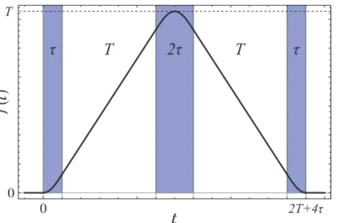
Fig. 7. – (Colour online) Plot of the response function, f (t), given by eq. (38). Again, the pulse duration satisfies Ωeffτ= π/2.

In what follows, we will illustrate how f (t) characterizes the sensitivity of the three-pulse interferometer to mirror vibrations. Integrating the sensitivity function given by eq. (29), we find (38) f (t) = ⎧ ⎪ ⎪ ⎪ ⎪ ⎪ ⎪ ⎪ ⎨ ⎪ ⎪ ⎪ ⎪ ⎪ ⎪ ⎪ ⎩ 1

Ωeff)1 − cos Ωefft

*

0 < t ≤ τR,

t + 1

Ωeff − τR τR< t ≤ T + τR,

T +_Ω1eff)1 − cos Ωeff(t − T )

*

T + τR< t ≤ T + 3τR,

2T + 3τR+_Ω1_eff − t T + 3τR< t ≤ 2T + 3τR, 1

Ωeff)1 − cos Ωeff(t − 2T )

*

2T + 3τR< t ≤ 2T + 4τR,

0 otherwise.

The response function for the three-pulse interferometer is a triangle-shaped function with units of time, as shown in fig. 7. Since it is equal to zero outside of the interval t ∈ [0, 2T + 4τR], the first term in eq. (36) vanishes and the phase variation of the

interferometer due to the acceleration noise of the mirror is

(39) δΦa= keff·

! ∞

−∞

f (t)a(t)dt.

At its heart, this expression is a generalization of the phase shift keff· aT2 produced by

atoms moving in a non-inertial reference frame with a constant acceleration.(7_{) Here,}

f (t) acts as a weight function that determines how strongly the mirror acceleration at time t contributes to the interferometer phase shift. The phase contributions are smallest

(7) Equation (39) can be evaluated with a constant acceleration to obtain: δΦa= k_eff · a(T +

2τR)(T + 4τR/π), which reduces to the well-known result k_eff· aT2in the limit of short Raman

Count 40 80 120 20 0 (a) !6 !4 !2 0 2 4 0.3 0.4 0.5 0.6 0.7 ∆#a!rad" Probability !arb. units " (b)

Fig. 8. – (Colour online) (a) Transition probability of a three-pulse 87Rb interferometer with total interrogation time 2T = 6 ms, measured in the presence of strong Raman mirror vibrations (standard deviation of acceleration noise: σa∼ 1.4 × 10−3 g). The data are plotted

chronologi-cally. On the left is a histogram of the measured probabilities, which resembles the probability distribution of cos−1(φ). The double-peaked structure indicates that the interferometer is op-erating normally, but the Raman phase is randomized by the mirror vibrations. (b) Same data as shown in (a) plotted as a function of the acceleration-induced phase, δΦa, given by eq. (39).

The tidependent acceleration, a(t), was recorded for each shot of the experiment with a me-chanical accelerometer (Colibrys SF3600A) attached to the Raman mirror. These data clearly show that the interferometer fringes can be reconstructed with a high degree of accuracy even in noisy environments.

near t = 0 and 2T + 4τR, where the wavepacket separation is a minimum. Similarly, the

weight is strongest near the mid-point, t = T + 2τR, where the separation between the

interfering states is a maximum.

Equation (39) suggests that, if the acceleration of the retro-reflecting mirror is mea-sured during the interferometer pulse sequence, one can correct for changes in the mirror position that induce parasitic phase shifts on the atoms. This principle is illustrated in fig. 8, where the initially randomized signal from a Mach-Zehnder interferometer in a noisy environment is recovered using the aforementioned analysis. Here, the fringes are effectively “scanned” by vibrations on the retro-reflecting Raman mirror. This has also been demonstrated with a mobile matter-wave interferometer in a micro-gravity environment during parabolic flights onboard a zero-g aircraft [59]. We give a detailed description of this experiment and recent results in sect. 5.3.

4. – Inertial sensors based on atom interferometry

In general, an inertial sensor is a device that can detect changes in momentum, for example, a change in direction caused by rotation, or a change in velocity caused by the presence of a force. High precision inertial sensors have found scientific applications in the areas of general relativity, geophysics and geology, as well as industrial applications, such as the non-invasive detection of massive objects, or oil and mineral prospecting.

theo-Fig. 9. – (Colour online) The atomic-fountain-based gravimeter developed by the Chu group at Stanford during the 1990’s [19, 52, 39]. On the right is a two-day recording of the variation of gravity. The high accuracy enables ocean loading effects to be observed. Photo courtesy of S. Chu and M. Kasevich.

retical and experimental studies were carried out to investigate these new kinds of inertial sensors [22]. To date, ground-based experiments using atomic gravimeters (measuring acceleration) [52, 39, 60, 61, 62], gravity gradiometers (measuring acceleration gradients) [63, 64, 62] and gyroscopes (measuring rotations) [65, 66, 67] have been realized and proved to be competitive with existing optical or artifact-based devices.

In this section, we present a brief summary of different inertial sensors based on atom interferometry that were designed as proof-of-principle experiments for use only in the laboratory. A classic example of such an experiment is the gravimeter developed at Stanford in the early 1990s shown in fig. 9. Later, in sect. 5, we focus on projects designed for “field” use and give detailed descriptions of some mobile sensors developed by our research groups.

4.1. Accelerometers and gravimeters. – If the three light pulses of the interferometer sequence are separated only in time, and not in space, the interferometer is in an ac-celerometer (or gravimeter) configuration. For a uniform acceleration a, in the atom’s frame the frequency of the Raman lasers changes linearly with time at a rate of −keff· a.

The resulting phase shift that arises from the interaction between the light and the atoms can be shown to be (see sect. 2)

(40) Φa = keff· aT2+ (φ1− φ2+ φ3).

Similarly, if the Raman beams are oriented along the vertical, the gravitationally induced chirp on the Raman frequency is −keff· g. In this case, the usual procedure to measure

g is to chirp the frequency of the Raman beams during the pulse sequence, such that the Doppler frequency of the atoms is canceled. The chirp rate, α, that compensates the

Fig. 10. – (Colour online) Transition probability as a function of the Raman beam chirp rate, α, for T = 50 ms. Taken from ref. [68].

Doppler shift is determined by the relation [68]

(41) Φg= (keff· g − α)T2= 0.

This expression can be obtained from eq. (40) by setting the phases, φj= φ(tj) = −αt2j/2,

where tj is the onset time of each pulse. The transition probability of the interferometer

then oscillates sinusoidally as a function of Φg, as shown in fig. 10. The central fringe,

for which α = k_effg, stays fixed for all values of T .

It should be noted that the phase shifts given by eqs. (40) and (41) do not depend on the initial atomic velocity or on the mass of the particle—a direct consequence of the equivalence principle. The first precision cold atom gravimeter [39] achieved a resolution of 20 µGal (1 µGal = 10−9_{g) after one measurement cycle lasting 1.3 s. When compared}

to the best classical devices (such as the Scintrex FG5, which is based on optical inter-ferometry with a falling corner cube), the two values of g agreed to within 7 µGal after accounting for systematic effects.

More recently, a comparison between three different gravimeters [69], one based on atom interferometry and two based on different optical technology, has shown agreement at the level of ∼ 25 µGal. Although this is outside the individual precision of any one instrument, the difference is expected to be caused by systematic effects that require further investigation.

The main limitation of this kind of gravimeter on Earth is due to spurious accel-erations of the reference platform. One possibility for overcoming this problem is to measure the vibration of the platform using a sensitive mechanical accelerometer and correcting for phase fluctuations either in post-analysis or in real-time, as we will discuss

1.4 m

Fig. 11. – (Colour online) Gravity gradiometer developed in Stanford [64]. This system was also used for measurements of the Newtonian constant G (see ref. [41]) using a 540 kg mass shown at the top of the photo on the left. Photos courtesy of M. Kasevich.

in sect. 5.3. Another option is to perform simultaneous measurements with two different atomic samples with the same reference platform. This offers the possibility of rejecting any common-mode vibration noise on the measurements [70, 71]. Furthermore, if the two samples are spatially separated, simultaneous measurements would be sensitive to spatial gradients in g, and would also allow one to suppress a variety of systematic effects. We discuss such an apparatus in the next section.

4.2. Gradiometers. – Measurements of the gradient of gravitational fields have impor-tant scientific and industrial applications ranging from the measurement of the Newtonian constant of gravity, G, and tests of general relativity, to covert navigation, underground structure detection, and geodesy. Initially at Stanford University, the development of atom-interferometric gravity gradiometers has been followed by other advances either for Space or fundamental physics measurements [60, 41, 42]. A crucial aspect of every design is its intrinsic immunity to spurious accelerations.

The gradiometer setup is illustrated in fig. 11. It measures, simultaneously, the ac-celeration of two separate laser-cooled ensembles of atoms. The geometry is chosen so that the measurement axis passes through both atomic samples. Since the acceleration measurements are made simultaneously at both positions, many systematic measure-ment errors, including the vibration of the experimeasure-mental platform, are common to both measurements and can be subtracted. The relative acceleration of the two ensembles along the axis defined by the Raman beams is measured by subtracting the measured phase shifts Φ(r1) and Φ(r2) at the two locations r1 and r2. The gradient is extracted

by dividing the relative acceleration by the separation of the ensembles. However, this method determines only one component of the gravity gradient tensor.

This type of instrument is fundamentally different from state-of-the-art classical sen-sors that are designed, for example, to measure G. First, the proof-masses are individual atoms rather than precisely machined macroscopic objects. This reduces systematic ef-fects associated with the material properties of these objects. Second, the calibration for the two accelerometers is referenced to the wavelength of a single pair of frequency-stabilized laser beams, and is identical for both accelerometers. This provides long term accuracy. Finally, large separations () 1 m) between accelerometers are possible, en-abling the development of high-sensitivity instruments. The apparatus shown in fig. 11, with a separation of 1.4 m, has demonstrated a differential acceleration sensitivity of 4 × 10−9_g/√_{Hz, corresponding to gravity-gradient sensitivity of 4 E/}√_{Hz (1 E = 10}−9

s−2_{) [64].}

More recently, a compact gravimeter (consisting of just one atomic source) measured the vertical gravity gradient with a precision of 4 E [62]. This was done by placing the instrument on an elevator and measuring g at various heights both above and below ground level.

4.3. Gyrometers. – In the case of a spatial separation of the laser beams, and when the atoms have a velocity component perpendicular to k_eff, the interferometer is in a configuration similar to an optical Mach-Zehnder interferometer. Then, in addition to accelerations, the interferometer is also sensitive to rotations. This is the matter wave analog to the optical Sagnac effect. For a Sagnac loop enclosing an area A, a rotation Ω produces a phase shift (to first order in Ω) of

(42) ϕrot=

4π

λdBvlΩ · A.

Here, λdBis the de Broglie wavelength and vlthe atom’s longitudinal velocity. The area

A of the interferometer depends on the distance between two light pulses, L, and on the transverse velocity vt= !keff/M :

A = L2vt vl

.

For the Mach-Zehnder atom interferometer, the phase shift due to the rotation takes the same form as that of an acceleration, except the free evolution time becomes T = L/vl

and the acceleration becomes acor= −2(Ω × v) (the Coriolis acceleration)

(43) Φrot= keff· acor

# L vl

$2

+ (φ1− φ2+ φ3).

By utilizing the small de Broglie wavelength of massive particles, atom interferometers can achieve a much higher sensitivity to rotations than optical interferometers with the same area. An atomic gyroscope [65, 66], using thermal caesium atomic beams (where

the most-probable longitudinal velocity was vl ∼ 300 m/s) and with an overall

inter-ferometer length of 2 m has demonstrated a sensitivity of 6 × 10−10 _rad/s/√_{Hz. The}

apparatus consists of a double interferometer using two counter-propagating sources of atoms, sharing the same lasers. The use of the two sources facilitates the discrimination between rotation and acceleration signals.

4.4. Six-axis sensor . – The sensitivity axis of an interferometer is usually defined by the direction of the Raman interrogation laser with respect to the atomic trajectory. An experiment carried out in Paris [67] demonstrated sensitivity to three mutually orthog-onal accelerations and rotations by launching two atomic clouds in opposite parabolic trajectories. As illustrated in fig. 12(a), with the usual π/2 − π − π/2 pulse sequence, a sensitivity to vertical rotation Ωz and to horizontal acceleration ay can be achieved by

placing the Raman lasers along the y-direction, perpendicular to the atomic trajectory. With the same sequence, using vertically-oriented lasers, the horizontal rotation Ωy and

vertical acceleration azcan be measured, as shown in fig. 12(b). The phase shift in these

two cases can be shown to be

(44) Φ3p= keff ·'a − 2(Ω × v)( T2.

It is also possible to access the other components of acceleration and rotation which lie along the x-axis (in the plane of the atomic trajectories). By utilizing these strongly curved launch trajectories, Raman lasers can be aligned along the x-direction—producing a sensitivity to the acceleration component axbut not to rotations [see fig. 12(c)]. Access

to the horizontal rotation Ωx is achieved by changing the pulse sequence along the

y-direction to a four-pulse “butterfly” configuration [see fig. 12(d)]. This configuration was first proposed to measure gravity gradients [64]. It involves four pulses with areas π/2 − π − π − π/2, and separated by times T/2 − T − T/2, respectively. The projection of the interferometer area along the x-axis gives rise to a sensitivity to the x-component of rotation, Ωx, described by the phase shift

(45) Φ4p=

1

2'keff× (g + a)( · Ω T

3_.

In contrast, the z-axis projection of the area cancels out, so the interferometer is insen-sitive to Ωz.

5. – Compact and mobile inertial sensors

Until now, we have discussed various applications of atom interferometry in terms of lab-based inertial sensors. These experiments are typically quite large, require a dedicated laboratory, and are designed to stay in one place. Furthermore, it is normal for sensors of this kind to operate well only in environments where the temperature, humidity, acoustic noise, etc.is tightly constrained. In this section, we describe three different projects that are designed to be compact, robust and mobile—making them distinctly

Fig. 12. – (Colour online) Six-axis inertial sensor. On the left is a schematic of the experimental setup, and typical operating parameters. On the right we illustrate the principle of operation. Here, two atomic clouds, labeled “A” and “B”, are launched on identical parabolic trajectories, but in opposite directions. The Raman lasers are pulsed on when the atoms are near the vertex of their trajectories. Four different interferometer configurations (a)–(d) give access to the 3 rotations and the 3 accelerations.

different from most laboratory experiments. The development of this technology will help create a new generation of atomic sensors that can operate “in the field” under a broad range of environmental conditions.

5.1. MiniAtom: a compact and portable gravimeter . – Here, we present the realization of a highly compact, absolute atomic gravimeter called “MiniAtom”, which was devel-oped jointly by labs at SYRTE (Observatoire de Paris) and LP2N (Institut d’Optique d’Aquitaine). The main purpose of this work is to demonstrate that atomic interferome-ters can overtake the current limitations of inertial sensors based on “classical” technolo-gies for field and on-board applications in geophysics. We show that the complexity and volume of cold-atom experimental set-ups can be drastically reduced while maintaining performances close to state-of-the-art sensors—enabling such atomic sensors to perform precision measurements outside of the laboratory. As a feasible prototype, we chose to realize an absolute gravimeter to measure the acceleration of the Earth’s gravity, which can be used to support geophysical surveys. This work has played an important role in the development of commercial cold atom gravimeters, one of which we will discuss in sect. 5.2.

The major design features—the reduction of the sensor head size and the significant simplification of the laser module—rely on the use of an innovative hollow pyramid as the retro-reflecting mirror of quantum inertial sensors and a laser system based on telecom technologies. This design allows us to perform all the steps of the atomic measurement (laser-cooling, selection, interferometry and detection) with just a single laser beam [61]. In contrast, other atomic gravimeters require up to 9 different optical beams (six beams for the MOT, one pusher beam, one for interferometry, and one for detection) coming from multiple frequency sources. As we will show, this key component is responsible for

(a)

(b)

40

cm

Fig. 13. – (Colour online) (a) Schematic of a compact gravimeter with only one laser beam and a pyramidal reflector. (b) The MiniAtom apparatus. The total height of the sensor head is 40 cm.

the simplifications of both the sensor head and the laser system.

The concept of a single beam interferometer performed with a pyramidal retro-reflector [illustrated in fig. 13(a)] was validated on a previous experiment, as described in ref. [61]. In that work, approximately 107 87_{Rb atoms were loaded from a vapor in}

∼ 400 ms. This is followed by 20 ms of molasses cooling which brings the atoms to a temperature of ∼ 2.5 µK. A sequence of microwave and pusher-beam pulses selects the atoms in the state |F = 1, mF = 0⟩ at the beginning of their free-fall. Once the cloud

has fallen clear of the pyramid, the two vertically-oriented, retro-reflected Raman beams are used to perform a velocity selection, followed by the usual π/2 − π − π/2 interferom-eter scheme. After the Raman pulses, the relative population between the two hyperfine ground states is obtained using fluorescence detection. With an interrogation time of 2T = 80 ms, we demonstrated a relative sensitivity to g of 1.7 × 10−7_{within one second}

of data acquisition, and we have shown promising long-term relative stability with a noise floor below 5 × 10−9_.

The sensor head [shown in fig. 13(b)] consists of a 2 liter titanium vacuum chamber which is magnetically shielded by a single layer of mu-metal. The science chamber features several optical viewports to perform the atomic measurement sequence. Four indium-sealed rectangular windows are designed to measure the fluorescence of the atoms at the output of the interferometer. These viewports were made 10 cm long in order to adjust the trade-off between cycling-rate and sensitivity with respect to applications or environment. A maximum interrogation time of 100 ms for the interferometer is allowed, which is limited by the 15 cm height between the bottom viewport and the pyramidal reflector. To keep the design as simple as possible, we do not use any optics for imaging in the detection. Two sets of four 1 cm2 _{area photodiodes allow for 3% fluorescence}

MOT

Pyramidal

reflector

Fig. 14. – (Colour online) Image of the MiniAtom pyramidal MOT. The bright dot at the center is the fluorescence emitted by about 108 atoms of87Rb loaded from a background vapor.

resulted in a drastic reduction of the volume of the sensor head—it fits in a cylinder 40 cm high and 20 cm in diameter, as shown in fig. 13(b). In comparison, a separate transportable absolute gravimeter developed at SYRTE [72] has a sensor head that is 80 cm high and 60 cm wide. Figure 14 shows an image of the pyramidal MOT produced in the MiniAtom chamber.

The laser system was designed such that all the frequencies necessary for the gravime-ter are carried along a single optical path with one linear polarization state. A liquid crystal variable retarder plate (LCVR) from Meadowlark is used to control the polariza-tion state of the laser field reaching the science chamber at each step of the measurement. For the trapping and cooling stages, the LCVR creates a circular polarization from the incoming linear one so that after successive reflections on the faces of the pyramid, light is in the σ+_/σ− _{configuration. For the interferometer, the polarization is then changed}

to a linear state aligned at 45◦ _{to the edges of the pyramid so that the two}

counter-propagating Raman beam polarizations are perpendicular. Just after the third Raman pulse, the polarization is switched back to circular to perform the state detection. An important feature of the reflector is that the faces of the pyramid have a special dielec-tric coating that prevents the two crossed polarizations to dephase from each other after successive reflections.

For this project, we developed a compact laser architecture (see fig. 15) based on telecommunication technology with one key element: a periodically-poled lithium-niobate (PPLN) wave-guide (from NTT Electronics, Japan) which is used to frequency-double the 1560 nm laser source to 780 nm via second harmonic generation. This method of frequency doubling using a waveguide is particularly efficient, because the confinement of the optical mode within the guide leads to a conversion efficiency as high as 50%. The telecom laser source is a cheap and convenient distributed feedback (DFB) laser diode.

A common laser architecture adopted in cold atom experiments is the master-slave configuration, where one fixed-frequency laser serves as a reference for multiple “slave” lasers whose frequencies are shifted relative to the “master”. In this experiment, we use

DFB PPLN Sat. Abs. Electronics φ PPLN φ FP EDFA φ ω νSA ω ν±SA 2 ±ω νSA νMOT νRepump

ω ν±MOT ω ν+MOT ω ν+MOT

ω ν+MOT±νRepump

2 +2ω νMOT

2 +2ω νMOT±νRepump

Feedback

signal

Fig. 15. – (Colour online) Architecture of the fiber-based laser system with only one laser diode. Quantities in blue represent the laser frequency at different parts of the optical chain, while quantities in green are modulation frequencies sent to the phase modulators. The modulations νMOT and νrepump are set such that two output frequencies serve as the MOT and repump

beams during the loading sequence, and they are adjusted to serve as the two Raman beams during the interferometry sequence. DFB = distributed feedback laser diode; ϕ = electro-optic phase modulator; FP = Fabry-Perot interferometer; PPLN = periodically-poled lithium niobate waveguide; EDFA = erbium-doped fiber amplifier; Sat. Abs. = saturated absorption spectrometer.

only one laser with a fixed optical frequency. The light from the DFB is split into two parts. A small amount of power is diverted to an electro-optic phase modulator (EOM) that shifts the laser frequency in such a way that, after doubling, the light is resonant with the F = 3 → F′ _{= 4 transition in}85_{Rb. It is then sent to a saturated absorption cell. The}

locking signal is deduced from synchronous detection at 5 MHz where the modulation is created using the same EOM. The second part of the DFB output is sent through another phase modulator driven by an independent yttrium iron garnet (YIG) oscillator whose detuning will be close to the F = 2 → F′ _{= 3 transition in}87_{Rb after}

frequency-doubling. The light is then filtered by a fiber-based Fabry-Perot cavity such that only one sideband remains. The frequency agility is supported by the very fast response of the EOM that enables the detuning for cooling and then for the Raman transition at ∼ 1 GHz to the red of the transition. A third fiber-based EOM is used to create a second frequency that will be close to the F = 1 → F′ _{= 2 transition for repumping during}

the trapping stage or for the second Raman frequency during the interferometer. The beam carrying these two frequencies is then amplified by an erbium-doped fiber amplifier (EDFA) to produce enough power to obtain a sufficient frequency-doubling conversion efficiency. With this setup, we obtain an output power of 200 mW at 780 nm after fiber-coupling. This scheme allows us to change the frequency spacing in the optical domain by adjusting the rf modulation, which is accomplished almost instantaneously. As a result, the laser frequency can be rapidly controlled without changing the current of the laser diode.

Particular efforts have been made to integrate the frequency chain used to derive the 6.835 GHz reference for both the optical Raman transitions and the microwave pulse used

(b) (a) Time (hrs) g -980560198 ( Gal) μ

Fig. 16. – (Colour online) (a) Prototype of a commercial absolute quantum gravimeter. The laser and control electronics are shown in the 19 inch racks on the upper right. The gravimeter is surrounded by a layer of mu-metal to shield from external magnetic fields. (b) Preliminary measurements from the prototype taken over several hours (uncorrected for systematic effects). Here, the total interrogation time is 2T = 100 ms, and the solid line is an overlayed tidal model that includes solid Earth and ocean-loading effects. The sensitivity is currently a few µGal after 1000 seconds of integration. Photo and data courtesy of µQuanS.

for the quantum state selection. Although our frequency chain fits in a 2 liter volume, it features a phase noise that limits the sensitivity to gravity only at the level of 10−7_m/s2

in one second. This is on the order of the best sensitivities achieved in the laboratory with the same interrogation time. Thus, this project has demonstrated an interesting trade-off between integration in a small package and a satisfying level of phase noise.

This prototype demonstrates that several mature pieces of technology can be gathered to produce precise measurements in a compact inertial sensor. Further work is being carried out to improve and simplify the filtering of ground vibrations. In addition, our sensor opens new doors toward the operation of an adjustable remote head gradiometer. 5.2. Toward a commercial absolute quantum gravimeter . – As a result of the research involved with the MiniAtom project at two French laboratories (SYRTE in Paris and LP2N in Bordeaux), a commercial absolute quantum gravimeter is currently being de-veloped for various applications in geophysics, including volcano monitoring, hydrology, and hydrocarbon and mineral exploration. The operational requirements for these ap-plications are extremely stringent, but modern telecom laser technology presents very attractive features for the development of a high-performance absolute gravimeter com-patible with field use.

The general architecture of the instrument is very similar to the one used in the MiniAtom experiment—it relies on the utilization of a pyramidal reflector, which enables all of the operations involved in the measurement sequence (cooling, interferometry, and detection) to be performed with a single laser beam. A strong technological effort was conducted in order to integrate the laser system required for the quantum manipulation

of atoms and the driving electronics. The laser system is based on the utilization of a fiber-based telecom laser operating at 1560.48 nm, which is then amplified and frequency-doubled to the required wavelength of 780.24 nm. This compact design is extremely robust and reliable. A prototype of the gravimeter is shown in fig. 16, along with some preliminary gravity measurements taken over several hours.

5.3. ICE: A mobile apparatus for testing the weak equivalence principle. – The ICE experiment (an acronym for Interf´erometrie atomique `a sources Coh´erentes pour l’Espace, or coherent atom interferometry for Space) is a compact and transportable dual-species atom interferometer. The main goal of ICE is to test the weak equivalence principle (WEP), also known as the universality of free-fall, which states that two massive bodies will undergo the same acceleration from the same point in space, regardless of their mass or internal structure. This principle is characterized by the E¨otv¨os parameter, η, which is the difference between the acceleration of two bodies, a1and a2, divided by their average

acceleration:

(46) η= 2a1− a2

a1+ a2.

Historically, there have been a number of experiments to test the WEP using classical bodies. The most precise tests have previously been carried out using lunar laser ranging [73], or using a rotating torsion balance [74], and have measured η at the level of a few parts in 1013. Although these previous tests are very accurate, they were both done with classical objects. Various extensions to the standard model of particle physics have made predictions that would directly violate Einstein’s equivalence principle [75], therefore it is interesting to test the WEP with “quantum bodies”.

ICE aims to measure η using a dual-species atom accelerometer that utilizes laser-cooled samples of 87_{Rb and} 39_{K [76, 59]. By performing simultaneous measurements}

on the two spatially-overlapped atomic clouds, the acceleration of the two species can be measured and common-mode noise can be rejected. This concept is similar to the operation principle of gradiometers, as we discussed in sect. 4.2.

The experiment is designed to perform this test in a micro-gravity environment (on-board the Novespace A300 “zero-g” aircraft) in order to extend the interrogation time, thereby increasing the sensitivity to acceleration. Similar research is being carried out in a lab-based experiment by a team in Paris that recently demonstrated a differential free-fall measurement at the level of 1.2 × 10−7_{g using a dual-species accelerometer with} 85_{Rb and}87_{Rb [71].}

Other Earth-based atom interferometry experiments that exploit long interrogation times are taking place around the world. Two examples include the QUANTUS (Quan-tengase Unter Schwerelosigkeit — Quantum gases under micro-gravity) experiment [77, 78] at the ZARM drop tower in Bremen, Germany, and at Stanford University in a recently constructed 10 m vacuum chamber [79, 80]. However, the defining feature of interferometry experiments like ICE and QUANTUS is that the apparatus is designed to be in free-fall with the atoms.

Fig. 17. – (Colour online) Top figure: schematic of a parabolic flight in the zero-g A300 airbus, courtesy of Novespace. Bottom figure: the ICE team in micro-gravity. From top to bottom: B. Barrett, B. Battelier, and P.-A. Gominet. Photo courtesy of the ESA and Novespace.

5.3.1. Parabolic flights. On average, ICE takes part in two parabolic flight campaigns per year, which are organized by Novespace (based out of Bordeaux-M´erignac airport), and are funded by the European Space Agency (ESA) and the French Space agency (CNES). Each campaign consists of three flights where the zero-g A300 aircraft undergoes multiple parabolic trajectories, as shown in fig. 17. Each flight typically contains 31 parabolas, and each of those consists of approximately 20 s of micro-gravity when the aircraft is in free-fall. This amounts to approximately 10 minutes of 0g per flight, or just over 30 minutes for the entire campaign.

During one parabola, the experiment has the potential of reaching a maximum inter-rogation time of 2T ∼ 20 s. In comparison, the QUANTUS experiment in the ZARM drop tower is currently limited to 2T = 4.7 s, with plans to extend this to 2T = 9.4 s when the tower is modified to accommodate a launched capsule [78]. Similarly, the 10 m