A global off-line model of size-resolved aerosol microphysics: I. Model development and prediction of aerosol properties

(1)

HAL Id: hal-00300913

https://hal.archives-ouvertes.fr/hal-00300913

Submitted on 14 Jan 2005

HAL is a multi-disciplinary open access

archive for the deposit and dissemination of sci-entific research documents, whether they are pub-lished or not. The documents may come from teaching and research institutions in France or abroad, or from public or private research centers.

L’archive ouverte pluridisciplinaire HAL, est destinée au dépôt et à la diffusion de documents scientifiques de niveau recherche, publiés ou non, émanant des établissements d’enseignement et de recherche français ou étrangers, des laboratoires publics ou privés.

A global off-line model of size-resolved aerosol

microphysics: I. Model development and prediction of

aerosol properties

D. V. Spracklen, K. J. Pringle, K. S. Carslaw, M. P. Chipperfield, G. W. Mann

To cite this version:

D. V. Spracklen, K. J. Pringle, K. S. Carslaw, M. P. Chipperfield, G. W. Mann. A global off-line model of size-resolved aerosol microphysics: I. Model development and prediction of aerosol properties. Atmospheric Chemistry and Physics Discussions, European Geosciences Union, 2005, 5 (1), pp.179-215. �hal-00300913�

(2)

ACPD

5, 179–215, 2005 Global aerosol microphysics model D. V. Spracklen et al. Title Page Abstract Introduction Conclusions References Tables Figures J I J I Back Close Full Screen / Esc

Print Version Interactive Discussion

EGU

Atmos. Chem. Phys. Discuss., 5, 179–215, 2005 www.atmos-chem-phys.org/acpd/5/179/

SRef-ID: 1680-7375/acpd/2005-5-179 European Geosciences Union

Atmospheric Chemistry and Physics Discussions

A global o

ff-line model of size-resolved

aerosol microphysics: I. Model

development and prediction of aerosol

properties

D. V. Spracklen, K. J. Pringle, K. S. Carslaw, M. P. Chipperfield, and G. W. Mann

The School of Earth and Environment, University of Leeds, UK

Received: 2 November 2004 – Accepted: 20 December 2004 – Published: 14 January 2005 Correspondence to: D. V. Spracklen (dominick@env.leeds.ac.uk)

(3)

ACPD

EGU

Abstract

A GLObal Model of Aerosol Processes (GLOMAP) has been developed as an exten-sion to the TOMCAT 3-D Eulerian off-line chemical transport model. GLOMAP simu-lates the evolution of the global aerosol size distribution using a sectional two-moment scheme and includes the processes of aerosol nucleation, condensation, growth,

co-5

agulation, wet and dry deposition and cloud processing. We describe the results of a global simulation of sulfuric acid and sea spray aerosol. The model captures features of the aerosol size distribution that are well established from observations in the ma-rine boundary layer and free troposphere. Modelled condensation nuclei (CN>3 nm) vary between about 250–500 cm−3 in remote marine boundary layer regions and

be-10

tween 2000 and 10 000 cm−3 (at standard temperature and pressure) in the upper tro-posphere. Cloud condensation nuclei (CCN) at 0.2% supersaturation vary between about 1000 cm−3 in polluted regions and between 10 and 500 cm−3in the remote ma-rine boundary layer. New particle formation through sulfuric acid-water binary nucle-ation occurs predominantly in the upper troposphere, but the model results show that

15

these particles contribute greatly to aerosol concentrations in the marine boundary layer. It is estimated that sea spray emissions account for only ∼10% of CCN in the tropical marine boundary layer, but between 20 and 75% in the mid-latitude Southern Ocean.

1. Introduction

20

Particles in the atmosphere contribute to radiative forcing directly by scattering and absorbing radiation, and indirectly by altering the properties of clouds. The latest In-tergovernmental Panel on Climate Change report (IPCC, 2001) estimated the direct forcing of anthropogenic aerosols to be −0.5 Wm−2 and the indirect forcing to lie be-tween 0 and −2 Wm−2. These forcings are comparable, but opposite in sign, to the

25

(4)

ACPD

EGU

The effect of changes in aerosol properties on clouds is a particularly uncertain quan-tity in climate simulations and also presents the greatest modelling challenge because of the many factors that control the links between aerosol properties and cloud prop-erties. The most fundamental, though by no means only, quantity that needs to be accurately prognosed in a model is the concentration of cloud condensation nuclei

5

(CCN) – the subset of the aerosol, usually the largest, that can form cloud droplets at a particular supersaturation. The CCN number depends on the concentration and composition of particles greater than about 50 nm dry diameter, which is a size range that is influenced by primary particle production and by secondary particles that have grown to this size through condensation and coagulation processes on the timescale

10

of days to weeks. The response of CCN concentrations to changes in the emissions of primary particles and precursor gases is therefore likely to be complex.

In order to make a better estimate of the indirect effect it is important to under-stand the factors that control the number of CCN at a given supersaturation in a cloud. However, early global aerosol models were not able to simulate the particle size

dis-15

tribution and only predicted the mass of certain particle classes, such as sulfate (e.g.,

Langner and Rodhe, 1991; Jones et al., 1994, 2001; Chin et al., 1996; Pham et al.,

1995;Feichtrer et al.,1997;Koch et al.,1999;Barth et al.,2000;Rasch et al.,2000) or carbonaceous material e.g., (Cooke and Wilson,1996; Tegen et al., 2000). Early climate simulations relied on empirical relationships between aerosol mass and CCN

20

concentration (e.g.,Jones et al.,1994,2001). Although such schemes are computa-tionally efficient for long climate change simulations and exploit the aerosol information in the model, they do not capture the dependence of cloud droplet concentration on aerosol properties that has been observed globally (Ramanathan et al.,2001). More recently models have been developed that are capable of a size-resolved description

25

of sea spray particles (Gong et al.,1997) and sulfate aerosol (Adams and Seinfeld,

2002). Development of size-resolved models of aerosol concentration brings with it the need to include the microphysical processes such as nucleation, condensation, coagulation and cloud processing that affect the size distribution. Although the global

(5)

ACPD

EGU

simulation of a fully size-resolved multicomponent aerosol is currently too numerically demanding for centennial scale climate model simulations, these models are essential tools for understanding what controls the microphysical – and ultimately the radiative and cloud-nucleating – properties of the global aerosol. As we show here, the evolution of the size distribution and the factors that control CCN can be examined on timescales

5

as short as 1 month, which is approximately the lifetime of the global aerosol.

This paper is the first of three papers describing a new GLObal Model of Aerosol Processes (GLOMAP). This first paper describes the model and the global simulations of aerosol properties. The second paper, in preparation, will examine in detail the sensitivity of the predicted aerosol size distribution to uncertainties in the driving

micro-10

physical processes. The third paper, in preparation, will present a detailed comparison of the model against aerosol observations. The GLOMAP model described here is currently restricted to sea spray and sulfate aerosol.

Section 2 gives a description of the model. Section 3 describes the simulated global fields of sulfur species. Section 4 describes the simulated global aerosol properties.

15

2. Model description

2.1. The TOMCAT chemical transport model

GLOMAP is an extension to the 3-D off-line Eulerian chemical transport model, TOM-CAT, which is described in e.g.Stockwell and Chipperfield(1999). TOMCAT is forced by meteorological analyses and can be run at a a range of resolutions and with

dif-20

ferent options for physical and chemical parameterisations. These options include a a comprehensive tropospheric chemistry scheme.

2.1.1. Meteorology

The model domain is global and the resolution used here is 2.8◦×2.8◦ latitude × lon-gitude with 31 hybrid σ-p levels extending from the surface to 10 hPa. The vertical

(6)

ACPD

EGU

geometric resolution varies from 60 m within the planetary boundary layer to 1 km at the tropopause. In the experiments performed here large-scale atmospheric transport is specified from European Centre for Medium-Range Weather Forecasts (ECMWF) analyses at 6-hourly intervals. Tracer advection is performed using the Prather ad-vection scheme (Prather,1986), which conserves second-order moments of the tracer

5

field. The non-local vertical diffusion scheme ofHoltslag and Boville(1993) calculates the planetary boundary layer height and eddy diffusion coefficients and is capable of representing convective turbulence. Sub-grid scale moist convection is parametrised using the scheme of Tiedtke (1989). Precipitation occurs due to sub-grid convective processes (also followingTiedtke,1989) and due to frontal (or large scale) processes

10

according to the scheme ofGiannakopoulos et al.(1999). 2.1.2. Gas phase chemistry

The chemical reactions included in the model are listed in Table 1. Concentrations of OH, NO₃, H₂O₂ and HO₂ are specified using 6-hourly monthly mean 3-D concen-tration fields from a TOMCAT run with detailed tropospheric chemistry and linearly

in-15

terpolated onto the model timestep. The chemical scheme in Table 1 is considered the minimum necessary to examine the sulfur cycle and sulfate aerosol formation. Time-dependent chemical rate equations are solved using the IMPACT algorithm of the ASAD software package (Carver et al.,1997).

GLOMAP includes SO₂ emissions from anthropogenic and volcanic sources and

20

dimethyl sulfide (DMS) emissions from the ocean. Anthropogenic emissions are taken from the Global Emissions Inventory Activity (GEIA) database (Benkovitz et al.,1996), which are seasonally averaged and based on the year 1985. In the baseline model runs presented here all the emitted sulfur is assumed to be SO₂, but in Spracklen et al. (in preparation, 2005)1 we also explore the sensitivity of modelled aerosol to

25

1_{Spracklen, D., Pringle, K., Carslaw, K., Chipperfield, M., and Mann, G.: A global off-line}

(7)

pro-ACPD

EGU

small amounts of primary sulfate aerosol. The emissions inventory classifies emissions as occurring above or below 100 m. The emissions are partitioned linearly onto the appropriate model grid levels according to the thickness of the model levels.

Oceanic DMS emissions are calculated using the monthly mean seawater DMS con-centration database ofKettle et al.(1999) and the sea-to-air transfer velocity ofLiss and

5

Merlivat (1986). The wind speed at 10 m, which is needed for the calculation of transfer velocity, is calculated from the ECMWF analyses used to force the model assuming a neutral surface layer and a roughness length of 0.001 m for the sea surface.

Volcanic emissions of SO₂ are obtained from Andres and Kasgnoc (1998) and in-jected at a constant rate between pressure levels of 880 and 350 hPa (Jones et al.,

10

2001). Sporadically erupting volcanoes are not included in the model. All volcanic emissions are assumed to be SO₂.

2.2. The aerosol microphysics module 2.2.1. The aerosol size distribution

The aerosol size distribution is simulated using the moving-centre scheme of

Jacob-15

son (1997a), which is often termed a two-moment sectional scheme. In this scheme the average mass per particle in each size section (or bin) as well as the total number concentration in the bin are carried (mass and number being the 2 moments). Within each section, the average particle size varies between the lower and upper bin edges as mass is added to, or removed from, the particles, for example due to condensation

20

and evaporation. If the average particle mass in a bin exceeds its fixed bin edge the total mass and number of particles in this bin is added to the appropriate new bin (not necessarily the adjacent one). The number concentration of the original bin is set to zero and its average mass re-set to the mid-point mass. Such a two-moment scheme explicitly describes the growth of a size distribution in terms of changes in the mass

25

of the particles in a bin. In contrast, in a single-moment number-only scheme growth cesses, Atmos. Chem. Phys. Discuss., in preparation, 2005.

(8)

ACPD

EGU

must be described in terms of the change in the number of fixed-size particles in each bin. Two-moment schemes have the advantage of greatly reducing the numerical di ffu-sion (in radius space) that is a characteristic of single-moment number-only schemes (Jacobson,1997a;Korhonen et al.,2003), but have the disadvantage in a 3-D model that two pieces of information need to be carried to define the size distribution of a

5

single-component aerosol. A multi-component, two-moment scheme results in a large increase in information needing to be carried. However, whilst the number of extra model tracers required to simulate the mass per particle in the two-moment scheme increases linearly with the number of chemical components in each particle only one number concentration is required for each distribution.

10

The bin centres are geometrically (mass ratio) spaced and span 0.001 to 25 µm equivalent dry diameter. The number of bins can be set arbitrarily, although the num-ber required to capture the principal features of the natural size distribution is about 20 (Gong et al.,2003), which we use here. Water is not included as an aerosol compo-nent. Instead, particles are allowed to re-equilibrate with the ambient relative

humid-15

ity before calculating size-dependent quantities such as the coagulation kernel. The model conserves aerosol number and aerosol mass.

2.2.2. Microphysical processes

These simulations are restricted to sulfuric acid aerosol (formed through gas-to-particle conversion of gaseous H₂SO₄) and sea spray. As a further simplification, these two

20

aerosol types are assumed to have the same physical properties (density and hygro-scopic behaviour) and their chemical properties are not simulated (that is, we do not calculate the chemical composition and cation/anion speciation of the particles). The chemical equilibration of mixed electrolytes is a complex and numerically expensive problem to solve in a global model (Jacobson,1997b) and the effects, in terms of

par-25

ticle size distribution, are likely to be subtle in most parts of the atmosphere.

The number of solute molecules per particle in each size bin is converted to a particle volume using the K ¨ohler equation appropriate for sulfuric acid-water mixtures and

(9)

rel-ACPD

EGU

ative humidities from the meteorological analyses. The assumption that the sea spray particles have the same hygroscopic properties as sulfuric acid will lead to a factor 1.33 difference in the diameter of the particles under humid oceanic conditions where most of the sea spray particles reside (Gong et al.,2003).

New particle formation is treated using the binary H₂SO₄-H₂O nucleation scheme of

5

Kulmala et al.(1998). New particles are assumed to nucleate at a size of 100 molecules of H₂SO₄per particle. Condensation of H₂SO₄onto all particles is calculated using the modified Fuchs-Sutugin equation (Fuchs and Sutugin,1971). The noncontinuum effect that occurs during condensation onto small particles is accounted for using a correction factor which is a function of the Knudsen number. The accommodation coefficient, a_e,

10

is assumed to have a value of unity, although the sensitivity of the aerosol distribution to the magnitude of a_eis explored in Spracklen et al. (in preparation, 2005)1.

Coagulation of particles is calculated using the mass conserving semi-implicit nu-merical solution ofJacobson et al. (1994). The coagulation kernels account only for Brownian diffusion, which is the dominant mechanism for submicron particles. Kernels

15

are calculated using the size of the particles after equilibration with water.

Dry deposition of aerosols is based on the schemes of Slinn and Slinn(1981) and

Zhang et al.(2001). It includes the deposition processes of gravitational settling, Brow-nian diffusion, impaction, interception and particle rebound.

In-cloud aqueous phase oxidation of SO₂ to form aqueous H₂SO₄ is calculated in

20

grid boxes that contain low stratiform cloud according to global fields from the Interna-tional Satellite Cloud Climatology Project D1 database (Rossow and Schiffer, 1999). We assume that particles with a dry diameter larger than 0.05 µm activate. The maxi-mum rate of aqueous oxidation is set by the rate of diffusion of SO2onto the activated particle distribution, which is calculated using the Fuchs-Sutugin equation (Fuchs and

25

Sutugin,1971). Available SO₂is reacted stoichiometrically with H₂O₂and the concen-trations of both are reduced accordingly. Sulfate is added to the particle distribution and partitioned between different size bins depending on the rates of SO₂diffusion to each particle size bin. If H₂O₂concentrations were allowed to return to the prescribed

(10)

ACPD

EGU

values at the end of each time step this would cause an overprediction of H₂O₂ oxi-dation rates. Instead H₂O₂ is replenished using the prescribed concentration of HO₂ (Jones et al.,2001).

The emission of sea spray particles is calculated using the parametrisation ofGong

(2003), which produces realistic emissions at particle sizes between 0.07 and 20 µm

5

at 80% humidity (corresponding to approximately 0.035 and 10 µm dry diameter). This parametrisation is an extension of the semi-empirical formulation of Monahan et al.

(1986) to below 0.2 µm diameter, where the original parametrisation was found to over-estimate emissions of sub-micron sea spray particles. The adjustable parameter (Θ) that controls sub-micron emissions is set at 30.

10

GLOMAP includes description of both in-cloud and below-cloud aerosol wet depo-sition (due to both convective and frontal precipitation). The in-cloud (or nucleation) scavenging scheme assumes a removal rate of activated aerosol that is proportional to the amount of condensate converted to rain in each timestep. Below-cloud scavenging (impaction by raindrops) is parameterised followingSlinn(1983) with scavenging

coef-15

ficients taken fromBeard and Grover(1974). The raindrop distribution is assumed to follow the Marshall-Palmer distribution (with the sophistication of Sekhon and

Srivas-tava,1971) and is described with seven geometrically spaced raindrop bins. 2.2.3. Numerical treatment

The differential equations that govern the particle mass and number concentration in

20

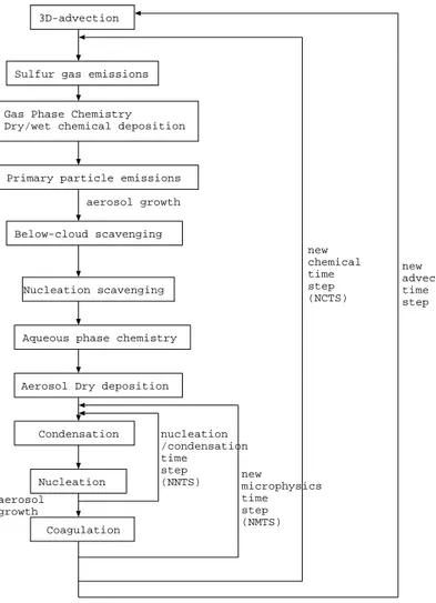
each size section are solved using operator splitting. This technique has been widely used in large-scale atmospheric models and has the advantage of being considerably cheaper in CPU usage compared to the fully coupled solution. The accuracy of the operator splitting depends on the length of the timestep used. A flowchart of the mi-crophysical operations in GLOMAP is shown in Fig.1. The TOMCAT model timestep is

25

split into a number of shorter subtimesteps that account for the time scales on which the different microphysical processes operate. The advection timestep is usually 1800 s. This is split into NCTS timesteps (normally 2) over which the emissions and

(11)

chem-ACPD

EGU

istry are solved. This timestep is then further split into NMTS timesteps (normally 2) over which the aerosol microphysics is solved. To accurately represent the competition between nucleation and condensation processes this microphysics timestep is subdi-vided further into NNTS timesteps (normally 5) where condensation and nucleation are calculated.

5

The accuracy of operator splitting has been tested by changing the length of the different timesteps and the order of operations. Changing the order of operations or further reducing the timestep length changes total aerosol number concentrations by less than 5%.

2.3. Model experiments

10

The runs were forced by ECMWF analyses. The model runs shown here are for De-cember 1995 and July 1997. The model was spun up from an aerosol-free atmosphere (on 1 October 1995 and 1 May 1997) for a period of 60 days before model output was used. This length of time is sufficient so that model simulations are independent of the model initialisation fields.

15

3. Global sulfur species

We now briefly describe the model fields of gaseous sulfur species as an aid to under-standing the distribution of aerosol in Sect.4.

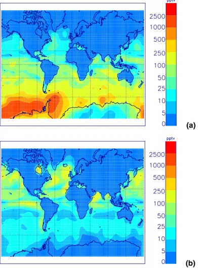
Figure 2 shows simulated surface level DMS concentrations. DMS concentrations are highest over oceanic areas (between 5 and 2000 pptv) due to oceanic DMS

emis-20

sions, and very low over terrestrial areas (less than 5 pptv). The model does not include any terrestrial emissions of DMS and so will tend to underpredict DMS concentrations over land. However, continental emissions of DMS are small and this should not be significant (Pham et al.,1995). The lifetime of DMS is approximately 1 day so its distri-bution is strongly governed by its sources, and atmospheric DMS concentrations in the

(12)

ACPD

EGU

marine boundary layer (MBL) closely follow the DMS concentrations in seawater. The simulations show the strong seasonal variability in atmospheric DMS concentrations caused by the cycle in biological activity altering sea surface DMS concentrations.

The largest simulated DMS concentrations occur over the tropical oceans and in the 30–60◦ oceanic belt of the summer hemisphere. This distribution reflects larger DMS

5

emissions in these regions, due to a combination of high ocean surface DMS con-centrations and higher wind speeds at the higher latitudes. Maximum values above the equatorial oceans of 300 pptv, and at high SH latitudes during the summer of over 1000 pptv, are calculated. Low DMS sea-surface concentrations in the winter hemi-sphere cause low DMS emissions and low winter hemihemi-sphere atmospheric

concen-10

trations. Coastal areas with strong oceanic upwelling (e.g., the Peru upwelling zone) have elevated DMS sea surface concentrations (Kettle et al.,1999) leading to higher atmospheric concentrations. Simulated gas phase DMS concentrations agree with measurements in both the Southern Ocean (e.g.Ayers et al.,1995;Shon et al.,2001;

Berresheim et al.,1990; De Bruyn et al.,1998;Nguyen et al.,1990) and tropical

re-15

gions (e.g.Bandy et al.,1996;Andreae et al.,1985) to within a factor of 2 to 3, which is reasonable considering the similar uncertainty in the gridded emissions (Kettle et al.,

1999) and sea-air transfer rates.

Figure3shows simulated surface level SO₂ concentrations. Concentrations of SO₂ are high over the United States, Europe and the Far East where there are large

emis-20

sions from fossil fuel burning. Additional maxima are observed over certain locations in Siberia and in the SH in Africa and South America due to smelting activities. The lifetime of SO₂is sufficiently long that transport of SO2away from these source regions is apparent, particularly from the east coast of the United States and the east coast of Asia. In December the model simulates strong advection of SO₂from Europe and the

25

United States to regions north of the Arctic circle. The aerosol mass loading is also greatly increased in Arctic regions affected by such transport of anthropogenic SO2 (see Sect.4).

(13)

ACPD

EGU

over the northern hemisphere (NH), with wintertime concentrations being a factor of two higher than summertime concentrations. This cycle has been explained by higher emissions (over Europe winter emissions in the GEIA inventory are about 30% higher than in summer), lower oxidant concentrations, and a stable boundary layer during win-ter months (Rasch et al.,2000). In clean marine areas SO₂concentrations of between

5

10 and 100 ppt are simulated, with the majority of the SO₂ deriving from DMS oxida-tion. Concentrations of SO₂ in the SH winter are very low due to low concentrations of DMS. The low concentrations of around 10 ppt in the tropics are due to efficient aqueous phase oxidation and removal in clouds. Simulated SO₂concentrations agree with measurements both over polluted continental regions (e.g., EMEP, 1989; Shaw

10

and Paur,1983;Heintzenberg and Larssen,1983;Barrie and Bottenheim,1990) and remote oceanic regions (e.g.,Ayers et al.,1997;De Bruyn et al.,1998;Bandy et al.,

1996) within a factor of 2 to 3.

4. Global aerosol properties

4.1. Global CN and CCN distributions

15

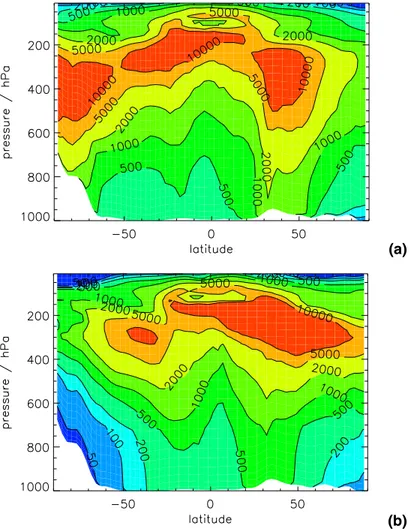
Figures4and5show surface and Figs. 6and7zonal mean simulated monthly mean number concentrations of condensation nuclei (CN) and cloud condensation nuclei (CCN). To allow easy comparison with observations CN are reported as the concen-tration of particles >3 nm diameter, which corresponds to the detection limit of current instruments (Stolzenburg and McMurry,1991). CCN are reported at 0.2%

supersatura-20

tion, which is typical of marine stratocumulus clouds, and corresponds to the activation of particles having a dry diameter of about 70 nm. All concentrations have been con-verted to conditions of standard temperature and pressure (STP, 273 K and 1 atm).

Smallest CN number concentrations are found in remote marine areas and largest concentrations are found near anthropogenically polluted regions. Simulated remote

25

(14)

obser-ACPD

EGU

vations (Clarke et al.,1987;Fitzgerald,1991;Andreae et al.,1994,1995;Pandis et al.,

1995;Covert et al.,1996;Raes et al.,2000). Over the United States, Europe and East and Central Asia surface CN number concentrations of around 1000–5000 cm−3 are simulated. This is somewhat lower than most observations under polluted continental conditions of 5×103and 1×105cm−3 (Raes et al.,2000;Pandis et al.,1995). A

pos-5

sible reason for this underprediction of CN concentrations over continental regions is discussed in Spracklen et al. (in preparation, 2005)1.

Simulated CN concentrations increase with altitude (Fig.6), with maximum concen-trations simulated in the upper troposphere (UT), as has been observed in recent field campaigns (e.g.,Clarke et al., 1999) and simulated in models (Adams and Seinfeld,

10

2002). Simulated UT concentrations in the tropics peak at higher concentrations and at higher altitudes than at mid latitudes.

Simulated CCN concentrations decrease with increasing altitude and concentrations are generally highest in polluted NH regions, with an obvious correlation between CN, CCN and sources of anthropogenic SO₂. Interestingly, CN concentrations are higher

15

in winter than summer while CCN concentrations show the opposite (though less pro-nounced) seasonal variation. In winter, lower temperatures mean that nucleation can occur over a greater depth of the free troposphere (FT), which leads to higher surface CN concentrations. In summer, higher OH radical concentrations lead to greater pro-duction of gas phase sulfuric acid, which causes faster rates of condensational growth

20

(while having little effect on the insignificant binary homogeneous nucleation rate). The lower number of available particles are able to grow faster, leading to higher CCN con-centrations. Also apparent in Fig.6 is the vertical extension of the CCN-rich air into the summer FT, which is caused by more efficient vertical mixing of boundary layer air. CCN concentrations are also clearly depleted along the Inter-Tropical Convergence

25

Zone (ITCZ) due to effective cloud scavenging processes.

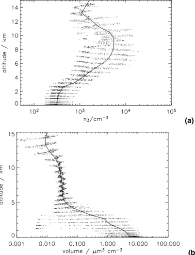
Figure 8 shows daily average altitude profiles of CN number and volume concen-tration over the remote South Pacific Ocean. Simulated CN concenconcen-trations increase by about an order of magnitude between the surface and 10 km altitude, as has been

(15)

ACPD

EGU

observed in a variety of field campaigns (e.g.Clarke and Kapustin,2002). Maximum CN concentrations at this location are simulated at around 9 km altitude. Simulated dry volume concentrations are greatest at the surface (1–15 µm3cm−3) and decrease with increasing altitude (to about 0.02–0.05 µm3 cm−3 at 10 km), as has been observed (Clarke and Kapustin, 2002). Figure 8 also gives an indication of the instantaneous

5

spatial variability in aerosol number and volume in a limited region. Notice, for exam-ple, the greater than 2 orders of magnitude variability in aerosol volume between 1 and 3 km altitude that arises due to cloud scavenging processes.

4.2. Contribution of sea spray to CCN

It is important to quantify the relative contribution of sea spray particles and other

10

aerosols to MBL CCN for several reasons. Firstly, oceanic regions have low natu-ral aerosol concentrations and are therefore susceptible to modification due to inputs from anthropogenic emissions. Secondly, the sea spray source function is particularly uncertain for particles with sizes less than 1 µm, and it is particles of this size that con-tribute most to the CCN number. Thirdly, the climate response to changes in emissions

15

of DMS depends on the changes in CCN resulting from new sulfate particles in the MBL.

The relative contribution of sea spray and sulfate particles to MBL CCN is uncer-tain and dependent on locations and atmospheric conditions. Blanchard and Cipriano

(1987) measured background MBL sea spray particle concentrations of between 15

20

and 20 cm−3. O’Dowd et al. (1999) observed that 10% of the accumulation mode aerosol was derived from sea spray particles in the Pacific Ocean MBL (600 km off the coast of California with wind speeds of less than 10 ms−1) and that about 30% of total aerosol concentration was sea salt in the North Atlantic MBL (with wind speed up to 17 ms−1). Yoon and Brimblecombe(2002) used a box model to predict that more than

25

70% of MBL CCN were derived from sea salt where wind speeds were moderate to high, especially in winter seasons in middle to high latitude regions.

(16)

ACPD

EGU

This was calculated by comparing a baseline model run with sulfate and sea spray sources to a run where only sea spray emissions were included. In our model simu-lations most of the sulfate aerosol formation and growth to CCN sizes occurs in low temperature regions lying well above the MBL, so our estimate of relative contributions to CCN based on two separate simulations is likely to be reasonable. More accurate

5

estimates will be possible in a multicomponent version of GLOMAP currently under development.

In the tropical oceanic MBL the model predicts that sea spray contributes less than 10% to total CCN. The remaining 90% are derived mostly from sulfate particles that formed in the free and upper troposphere. The importance of the UT as a source of

10

tropical MBL aerosol is apparent in a run in which aerosol nucleation was switched off below 3 km, which showed little change in MBL sulfate aerosol (not shown here). In the 30–60◦ oceanic belt sea spray generally contributes between 20 and 75% of total MBL CCN. In the continental boundary layer sea spray contributes less than 1% to total CCN.

15

4.3. Particle size distributions

The global aerosol distribution was simulated using 20 aerosol size bins. For simplicity, the results can be displayed as four typical size classes based on dry diameter (D_p): nucleation (D_p<7 nm), Aitken (7 nm<D_p<65 nm), accumulation (65 nm<D_p<700 nm)

and coarse particles (D_p>700 nm). Figures10 and 11 show surface level and zonal

20

mean aerosol concentrations divided into these four size ranges for December and July. These are typically accepted ranges that are convenient for dividing the aerosol distribution. However, it does not imply the presence of genuinely distinct modes in the modelled size distribution.

Coarse mode aerosol concentrations are much greater over oceanic areas because

25

these particles are derived from emission of sea spray. Large particles are subject to fast deposition rates and and are not advected far from their source regions, resulting in strong concentration gradients at land-ocean boundaries. Model emission rates

(17)

ACPD

EGU

of sea spray particles depend only on the surface wind speeds, resulting in largest MBL concentrations where wind speeds are fastest: generally in the 30–50◦S oceanic belt. Low concentrations are simulated near the equator due to the relatively low wind speeds there and the efficient removal of particles in tropical rain clouds.

Both coarse mode and accumulation mode concentrations are strongly depleted

5

along the ITCZ. This is caused by cloud scavenging and convective precipitation ef-fectively removing these larger particles. In contrast Aitken mode particles are not effectively removed by these processes as they do not serve as cloud condensation nuclei nor are they efficiently impaction scavenged by rain (Andronache,2003), so no depletion is obvious along the ITCZ.

10

As with seasonal variation of CN and CCN, in the NH winter Aitken mode concentra-tions are higher than in the NH summer whereas accumulation mode concentraconcentra-tions are higher in NH summer than NH winter. In the SH winter, concentrations of both Aitken and accumulation mode aerosol are reduced due to the lack of DMS emissions. The model simulates low concentrations of nucleation mode particles at the surface

15

and their distribution is much more patchy than other size classes. The MBL tends to have temperatures that are too high for H₂SO₄-H₂O binary nucleation to occur. Addi-tionally, the large pre-existing aerosol surface area near the surface means that most of the available H₂SO₄rapidly condenses onto the existing aerosol rather than forming new particles. In some marine areas concentrations of nucleation mode particles up

20

to 250 cm−3 are simulated. These tend to occur in regions of low FT temperatures. Rapid vertical mixing can transport nucleation mode particles produced in the FT to the surface before they grow through coagulation and condensation to larger particles. However, there is a clear absence of nucleation mode aerosol where sulfur sources are very limited (see Figs.2and3) even if FT temperatures are very low. This can be seen

25

over the Antarctic continent during the SH winter where no nucleation mode aerosol is simulated. Examination of daily fields of accumulation mode aerosol in remote marine areas reveals an anti-correlation between accumulation mode number and nucleation mode number (not shown here). This will be due to low accumulation mode number

(18)

ACPD

EGU

resulting in low pre-existing particle surface area which allows gas phase H₂SO₄ con-centrations to build up.

Nucleation and Aitken mode particle concentrations reach a maximum in the UT, with decreasing concentrations towards the surface. Downward transport of nucleation particles from the UT occurs simultaneously with their growth to Aitken mode

parti-5

cles, through coagulation and condensation. Accumulation mode and coarse mode particles have maximum concentrations at the surface. Coarse mode particles have a strong concentration gradient with altitude, with concentrations 103–104times lower at 400 hPa than at the surface. This is due to very efficient removal processes by dry and wet deposition. As the model does not simulate gravitational settling of large particles

10

from the upper to lower levels it is possible that the model overestimates the transport of large particles to higher altitudes. Accumulation mode particles are less efficiently removed and are transported to higher altitudes.

Figure 12 shows number and volume distributions as a function of dry particle di-ameter for December and July. For the North Atlantic MBL and FT, observed size

15

distributions fromRaes et al.(2000) are included for comparison. These observations are chosen as they are a climatology rather than measurements over a specific time period.

In the MBL the model captures the characteristic submicron bimodal number-size distribution (the smaller mode at about 20–80 nm diameter and the the larger mode

20

between 100–500 nm diameter) and an additional mode in the supermicron range (Fitzgerald,1991).

In the FT (at 2.3 km altitude) the model shows a typical FT unimodal distribution of particle concentration. However, comparison of model simulations with observations fromRaes et al.(2000) over the North Atlantic shows that the model tends to

empha-25

sise a large (sea spray) mode at >1 µm which is not distinct in the observations. The modelled North Atlantic size distribution is strongly perturbed by anthropogenic sulfur emissions, which, in both summer and winter, dominate the natural emissions. Aitken and accumulation mode particle concentrations greatly exceed those in the

(19)

ACPD

EGU

Southern Ocean where natural emissions dominate. The Southern Ocean nucleation and Aitken mode particles also show a lack of growth compared with those in the North Atlantic. Particle growth is even more limited in the Antarctic regions due to the very low sulfuric acid gas concentrations there.

5. Conclusions

5

A new global off-line aerosol microphysics chemical transport model incorporating a sectional treatment of the aerosol size distribution has been used to simulate the at-mospheric distributions of sulfur gases and sulfate and sea spray aerosol. The global tropospheric aerosol was created in the model by spinning up from an initially aerosol-free atmosphere over a period of 60 days. This period is long enough for the aerosol

10

size distribution in all parts of the atmosphere to become insensitive to the length of spin-up.

In the current configuration of the model we have simulated only sea spray and sul-fate aerosol, with the latter formed through binary homogeneous nucleation. The model simulates realistic MBL CN concentrations of 250–500 cm−3 over remote regions and

15

1000–5000 cm−3 immediately downwind of continental pollution sources. While CN concentrations in remote marine regions are broadly in agreement with observations, those in polluted regions are somewhat lower than suggested by observations. Pos-sible explanations for this disparity are examined in Spracklen et al. (in preparation, 2005)1. The UT and FT are the dominant source regions for new sulfuric acid particles

20

due to the low temperatures there, which accelerate the rate of binary homogeneous nucleation (Kulmala et al.,1998). These new particles grow through coagulation and condensation as they are transported downwards through the FT and provide a source of particles up to 100 nm dry diameter above the MBL. The FT particle size distribution is monomodal, while in the MBL the model simulates the typical trimodal distribution

25

with Aitken, accumulation and coarse modes occurring at approximately the correct sizes and number concentrations. The model supports the hypothesis that MBL

(20)

parti-ACPD

EGU

cle number is sustained by entraining particles which have nucleated in the FT.

References

Adams, P. and Seinfeld, J.: Predicting global aerosol size distributions in general circulation models, J. Geophys. Res.-A, 107, 4370–4393, 2002. 181,191

Andreae, M., Ferek, R., Bermond, F., Byrd, K., Engstrom, T., Hardin, S., Houmere, P.,

LeMar-5

rec, F., Raemdonck, H., and Chatfield, R.: Dimethyl sulfide in the marine atmosphere, J. Geophys. Res.-A, 90, 12 891–12 900, 1985. 189

Andreae, T., Andreae, M., and Schebeske, G.: Biogenic sulfur emissions and aerosol over the tropical South Atlantic, 1. Dimethylsulfide in seawater and in the atmospheric boundary layer, J. Geophys. Res.-A, 99, 22 819–22 829, 1994. 191

10

Andreae, M., Elbert, W., and de Mora, S.: Biogenic sulfur emissions and aerosols over the tropical South Atlantic, 3. Atmospheric dimethylsulfide, aerosols and cloud condensation nuclei, J. Geophys. Res.-A, 100, 11 335–11 356, 1995. 191

Andres, R. and Kasgnoc, A.: A time-averaged inventory of subaerial volcanic sulfur emissions, J. Geophys. Res.-A, 103, 25 251–25 261, 1998. 184

15

Andronache, C.: Estimated variability of below-cloud aerosol removal by rainfall for observed aerosol size distributions, Atmos. Chem. Phys., 3, 131–143, 2003,

SRef-ID: 1680-7324/acp/2003-3-131. 194

Atkinson, R., Baulch, D., Cox, A., Hampson Jr., R., Derr, J., and Troe, J.: Evaluated kinetics and photochemical data for atmospheric chemistry: Supplement III, J. Phys. Chem. Ref. Data,

20

88, 881–1097, 1989. 203

Ayers, G., Bentley, S., Ivey, J., and Forgan, B.: Dimethylsulfide in marine air at Cape Grim, 41◦ S, J. Geophys. Res.-A, 100, 21 013–21 021, 1995. 189

Ayers, G., Cainey, J., Gillett, R., Saltzman, E., and Hooper, M.: Sulfur dioxide and dimethyl sulfide in marine air at Cape Grim, Tasmania, Tellus, 49B, 292–299, 1997. 190

25

Bandy, A., Thornton, D., Blomquist, B., Chen, S., Wade, T., Ianni, J., Mitchell, G., and Nadler, W.: Chemistry of dimethyl sulfide in the equatorial Pacific atmosphere, Geophys. Res. Lett., 23, 741–744, 1996. 189,190

Barrie, L. and Bottenheim, J.: Pollution in the arctic atmosphere, chap. Sulphur and Nitrogen Pollution in the Arctic Atmosphere, 151–181, Elsevier, 1990. 190

(21)

ACPD

EGU

Barth, M., Rasch, P., Kiehl, J., Benkovitz, C., and Schwartz, S.: Sulfur chemistry in the Na-tional Center for Atmospheric Research Community Climate Model: Description, evaluation, features, and sensitivity to aqueous chemistry, J. Geophys. Res.-A, 105, 1387–1415, 2000. 181

Beard, K. and Grover, S.: Numerical collision efficiencies for small raindrops colliding with

5

micron size particles, J. Atmos. Sci., 31, 543–550, 1974. 187

Benkovitz, C., Scholtz, M., Pacyna, J., Tarras ´on, L., Dignon, J., Voldner, E., Spiro, P., Logan, J., and Graedel, T.: Global gridded inventories of anthropogenic emissions of sulfur and nitrogen, J. Geophys. Res.-A, 101, 29 239–29 253, 1996. 183

Berresheim, H., Andreae, M., Ayers, G., Gillett, R., Merrill, J., Davis, V., and Chameides, W.:

10

Airborne Measurements of Dimethylsulfide, Sulfur Dioxide, and Aerosol Ions over the South-ern Ocean South of Australia, J. Atmos. Chem., 10, 341–370, 1990. 189

Blanchard, D. and Cipriano, R.: Biological regulation of climate, Nature, 330, 526, 1987. 192 Carver, G., Brown, P., and Wild, O.: The ASAD atmsopheric chemistry integration package and

chemical reaction database, Computer Physics Communications, 105, 197–215, 1997. 183

15

Chin, M., Jacob, D., Gardner, G., Foreman-Fowler, M., and Spiro, P.: A Global three-dimensional model of tropospheric sulfate, J. Geophys. Res.-A, 101, 18 667–18 690, 1996. 181

Clarke, A. and Kapustin, V.: A Pacific Aerosol Survey, Part I: A Decade of Data on Particle Production, Transport, Evolution, and Mixing in the Troposphere, J. Atmos. Sci., 59, 363–

20

382, 2002. 192

Clarke, A., Ahlquist, N., and Covert, D.: The Pacific marine aerosol: Evidence for natural acid sulfates, J. Geophys. Res.-A, 92, 4719–4190, 1987. 191

Clarke, A., Eisele, F., Kasputin, V., Moore, K., Tanner, D., Mauldin, L., Litchy, M., Lienert, B., Carroll, M., and Albercook, G.: Nucleation in the equatorial free troposphere: Favorable

25

environments during PEM-Tropics, J. Geophys. Res.-A, 104, 5735–5744, 1999. 191 Cooke, W. and Wilson, J.: A global black carbon aerosol model, J. Geophys. Res.-A, 101,

19 395–19 409, 1996. 181

Covert, D., Kapustin, V., Bates, T., and Quinn, P.: Physical properties of marine boundary layer aerosol particles of the mid-Pacific in relation to sources and meteorological transport, J.

30

Geophys. Res.-A, 101, 6919–6930, 1996. 191

De Bruyn, W., Bates, T., Cainey, J., and Saltzman, E.: Shipboard measurements of dimethyl sulfide and SO2southwest of Tasmania during the First Aerosol Characterization Experiment

(22)

ACPD

EGU

(ACE 1), J. Geophys. Res.-A, 103, 16 703–16 711, 1998. 189,190

DeMore, W., Sander, S., Golden, D., Hampson, R., Howard, C., Ravishankara, A., Kolb, C., and Molina, M.: Chemical kinetics and photochemical data for use in stratospheric modeling, Tech. rep., JPL Publ., 1992. 203

EMEP: Airborne transboundary transport of sulfur and nitrogen species over Europe – model

5

descriptions and calculations, Tech. Rep. 80, EMEP, 1989. 190

Feichtrer, J., Lohmann, U., and Schult, I.: The atmospheric sulfur cycle in ECHAM-4 and its impact on short wave radiation, Climate Dynamics, 13, 235–246, 1997. 181

Fitzgerald, J.: Marine aerosols: A review, Atmos. Envir., 25, 533–545, 1991. 191,195

Fuchs, N. and Sutugin, A.: Topics in Current Aerosol Research, chap. Highly dispersed

10

aerosols, 1–60, Pergemon, 1971. 186

Giannakopoulos, G., Chipperfield, M., Law, K., and Pyle, J.: Validation and intercomparison of wet and dry deposition schemes using210Pb in a global three-dimensional off-line chemical transport model, J. Geophys. Res.-A, 104, 23 761–23 784, 1999. 183

Gong, S.: A parameterization of sea-salt aerosol source function for sub- and super-micron

15

particles, Global Biogeochem. Cycles, 17, 1097–1103, 2003. 187

Gong, S., Barrie, L., and Blanchet, J.-P.: Modeling sea-salt aerosols in the atmosphere, 1. Model Development, J. Geophys. Res.-A, 102, 3805–3818, 1997. 181

Gong, S., Barrie, L., Blanchet, J.-P., von Salzen, K., Lohmann, U., Lesins, G., Spacek, L., Zhang, L., Girard, E., Lin, H., Leaitch, R., Leighton, H., Chylek, P., and Huang, P.: Canadian

20

Aerosol Module: A size-segregated simulation of atmospheric aerosol processes for climate and air quality models 1. Module development, J. Geophys. Res.-A, 108, 4007–4023, 2003. 185,186

Heintzenberg, J. and Larssen, S.: SO₂and SO₄in the arctic: interpretation of observations at three Norwegian arctic-subarctic stations, Tellus, 35B, 255–265, 1983. 190

25

Holtslag, A. and Boville, B.: Local versus nonlocal boundary layer diffusion in a globl climate model, J. Clim., 6, 1825–1842, 1993. 183

IPCC: Radiative Forcing of Climate Change, Tech. rep., Intergovernmental Panel on Climate Change, 2001. 180

Jacobson, M.: Development and Application of a new air pollution modeling system, Part II:

30

Aerosol module structure and design, Atmos. Envir., 31A, 131–144, 1997a. 184,185 Jacobson, M.: Numerical techniques to solve condensational and dissolutional growth

(23)

ACPD

EGU

498, 1997b. 185

Jacobson, M., Turco, R., Jensen, E., and Toon, O.: Modeling coagulation among particles of different composition and size, Atmos. Envir., 28A, 1327–1338, 1994. 186

Jones, A., Roberts, D., and Slingo, A.: A climate model study of indirect radiative forcing by anthropogenic sulfate aerosols, Nature, 370, 450–453, 1994. 181

5

Jones, A., Roberts, D., Woodage, M., and Johnson, C.: Indirect sulphate aerosol forcing in a climate model with an interactive sulphur cycle, J. Geophys. Res.-A, 106, 20 293–20 310, 2001. 181,184,187

Kettle, A., Andreae, M., Armouroux, D., Andreae, T., Bates, T., Berresheim, H., Bingemer, H., Boniforti, R., Curran, M., DiTullio, G., Helas, G., Jones, G., Keller, M., Kiene, R., Leck, C.,

10

Levasseur, M., Malin, G., Maspero, M., Matrai, P., McTaggart, A., Mihalopoulos, N., Nguyen, B., Novo, A., Putaud, J., Rapsomanikis, S., Roberts, G., Schebeske, G., Sharma, S., Sim ¨o, R., Staubes, R., Turner, S., and Uher, G.: A global database of sea surface dimethylsulfide (DMS) measurements and a procedure to predict sea surface DMS as a function of latitude, longitude and month, Global Biogeochem. Cycles, 13, 399–444, 1999. 184,189

15

Koch, D., Jacob, D., Tegen, I., Rind, D., and Chin, M.: Tropospheric sulfur simulation and sulfate direct radiative forcing in the Goddard Institute for Space Studies general circulation model, J. Geophys. Res.-A, 104, 23 799–23 822, 1999. 181

Korhonen, H., Lehtinen, K., Pirjola, L., Napari, I., and Vehkam ¨aki, H.: Simulation of atmospehric nucleation mode: A comparison of nucleation models and size distribution representations,

20

J. Geophys. Res.-A, 108, 4471–4479, 2003. 185

Kulmala, M., Laaksonen, A., and Pirjola, L.: Parameterizations for sulfuric acid/water nucleation rates, J. Geophys. Res.-A, 103, 8301–8307, 1998. 186,196

Langner, J. and Rodhe, H.: A Global Three-Dimensional Model of the Troposheric Sulfur Cycle, J. Atmos. Chem., 13, 225–263, 1991. 181

25

Liss, P. and Merlivat, L.: The Role of Air-Sea Exchange in Geochemical Cycling, chap. Air-sea gas exchange rates: Introduction and synthesis, 113–127, D. Reidel, Norwell, Mass., 1986. 184

Monahan, E., Spiel, D., and Davidson, K.: Oceanic Whitecaps, chap. A model of marine aerosol generation via whitecaps and wave disruption, 167–174, D. Reidel, Norwell, Mass., 1986.

30

187

Nguyen, B., Mihalopoulos, N., and Belviso, S.: Seasonal variation of atmospheric dimethyl-sulfide at Amsterdam Island in the Southern Indain Ocean, J. Atmos. Chem., 11, 123–141,

(24)

ACPD

EGU

1990. 189

O’Dowd, C., Lowe, J., Smith, M., and Kaye, A.: The relative importance of non-sea-salt sulphate and sea-salt aerosol to the marine cloud condensation nuclei population: An improved multi-component aerosol-cloud droplet parametrization, Q. J. R. Meteorol. Soc., 125, 1295–1313, 1999. 192

5

Pandis, S., Wexler, A., and Seinfeld, J.: Dynamics of Tropospheric Aerosols, J. Phys. Chem., 99, 9646–9659, 1995. 191

Pham, M., M ¨uller, J., Brasseur, G., Granier, C., and M ´egie, G.: A three-dimensional study of tropospheric sulfur cycle, J. Geophys. Res.-A, 100, 26 061–26 092, 1995. 181,188,203 Prather, M.: Numerical Advection by Conservation of Second-Order Moments, J. Geophys.

10

Res.-A, 91, 6671–6681, 1986. 183

Raes, F., Van Dingenen, R., Vignati, E., Wilson, J., Putaud, J.-P., Seinfeld, J., and Adams, P.: Formation and cycling of aerosols in the global troposphere, Atmos. Envir., 34, 4215–4240, 2000. 191,195,215

Ramanathan, V., Crutzen, P., Kiehl, J., and Rosenfeld, D.: Atmosphere – Aerosols, climate, and

15

the hydrological cycle, Science, 294, 2119–2124, 2001. 181

Rasch, P., Barth, M., Kiehl, J., Schwartz, S., and Benkovitz, C.: A description of the global sulfur cycle and its controlling processes in the National Center for Atmospheric Research Community Climate Model, Version 3, J. Geophys. Res.-A, 105, 1367–1385, 2000. 181, 189,190

20

Rossow, W. and Schiffer, R.: Advances in Understanding Clouds From ISCCP, Bulletin of the American Meteorological Society, 80, 2261–2287, 1999. 186

Sekhon, R. and Srivastava, R.: Doppler observations of drop size distributions in a thunder-storm, J. Atmos. Sci., 28, 983–994, 1971. 187

Shaw, R. and Paur, R.: Measurements of sulfur in gases and particles during sixteen months

25

in the Ohio River Valley, Atmos. Envir., 17, 1431–1438, 1983. 190

Shon, Z.-H., Davis, D., Chen, G., Grodzinsky, G., Bandy, A., Thornton, D., Sandholm, S., Bradshaw, J., Stickel, R., Chameides, W., Kok, G., Russell, L., Mauldin, L., Tanner, D., and Eisele, F.: Evaluation of the DMS flux and its conversion to SO₂ over the southern ocean, Atmos. Envir., 35, 159–172, 2001. 189

30

Slinn, W.: Atmospheric Sciences and Power Production, chap. Precipitation Scavenging, US Department of Energy, 1983. 187

(25)

atmo-ACPD

EGU

spheric particulate deposition to natural water, 23–53, Ann. Arbour. Sci., 1981. 186

Stockwell, D. and Chipperfield, M.: A tropospheric chemical-transport model: Development and validation of the model transport schemes, Q. J. R. Meteorol. Soc., 125, 1747–1783, 1999. 182

Stolzenburg, M. and McMurry, P.: An ultrafine aerosol condensation nucleus counter, Aerosol

5

Sci. Tech., 14, 48–65, 1991. 190

Tegen, I., Koch, D., Lacis, A., and Sato, M.: Trends in tropospheric aerosol loads and cor-responding impact on direct radiative forcing between 1959 and 1990: A model study, J. Geophys. Res.-A, 105, 26 971–26 989, 2000. 181

Tiedtke, M.: A comprehensive mass flux scheme for cumulus parameterization in large scale models, Mon. Wea. Review, 117, 1779–1800, 1989. 183

Yoon, Y. and Brimblecombe, P.: Modelling the contribution of sea salt and dimethyl sulfide

640

derived aerosol to marine CCN, Atmos. Chem. Phys., 2, 17–30, 2002, SRef-ID: 1680-7324/acp/2002-2-17. 192

Zhang, L., Gong, S., Padro, J., and Barrie, L.: A size-segregated particle dry deposition scheme for an atmospheric aerosol module, Atmos. Envir., 35, 549–560, 2001. 186

(26)

ACPD

EGU

Table 1. Sulfur gas phase chemical reactions included in GLOMAP.

Reactions Reference

DMS+ OH→SO₂ Atkinson et al.(1989) DMS+ OH→0.6SO₂+ 0.4DMSO Pham et al.(1995) DMSO+ OH→0.6SO₂+ 0.4MSA Pham et al.(1995) DMS+ NO₃→SO₂ Atkinson et al.(1989) H₂S+ OH→SO₂ DeMore et al.(1992) CS₂+ OH→SO₂+ COS Pham et al.(1995)

COS+ OH→SO₂ Pham et al.(1995)

(27)

ACPD

EGU

3D-advection

Sulfur gas emissions

Primary particle emissions

Below-cloud scavenging

Nucleation scavenging

Aqueous phase chemistry

Aerosol Dry deposition

Condensation

Coagulation Gas Phase Chemistry Dry/wet chemical deposition

new advection time step new chemical time step (NCTS) new microphysics time step (NMTS) aerosol growth Nucleation nucleation /condensation time step (NNTS) aerosol growth

(28)

ACPD

EGU

(a)

(b)

Fig. 2. Simulated monthly mean surface DMS concentrations (in pptv) during(a) December

(29)

ACPD

EGU

(a)

(b) Fig. 3. As for Fig.2but for SO₂.

(30)

ACPD

EGU

(a)

(b)

Fig. 4. Simulated monthly mean surface level CN concentrations (cm−3) at standard tempera-ture and pressure for(a) December 1995 and (b) July 1997.

(31)

ACPD

EGU

(a)

(b) Fig. 5. As for Fig.4but for CCN (at 0.2% supersaturation).

(32)

ACPD

EGU

(a)

(b)

Fig. 6. Simulated zonal monthly mean CN concentrations (cm−3) at standard temperature and pressure for(a) December 1995 and (b) July 1997.

(33)

ACPD

EGU

(a)

(b) Fig. 7. As for Fig.6but for CCN (at 0.2% supersaturation).

(34)

ACPD

EGU

(a)

(b)

Fig. 8. Daily averaged vertical profiles over the South Pacific (50◦–60◦S, 210◦–270◦E) of(a)

CN number concentrations (cm−3) and (b) Volume (µm3 cm−3) at standard temperature and pressure on 1 December 1995. The solid line shows the spatial mean and the dots show

(35)

ACPD

EGU

(a)

(b)

Fig. 9. Percentage contribution of sea spray to total CCN (at 0.2% supersaturation) for 1 December 1995 (24-h average)(a) Surface Level (b) Zonal mean.

(36)

ACPD

EGU

(a)

(b)

Fig. 10. Simulated monthly mean surface aerosol concentrations (cm−3) for four dry aerosol diameter (Dp) size classes (at standard temperature and pressure)(a) December 1995 and (b)

(37)

ACPD

EGU

(a)

(b)

Fig. 11. Simulated monthly mean zonal aerosol concentrations (cm−3) for four dry aerosol diameter (Dp) size classes (at standard temperature and pressure)(a) December 1995 and (b)

(38)

ACPD

EGU D. V. Spracklen: Global aerosol model 9

Number size distributions Volume size distributions

MBL FT MBL FT

Fig. 12. Monthly averaged number and volume size distributions in the MBL and FT at various locations in December 1995 (dotted line)

and July 1997 (dashed line). Observations (solid line) for the North Atlantic are from Raes et al. (2000).

Fig. 12. Monthly averaged number and volume size distributions in the MBL and FT at various

locations in December 1995 (dotted line) and July 1997 (dashed line). Observations (solid line) for the North Atlantic are fromRaes et al.(2000).