Multiple instance learning for sequence data : Application on bacterial ionizing radiation resistance prediction

HAL Id: tel-02611719

https://tel.archives-ouvertes.fr/tel-02611719

HAL is a multi-disciplinary open access

archive for the deposit and dissemination of sci-entific research documents, whether they are pub-lished or not. The documents may come from teaching and research institutions in France or abroad, or from public or private research centers.

L’archive ouverte pluridisciplinaire HAL, est destinée au dépôt et à la diffusion de documents scientifiques de niveau recherche, publiés ou non, émanant des établissements d’enseignement et de recherche français ou étrangers, des laboratoires publics ou privés.

Application on bacterial ionizing radiation resistance

prediction

Manel Zoghlami

To cite this version:

Manel Zoghlami. Multiple instance learning for sequence data : Application on bacterial ionizing radi-ation resistance prediction. Machine Learning [cs.LG]. Université de Tunis El Manar, 2019. English. �NNT : 2019CLFAC078�. �tel-02611719�

UNIVERSITY CLERMONT AUVERGNE

LIMOS - CNRS UMR 6158

UNIVERSITY OF TUNIS EL MANAR

LIPAH - LR11ES14

P H D T H E S I S

To obtain the degree of Doctor of Philosophy

in Computer Science

Defended by

Manel ZOGHLAMI

Multiple instance learning for sequence

data: Application on bacterial ionizing

radiation resistance prediction

publicly defended on: December 20, 2019

Committee:

Reviewers:

Dr. Marie-Dominique DEVIGNES LORIA, France

Dr. Faten CHAIEB University of Carthage, Tunisia Examiners:

Dr. Jean SALLANTIN LIRMM, France

Dr. Khedija AROUR University of Carthage, Tunisia Advisors:

Pr. Engelbert Mephu Nguifo University Clermont Auvergne, France Dr. Amel Borgi University of Tunis El Manar, Tunisia Guests:

Pr. Mondher Maddouri University of Jeddah, KSA Dr. Sabeur ARIDHI University of Lorraine, France

Acknowledgments

I would like to express my gratitude to my advisors Pr. Engelbert Mephu Nguifo _{and Dr. Amel Borgi for their help, support and patience. My thanks} go as well to my co-advisors Pr. Mondher Maddouri and Dr. Sabeur Aridhi for their advices and valuable guidance. I would like also to thank Pr. Haithem Sghaier _{for his help and advices in biology and bioinformatics.}

Special thanks are directed to Dr. Marie-Dominique Devignes and Dr. Faten Chaieb _{for reviewing my thesis manuscript and for their kind efforts to comply} with the administrative constraints. My thanks go as well to the examiners Dr. Jean SALLANTIN and Dr. Khedija AROUR.

I would also like to thank my family who is always supporting me and encouraging me.

Clermont-Ferrand, 2019 Manel Zoghlami

List of Figures

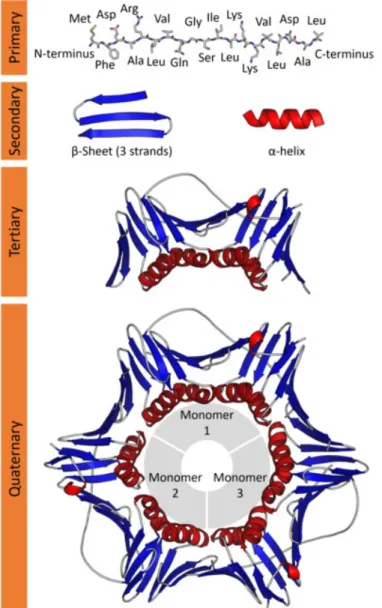
2.1 The four levels of the protein structure. . . 13

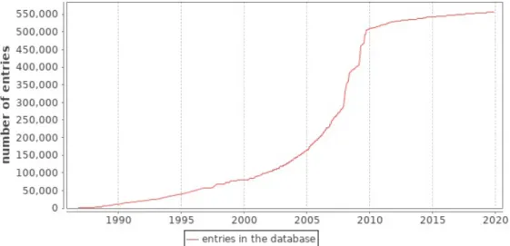
2.2 Number of entries of SwissProt database over time. . . 15

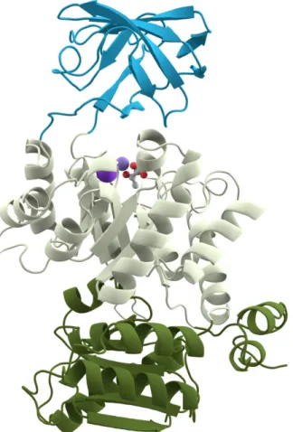
2.3 A visualization of the three domains of the protein Pyruvate kinase. 16 2.4 An overview of protein domains databases. . . 19

2.5 An illustration off the IRR prediction problem. . . 21

3.1 Standard supervised classification vs multiple instance classification 31 3.2 A classification problem of images into "beach" and "non-beach". 33 3.3 Illustrative example of an MIL problem where standard assumption should not be adopted. . . 34

3.4 Illustrative example using the IS paradigm. . . 36

3.5 Illustrative example using the BS paradigm: training and test. . . 37

3.6 Illustrative example using the ES paradigm: training and test. . . 38

3.7 Illustrative example showing the impact of treating the instances as non independently and identically distributed samples. . . 43

4.1 System overview of the naive approach for MIL in sequence data 51 4.2 System overview of the ABClass approach . . . 53

4.3 Accuracy results of the naive approach and ABClass . . . 64

4.4 Sensitivity results of the naive approach and ABClass . . . 64

4.5 Specificity results of the naive approach and ABClass. . . 66

5.1 Accuracy results of the naive approach, ABClass and ABSim. . . 77

5.2 Sensitivity results of the naive approach, ABClass and ABSim. . . 79

5.3 Specificity results of the naive approach, ABClass and ABSim. . . 79

6.1 Graphical representation of the InterProScan analysis of the protein P2 of the bacterium B7 . . . 85

List of Tables

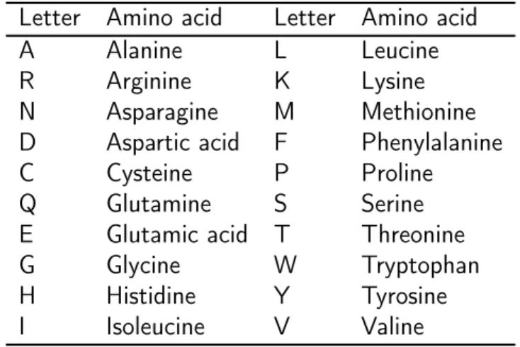
2.1 The 20 amino acids in a protein sequence. . . 11

4.1 IRRB and IRSB learning set. . . 59

4.2 Replication, repair and recombination proteins. . . 60

4.3 Sparsity of the attribute-value matrix used in the naive approach. 62

4.4 Number of extracted motifs for each set of orthologous protein sequences using a minimum motif length = 3. . . 63

4.5 Rate of successful classification models for each bacterium using ABClass approach and LOO evaluation method . . . 65

5.1 Experimental results of ABSim with LOO-based evaluation technique. 77

5.2 Number of successful predictions (for 8 runs) . . . 78

6.1 Tools related to protein signatures identification. . . 83

A.1 Number of protein sequences for each bacterium. . . I

A.2 Number of occurrences of each type of protein sequence in the positive and negative bags. . . II

Contents

1 Introduction 1

1.1 Context and motivations . . . 2

1.2 Contributions . . . 4

1.2.1 First axis: Motif-based MIL approach for sequence data with across-bag dependencies . . . 4

1.2.2 Second axis: Similarity-based MIL approach for sequence data with across-bag dependencies . . . 5

1.3 Outline . . . 5

I

Background and related works

7

2.1.1 Bioinformatics . . . 10

2.1.2 Biological data . . . 11

2.1.3 Proteins . . . 12

2.1.3.1 Protein structures . . . 12

2.1.3.2 Protein sequence data databases . . . 12

2.1.3.3 Protein signatures . . . 15

2.2 The bacterial ionizing radiation resistance problem . . . 20

2.3 Sequence Classification . . . 21

2.3.1 Definition of a sequence . . . 21

2.3.2 Sequence classification approaches in machine learning . . 22

2.4 Aligning biological sequences: basic notions . . . 23

2.4.1 What is the alignment of biological sequences . . . 23

2.4.1.1 Gaps . . . 24

2.4.1.2 Alignment scoring . . . 24

2.4.2.1 Dynamic programming based alignment . . . . 26

2.4.2.2 Heuristic based alignment . . . 26

2.5 Conclusion . . . 26

3 Multiple instance learning 29 3.1 Multiple instance learning . . . 30

3.1.1 Multiple instance learning VS standard supervised learning 30 3.1.2 Problem formulation . . . 30

3.1.3 Applications . . . 30

3.2 Background . . . 33

3.2.1 MIL assumptions . . . 33

3.2.2 Instance-level and bag-level learning . . . 35

3.3 An overview of MIL methods . . . 39

3.4 MIL for sequence data . . . 43

3.4.1 Related works using sequence data . . . 43

3.4.2 Problem Formulation . . . 45

3.4.3 Delimitation of the problem . . . 45

3.5 Conclusion . . . 46

II

Contributions

47

4.1.1 The algorithm . . . 50

4.1.2 Running example . . . 50

4.2 ABClass: Across-Bag sequences Classification approach . . . 53

4.2.1 The approach . . . 53

4.2.2 Running example . . . 54

4.3 Creating the bacterial IRR database . . . 57

4.4 Experimental study. . . 57

Contents ix

4.4.2 Experimental protocol . . . 58

4.4.3 Experimental results . . . 62

4.5 Conclusion . . . 67

5 Similarity-based MIL approach for sequence data with across-bag dependencies 69 5.1 ABSim: Across-Bag sequences Similarity approach . . . 70

5.1.1 The approach . . . 70

5.1.2 Aggregation methods: SMS and WAMS . . . 71

5.1.3 Running example . . . 74

5.2 Experimental study. . . 75

5.2.1 Experimental environment . . . 75

5.2.2 Results . . . 75

5.3 Conclusion . . . 80

6 Conclusion and prospects 81 6.1 Summary of the contributions . . . 82

6.1.1 ABClass: a motif-based MIL approach for sequence data with across-bag dependencies . . . 82

6.1.2 ABSim: a similarity-based MIL approach for sequence data with across-bag dependencies . . . 82

6.2 Future work and prospects . . . 83

6.2.1 Short-term perspective . . . 83

6.2.2 Long-term perspectives . . . 84

6.2.2.1 Multi-criteria learning . . . 84

6.2.2.2 Defining weights of the protein sequences . . . 84

6.2.2.3 Extend the dataset . . . 85

Bibliography 87

Appendix A Further details about the dataset I

Chapter 1

Introduction

Contents

1.1 Context and motivations . . . 2

1.2 Contributions . . . 4

1.2.1 First axis: Motif-based MIL approach for sequence data with across-bag dependencies . . . 4

1.2.2 Second axis: Similarity-based MIL approach for sequence data with across-bag dependencies . . . 5

1.3 Outline . . . 5 Goals

This chapter summarizes the contents and describes the plan of the thesis. First, we highlight the motivations of this work. Then, we state the addressed issues in this thesis.

1.1

Context and motivations

In a traditional setting of supervised learning task, the training set is composed of feature vectors (instances), where each feature vector has a label. In MIL task, we learn a classifier based on a training set of bags, where each bag contains multiple feature vectors and it is the bag that carries a label. We do not know the labels of the instances inside the bags.

This work was originally proposed to solve the problem of ionizing radiation resistance (IRR) prediction in bacteria [Zoghlami et al.,2019a,b,2018a,b] [Aridhi et al.,2016]. Ionizing-radiation-resistant bacteria (IRRB) are important in biotech-nology. In fact, they could be used for the treatment of radioactive wastes as well as the therapeutic industry [Brim et al., 2003] [Gabani and Singh, 2013]. Several in vitro works studied the causes of the high resistance of IRRB to ionizing radi-ation to determine peculiar features in their genomes and improve the treatment of radioactive wastes. Predicting if a bacterium belongs to IRRB using in vitro experiments is not an easy task, it requires a big effort and a time consuming lab work. In this thesis, we aim to use machine learning in order to perform the bacterial IRR prediction task . As far as we know, there is no bioinformatics tool that performs a such task in the literature. We propose an MIL formalization of the problem since each bacterium is represented by a set of protein sequences. Bacteria represent the bags and protein sequences represent the instances. In par-ticular, each protein sequence may differ from a bacterium to another, e.g., each bag contains the protein named Endonuclease III, but it is expressed differently from one bag to another: these are called orthologous proteins [Fang et al.,2010]. To learn the label of an unknown bacterium, comparing a random couple of sequences makes no sense, it is rather better to compare the protein sequences that have a functional relationship/dependency: the orthologous proteins. Hence, this work deals with the MIL problem that has the following three criteria:

• The instances inside the bags are sequences: to deal with sequences, we have to deal with data representation. A widely used technique to rep-resent MIL sequence data is to apply a preprocessing step which extracts features/motifs to represent the sequences [Sutskever et al., 2014] [Lesh

1.1. Context and motivations 3 et al., 1999] [She et al., 2003]. Other works keep data in their original format and use sequence comparison techniques such as defining a distance function to measure the similarity between pairs of sequences [Aridhi et al.,

2016] [Saigo et al., 2004] [Xing et al.,2010].

• All the instances inside a bag contribute to define the bag’s label: the standard MIL assumption states that every positive bag contains at least one positive instance while in every negative bag all of the instances are negative. Some methods following this assumption try to identify positive instances which are relevant to learn the label of a bag [Faria et al.,2017] [Li et al., 2014]. However, the collective assumption [Amores, 2013] considers that all the instances contribute to the bag’ s label. This suits the problem of bacterial IRR prediction since all the protein sequences have to contribute to the final decision.

• The instances may have dependencies across the bags: one ma-jor assumption of most existing MIL methods is that each bag contains a set of instances that are independently distributed. Nevertheless, in many applications, the dependencies between instances naturally exist and if in-corporated in the classification process, they can potentially improve the prediction performance significantly [Zhang et al., 2011]. Many real world applications such as bioinformatics, web mining, and text mining have to deal with sequence data. When the tackled problem can be formulated as an MIL problem, each instance of each bag may have structural and/or temporal relation with other instances in other bags. This is the case of the IRR prediction problem in which the bags contain orthologous protein sequences.

Considering this issue, the problem we want to solve in this work is the MIL problem in sequence data that have dependencies between instances of different bags.

1.2

Contributions

In this work, we present two novel MIL approaches for sequence data classifica-tion named ABClass ( which stands for Across Bag sequences Classificaclassifica-tion) and ABSim ( which stands for Across Bag sequences Similarity). ABClass is a motif-based approach while ABSim uses a similarity measure between related sequences. We applied both approaches to solve the problem of IRR prediction. The experimental results were satisfactory.

1.2.1

First axis: Motif-based MIL approach for sequence

data with across-bag dependencies

As a first contribution, we propose a motif-based approach, named ABClass, which takes into account the across-bag relations between the sequences of different bags in the classification process. In a motif-based classification for sequential data, a sequence is transformed into a feature/motif vector. The feature extraction step is very important in the classification process. Many parameters have an impact in the classification results such as the motifs frequency and length, and the matching type between motifs. Feature-based approaches are widely adopted for genomic sequence classification. In ABClass, a preprocessing step is performed in order to extract motifs from each set of related sequences. These motifs are then used as attributes to construct a vector representation for each set of sequences. In order to compute partial prediction results, a discriminative classifier is applied to each sequence of the unknown bag and its correspondent related sequences in the learning dataset. Finally, an aggregation method is applied to generate the final result.

We created a multiple instance dataset composed of real sequence data used to test the approach. It consists of a set of bacteria where each bacterium is represented using a set of primary structures of proteins implicated in basal DNA repair in IRRB. Bacteria represent the bags and protein sequences represent the instances. The used across-bag relation is the orthology. Orthologous proteins are assumed to have the same biological functions in different species. The dataset is

1.3. Outline 5 publicly available athttp://homepages.loria.fr/SAridhi/software/MIL/ .

1.2.2

Second axis: Similarity-based MIL approach for

se-quence data with across-bag dependencies

As a second contribution, we propose the ABSim algorithm. It does not use motifs to represent data and no encoding step is needed. We use a similarity measure between each sequence of the unknown bag and the corresponding sequences in the learning bags in order to create a similarity score matrix. An aggregation method is applied and the unknown bag is labeled according to the bag that presents more similar sequences. We define two aggregation methods: Sum of Maximum Scores (SMS) and Weighted Average of Maximum Scores (WAMS). In the experimental study, we used the local alignment score to measure the similarity between two protein sequences.

1.3

Outline

The remainder of this document is organized as follows. Chapter 2 presents the bioinformatics field and gives a background about the processed data and the alignment of biological sequences. It also provides a description of the bacterial IRR prediction problem. Chapter 3 provides a background about MIL fundamen-tal notions and gives an overview of some related works in MIL. It also gives a formalization of the problem of MIL in sequence data. In Chapter 4, we present an MIL naive approach for sequence data followed by a description of the AB-Class algorithm. We provide a simple use case that serves as a running example throughout the chapters 4 and 5. Then we describe our experimental environment and we discuss the obtained results. Chapter 5 describes the ABSim approach and the two proposed aggregation methods. Concluding points and a presentation of future work make the body of Chapter 6.

Part I

Chapter 2

Bioinformatics and Sequence

classification

Contents

2.1.3.2 Protein sequence data databases . . . 12

2.1.3.3 Protein signatures . . . 15

2.2 The bacterial ionizing radiation resistance problem . . . 20

2.3 Sequence Classification . . . 21

2.3.1 Definition of a sequence . . . 21

2.3.2 Sequence classification approaches in machine learning. . . 22

2.4 Aligning biological sequences: basic notions . . . 23

2.4.1 What is the alignment of biological sequences. . . 23

2.4.1.1 Gaps . . . 24

2.4.1.2 Alignment scoring . . . 24

2.4.2 Global alignment and local alignment . . . 25

2.4.2.1 Dynamic programming based alignment . . . 26

2.5 Conclusion . . . 26 Goals In this chapter, we will present basic notions of a main search field in this thesis: bioinformatics. We present mainly the specificity of the biological data and we introduce the investigated IRR prediction problem. We present also the particularity of sequence classification in the data mining field and we focused on the alignment of biological sequences.

2.1

Bioinformatics background

2.1.1

Bioinformatics

Bioinformatics in an interdisciplinary field which can be simply defined by the use of computer science to deal with biological data. Developing software programs to produce meaningful biological information involves the use of algorithms from dif-ferent disciplines such as data mining, graph theory, statistics, artificial intelligence and image processing.

The aims of bioinformatics involve mainely the collection and storage of data in a way that allows to access them efficiently and the development of algorithms and tools that deal with the analysis, prediction and interpretation of the data.

To date, the genomic databases indicate the presence of thousands of genome projects. It is not feasible to analyze the amount of collected data manually without using tools that make the task easier. It is impossible to experimentally annotate every biological molecule identified by sequencing projects. Bioinformat-ics has then evolved in the past few years in order to provide software applications that need minutes or even seconds to accomplish tasks that used to require a big effort and weeks of lab work. Computational approaches could be used to provide initial prediction results related to the function of a biological molecule and help to predict the usefullness of an experimental study scenario. Examples of bioinfor-matics research fields include the sequencing of genomes, the 3-D visualisation of molecules, the construction of evolutionary trees, the analyses of protein functions and the ionizing radiation resistance prediction (See Section 2.2).

2.1. Bioinformatics background 11 Table 2.1: The 20 amino acids in a protein sequence.

Letter Amino acid Letter Amino acid

A Alanine L Leucine

R Arginine K Lysine

N Asparagine M Methionine

D Aspartic acid F Phenylalanine

C Cysteine P Proline

Q Glutamine S Serine

E Glutamic acid T Threonine

G Glycine W Tryptophan

H Histidine Y Tyrosine

I Isoleucine V Valine

2.1.2

Biological data

Mainly, bioinformatics deals with three biological macromolecules named protein, DNA and RNA. The last two macromolecules are called nucleic acids.

• Proteins They are macromolecules responsible of a variety of functions within organisms such as DNA replication, and transporting molecules from one location to another. They are complex chains of molecules known as amino acids so they can be viewed as strings of an alphabet of the 20 amino acids provided in Table 2.1.

• Nucleic acids. Nucleic acids include DNA and RNA macromolecules. – DNA Deoxyribonucleic acid (shortly DNA) is known to be the molecule

that carries the genetic instructions of organisms. It has a double helical twisted structure. Each side is made of four bases which are represented by the four letters A (adenine), C (cytosine), G (guanine) and T (thymine). A DNA could then be represented by a sequence of the alphabet {A,C, G, T }.

– RNA Ribonucleic acid (shortly RNA) is a molecule very similar to DNA but has some chemical differences. It play various roles in coding, decoding, and expression of genes. The four bases are the same as in

DNA with thymine (T) replaced by uracyl (U). Then, an RNA molecule could be represented by a sequence of the alphabet {A,C, G,U}.

2.1.3

Proteins

2.1.3.1 Protein structures

There are four levels of protein structures as described in Figure 2.1.

• Primary structure: A primary structure represents a protein as a sequence of amino acids which attach to each other in long chains. The terms protein or polypeptide refers to sequences longer than 50 amino acids while sequences with fewer amino acids are called peptides.

• Secondary structure: The chain of amino acids can fold to form a three-dimensional structure. Two main types of secondary structure are the α-helixes and β -sheets.

• Tertiary structure: The secondary structures are folded to form the over-all shape of a protein, also known as the protein 3-D structure or the tertiary structure.

• Quaternary structure: Several proteins are composed of more than one se-quence of amino acids. The combination of these sese-quences conform the quaternary structure.

2.1.3.2 Protein sequence data databases

With the evolution of sequencing technologies, the amount of biological sequence data has exponentially increased. Some publicly available databases offer to users the possibility to search and download protein sequence data.

• GOLD database The Genomes OnLine Database (GOLD) [Mukherjee et al., 2016] provides a comprehensive information regarding genome and metagenome sequencing projects with their associated metadata. Data are

2.1. Bioinformatics background 13

Figure 2.1: The four levels of the protein structure 1.

imported from three main sources: (1) projects deposited by users which are regularly monitored for data accuracy and consistency, (2) projects imported from public resources like BioProject database [Federhen et al.,

1

https://en.wikipedia.org/wiki/File:Protein_structure_(full).png, Novem-ber 2019.

2014] and (3) projects sequenced at the Joint Genome Institute (JGI) 2. The latest publication reported 97 212 Sequencing Projects. GOLD is available at https://gold.jgi.doe.gov/.

• UniProt The Universal Protein resource (UniProt) is a biological reposi-tory of protein sequences and their functional information [Apweiler et al.,

2004]. It contains four databases: Swiss-Prot and TrEMBL which are sub-parts of UniProtKB, UniParc and UniRef.

SwissProt contains non-redundant, manually annotated protein sequences [Boutet et al., 2016]. In order to perform the annotations, information ex-tracted from biological literature are combined with computational analysis evaluated by biocurator. The goal is to provide relevant known informa-tion related to proteins available in the database. Figure 2.2 shows the increasing size of SwissProt database over thirty years. The amount of available protein sequences was doubled during three years from 2007 to 2010. TrEMBL is a database that contains automatically annotated pro-tein sequences [Gane et al., 2014]. In fact, the large amount of data gen-erated by genome projects could not be manually analysed and annotated according to the process of UniProtKB/SwissProt. Thus, data are auto-matically processed and added to the TrEMBL database. UniParc (for UniProt Archive) [Leinonen et al.,2004] contains non-redundant protein se-quences from the main publicly available databases. UniRef (for UniProt Reference Clusters) [Suzek et al.,2007] contains clustered protein sequences from SwissProt, TrEMBL and selected UniParc entries.

• GenBank and RefSeq The National Centre for Biotechnology Infor-mation (NCBI) 3

hosts two sequence databases named GenBank [ Ben-son et al., 2012] and RefSeq [Pruitt et al., 2011]. GenBank and RefSeq provide an annotated collection of publicly available nucleotide and pro-tein sequences, while UniProt contains only propro-tein sequence data, Un-2

https://jgi.doe.gov

3

2.1. Bioinformatics background 15 like GenBank sequences, RefSeq ones are non-redundant, curated and lim-ited to some organisms for which sufficient data are available. GenBank contains sequences for any submitted organism. Refseq is available at

https://www.ncbi.nlm.nih.gov/refseq/ and GenBank is available at

https://www.ncbi.nlm.nih.gov/genbank/.

Figure 2.2: Number of entries of SwissProt database over time 4 .

2.1.3.3 Protein signatures

Protein signatures consist of models which describe protein families, domains or sites. A protein family is a group of proteins that share the same evolutionary origin. Proteins in a same family have similar sequences/structures and biological functions. Families are usually hierarchically organized. A domain is a part of a protein which is able to evolve, function, and exist independently of the rest of the protein sequence/structure. From sequence perspective, a protein domain is a subsequence of amino acids. Domains vary in length from about 25 amino acids to 500 amino acids. They also vary in biological functions. The average size of protein domains is 150 amino acids. The concept of protein domains

4

and families are applicable to both sequences and structural proteins. Several proteins are multi-domain. Figure 2.3 shows a visualization of the three domains of the protein Pyruvate kinase, each domain has a different color. The ordered arrangement of domains in a protein, called the protein domain organization or the protein domain architecture, is important to maintain the function and the structure of the protein.

Figure 2.3: A visualization of the three domains of the protein Pyruvate kinase6 . Signature could be simple such as patterns or more complex such as Hidden Markov Models (HMMs). Signature methods are divided into patterns, profiles, fingerprints and HMMs. Conserved subsequences, also known as motifs, are

6

https://commons.wikimedia.org/wiki/File:Pyruvate_kinase_protein_domains. png, November 2019

2.1. Bioinformatics background 17 extracted and then used to build regular expressions that serve as patterns. Profiles are computed by converting multiple sequence alignments into position-specific scoring systems (PSSMs), i.e., assigning a score to amino acids at each position according to the frequency with which they occur in the alignment. Fingerprints are created using multiple profiles generated using multiple alignment techniques. The main advantage of fingerprints is in identifying the differences in protein sequences at four levels of clan, superfamily, family and subfamily which helps to make a more accurate functional predictions for unknown sequences. HMMs are statistical models that, like profiles, convert multiple sequence alignments into PSSMs and represent amino acid insertions and deletions. Its can model the entire alignment, including divergent regions.

Figure2.4 shows a list of well known protein domain databases grouped based on the used protein signatures. Domain databases are described below.

• Prosite provides entries that describe protein domains and families, and related patterns and profiles used to identify them. It contains documen-tation about signatures and the structure and function of proteins. Fig-ure 2.4 differentiates between Prosite entries based on patterns (in or-ange) and those based on profiles (in green). The database is available athttp://prosite.expasy.org/.

• Prints is a database of fingerprints [Attwood et al.,2003] which contains an annotation list for protein families and a diagnostic tool for newly discovered protein sequences. The database is accessible at http://www.bioinf. man.ac.uk/dbbrowser/PRINTS/.

• CDD [Marchler-Bauer et al., 2005] [Marchler-Bauer et al., 2014] is the Conserved Domain Database for the functional annotation of proteins. It includes manually curated domain models from NCBI (National Cen-ter for Biotechnology Information in ) and other domain models im-ported from a set of external databases such as Pfam, and TIGR-FAMs. In order to generate NCBI-curated domains, 3D-structure in-formation is used to characterize domains and relationship between into

sequences and related structure and function. CDD is accessible at http://www.ncbi.nlm.nih.gov/Structure/cdd/cdd.shtml.

• Pfam is a database of protein domains and families represented by multiple sequence alignments and hidden Markov models (HMMs) [Bateman et al.,

2004] [Finn et al., 2015]. It has a large coverage of proteins and a real-istic way of naming domains. It provides two subsets data depending on the quality of the families: Pfam-A and Pfam-B. Pfam-A provides man-ually curated families with high quality alignments and well-characterized protein domains. Pfam-B contains a lower quality data where families are automatically generated.

• TIGRFAMs [Haft et al., 2003] [Haft et al., 2012] is a database of pro-tein families that supports manual and automated curated genome an-notation. It includes multiple sequence alignments and a corresponding HMM generated from the alignment. If the score of a sequence ex-ceeds a defined threshold of a given TIGRFAMs HMM, the protein se-quence is assigned to the related protein family. TIGRFAMs is available athttp://www.jcvi.org/cgi-bin/tigrfams/index.cgi.

• Panther ( for Protein ANalysis THrough Evolutionary Relationships) [Thomas et al., 2003] [Mi et al., 2016] is a large collection of protein fami-lies manually subdivided into functionally related subfamifami-lies. A phylogenetic tree is built for each family and could be used in order to classify an un-characterized protein sequence. Each node in the tree is annotated with heritable attributes that are propagated to a decedent node. A protein is then annotated according to its ancestor in the phylogenetic tree. Panther database is available viahttp://pantherdb.org/.

• SMART (Simple Modular Architecture Research Tool) [Schultz et al.,1998] [Letunic et al.,2011] is a database that provides the identification of domains and the analysis of their architectures. It uses HMMs built from multiple sequence alignments in order to identify protein domains. SMART data was used to create the CDD database.

2.1. Bioinformatics background 19

Figure 2.4: An overview of protein domains databases [Alborzi, 2018].

• CATH [Orengo et al., 1997] [Pearl et al., 2003] is a database of curated classification of protein domain structures [Orengo et al., 1997, Pearl et al., 2003]. In order to perform this classification, a combination of multiple procedures is used including literature review, expert analysis, computational algorithms and statistical analysis. It shares many features with the SCOP resource, however they may differ greatly in detailed classification. CATH database is available athttp://www.cathdb.info/.

• SCOP (Structural Classification of Proteins) database [Murzin et al., 1995] is a classification of structural domains of the proteins based on their evolutionary and structural relationships. The goal is to provide a com-prehensive and detailed description of the relationships between all pro-teins having known 3D structures. SCOP database is available at http: //scop.mrc-lmb.cam.ac.uk/scop/. It stopped updating in 2010 and a successor named SCOP2 [Andreeva et al.,2013] has been proposed. SCOP2 is available athttp://scop2.mrc-lmb.cam.ac.uk/.

In-terPro database [Apweiler et al., 2001] [Finn et al., 2016]. In fact, InterPro is a composite database combining the information of many databases of protein domains. The goal is to rationalise protein sequence analysis by combining infor-mation from different resources in a consistent manner, removing redundancy, and adding rich annotation about the proteins and their signatures. Features found in known proteins are applied to unknown ones (such as new sequenced proteins) in order to characterise their functions. It contains signatures and the proteins that they significantly match. InterproScan is a tool used to search a query against the diverse databases of protein domains, motifs, signatures and families. The disadvantage is the runtime since the Interproscan webservice can be very slow if we need to analyse thousands of proteins. A solution is to download and install the whole suite locally.

2.2

The bacterial ionizing radiation resistance

problem

Bacteria are small single-cell organisms. Most bacteria are helpful for mankind, but some are harmful. Few species cause disease. In particular, ionizing-radiation-resistant bacteria (IRRB) are important in biotechnology. They could be used for the treatment of mixed radioactive wastes by developing a strain to detoxify both mercury and toluene [Brim et al., 2000]. These organisms are also being engineered for in situ bioremediation of radioactive wastes[Brim et al., 2003]. In [Gabani and Singh, 2013], the authors discuss the potential uses of radiation-resistant extremophiles (e.g. micro-organisms with the ability to survive in extreme environmental conditions) in biotechnology and the therapeutic industry.

Several in vitro and in silico works studied the causes of the high resistance of IRRB to ionizing radiation to determine peculiar features in their genomes and improve the treatment of radioactive wastes. However, limited computational works are provided for the prediction of bacterial IRR [Aridhi et al.,2016] [Sghaier et al., 2008][Makarova et al., 2007]. In this thesis, we aim to develop a machine learning algorithm which predicts whether an unlabelled bacterium belongs to

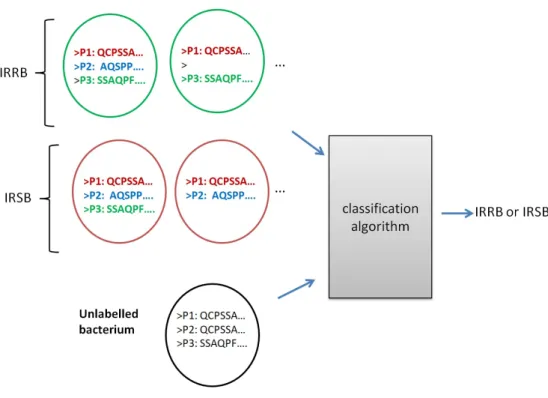
2.3. Sequence Classification 21 IRRB or IRSB. Each bacterium is represented using a set of protein sequences implicated in basal DNA repair (see Figure 2.5).

Figure 2.5: An illustration off the IRR prediction problem.

2.3

Sequence Classification

2.3.1

Definition of a sequence

A sequence is an ordered list of events. An event can be represented as a symbolic value, a numerical value, a vector of values or a complex data type [Xing et al., 2010]. There are many types of sequences including symbolic sequences, simple time series and multivariate time series [Xing et al., 2010]. In our work, we are interested in symbolic sequences since the protein sequences are described

using symbols (amino acids). We denote Σ an alphabet defined as a finite set of characters or symbols. A simple symbolic sequence is defined as an ordered list of symbols from Σ.

2.3.2

Sequence classification approaches in machine

learning

Existing sequence classification approaches can be divided into three large cate-gories [Xing et al.,2010]: feature-based classification, distance-based classification and model-based classification.

In feature-based classification, a sequence is transformed into a feature vector. This representation scheme could lead to very high-dimensional feature spaces. The feature extraction step is very important since it would impact the classifi-cation results. This step should deal with many parameters such as the criteria used for selecting features (e.g. frequency and length) and the matching type (i.e. exact or inexact with gaps). After adapting the input data format, a con-ventional classification method is applied. Feature-based approaches are widely adopted for genomic sequence classification [Blekas et al.,2005] [She et al.,2003] [Chuzhanova et al., 1998].

In distance-based classification, a similarity function should be defined to mea-sure the similarity between a pair of sequences. Then an existing classification method could be used such as the Support Vector Machine (SVM) or the K-Nearest Neighbors (KNN) algorithm. The similarity function determines the qual-ity of the classification significantly. In bioinformatics, alignment based distances are popularly adopted to deal with sequences such as protein sequences and DNA sequences. Section 2.4 provides an overview on biological sequences alignment.

Model-based classification methods define a classification model based on the probability distribution of the sequences over the different classes. This model is then used to classify unknown sequences. Naive Bayes is a simple model-based classifier that makes the assumption that the features of the sequences are independent. In [Cheng et al., 2005], the authors apply Decision Tree and Naïve Bayes classifiers on a protein classification problem. Markov Model and

2.4. Aligning biological sequences: basic notions 23 Hidden Markov Model (HMM) could be used in order to model the dependencies among sequences. In [Yakhnenko et al.,2005], a k-order Markov model is used to classify protein sequences and text data. HMM and alignment scores are used in [Srivastava et al., 2007] in order to make a genomic sequences classification. A protocol named HMM-ModE is defined in order to generate family specific HMMs. Hierarchical clustering is also commonly used in genomic sequences/organisms classification [Ni et al., 2018] [Pagnuco et al., 2017] [Lukjancenko et al., 2010]. It groups the samples into groups called clusters. In the clustering process, inter-cluster distances should be maximized and intra-inter-cluster distances should be min-imized. Hierarchical clustering produces a nested series of clusters which may be represented in a tree structure, called a dendrogram, which may facilitate the interpretation of the classification results. In order to create the clusters, the genomic sequences are compared. Although the sequence alignment score is com-monly used to make the comparison, some hierarchical clustering algorithms use alignment-free comparison methods [Ni et al.,2018] [Wei et al.,2012].

2.4

Aligning biological sequences:

basic

no-tions

2.4.1

What is the alignment of biological sequences

The sequence alignment problem is one of the cornerstones of computational bi-ology. Sequence alignment is a way of arranging sequences in order to identify regions of similarity. This similarity could provide a structural, functional or evo-lutionary significance. The majority of biological sequence comparison methods rely on first aligning sequences and computing a score for the alignment [Vinga and Almeida, 2003].

As stated, the goal is to line up two (or more) sequences in order to maximise their degree of similarity. Identical bases are matched In the case of DNA and RNA. For proteins, amino acids are matched if they are identical. An amino acid could be replaced by another one on the basis of a substitution matrix.

Some genomic sequences comparison problems are not simply resolved using one or two alignment tool. In [Gracy and Argos, 1998], local similarity search is coupled to multiple sequence alignment in order to classify an entire protein sequence database. Additional contextual information could be integrated in or-der to improve the genomic sequences comparison. Domain co-occurrence is a powerful feature of proteins which can be used in this context [Menichelli et al.,

2018].

2.4.1.1 Gaps

When the sequences do not align well with each other, a gap could be inserted into any of the sequences by pushing a letter one index. The goal is to obtain a better alignment. A gap is marked by the symbol ´- ´. The biological interpretation of using a gap is that a mutation (a deletion or an insertion) occurred during the evolution of a sequence.

Example of an alignment using the two sequences TACCAGT and CCCG-TAA

No gaps Gaps

T A C C A G T T A C C A G T − −

C C C G T A A C − C C − G T A A

We note that other alignments are possible, an option is listed below.

T A C C A G T − −

− C C C G T A A −

2.4.1.2 Alignment scoring

As different alignments are possible, we can use a scoring function in order to select the best alignment. Gap penalty functions are used in order to compute an alignment score based on the number and length of gaps. The idea is that inserting too many gaps can lead to a meaningless alignment, so we need to minimize the

2.4. Aligning biological sequences: basic notions 25 number of gaps. Some gap penalty functions are listed below.

• Constant gap penalty It is a simple scoring function. A fixed negative cost is assigned to every gap, regardless of its length.

• Linear gap penalty A fixed negative score is assigned to every inserted or deleted symbol. The penalty is then directly proportional to the length of the gap.

• Affine gap penalty. It is a widely used scoring function. Different scores are assigned to the extension of a current gap and the starting of a new one. If we perform an alignment of protein sequences, substitution matrices could be used in the scoring alignment instead of using fixed scores. In fact, some amino acids have similar structures and can be substituted in nature. Mutations of amino acids are quantified in the substitution matrices Two well-known matrices are PAM [Dayhoff et al., 1978] and BLOSUM [Henikoff and Henikoff,1992].

2.4.2

Global alignment and local alignment

In pairwise alignment, only two sequences are involved in the alignment process, otherwise, it is a multiple sequence alignment. Alignment technics could be divided into two types based on the completeness:

• global alignment which attempts to match the sequences to each other from end to end. It is suitable for similar and equal length sequences. • local alignment which searches for highly similar regions of the two

se-quences. It is more suitable for sequences which are partially similar and/or have different length. It is then useful for comparing sequences that share a common conserved pattern (motif) but differ elsewhere.

Several sequence alignment approaches have been proposed. Some algorithms use dynamic programming and provide optimal alignments such as the Needleman-Wunsch algorithm [Needleman and Wunsch, 1970] and The Smith-Waterman [Waterman, 1981] algorithm. Other alignment methods are based on heuristics such as BLAST, the widely used alignment tool in bioinformatics.

2.4.2.1 Dynamic programming based alignment

Dynamic programming is originally used in the field of mathematical optimization [Sniedovich, 2010]. In computer science, dynamic programming is the approach based on dividing a problem into smaller subproblems. Each of the subproblems is divided further into subproblems until some basic case is reached. Needleman-Wunsch algorithm [Needleman and Wunsch, 1970] and Smith-Waterman algo-rithm are based on Dynamic Programming. The first one is a classical global alignment algorithm while the second one performs a local alignment. Both ap-proaches produce an optimal alignment based on a scoring matrix. A gap penalty could be used during the alignment process.

2.4.2.2 Heuristic based alignment

Heuristic approaches are much faster than dynamic programming ones, but they may overlook optimal alignments. They are widely used in large-scale database searches. BLAST [Altschul et al.,1990] (stands for Basic Local Alignment Search Tool) is a well-known alignment tool. It performs local alignment, i.e., it does not enforce the alignments on full length to measure the similarity between two sequences. BLAST requires a query sequence to search for, and a target sequence to search against or a sequence database containing multiple target sequences. The algorithm splits the query sequence into small subsequences and scans the database for word matches. All matches are then extended in both directions as far as possible in order to seek high-scoring alignments. Many extensions of BLAST have been proposed such as PSI-BLAST [Altschul et al.,1997] and BLAT [Kent, 2002] [Bhagwat et al.,2012]. The main idea of BLAST-like methods is to identify short common subsequences between the sequences, and then expand the matching regions.

2.5

Conclusion

In this chapter, we introduced basic notions the bioinformatics research field. We presented the biologial data sequences and we introduced the bacterial IRR

2.5. Conclusion 27 prediction problem that we aim to investigate in this work. We focused on the alignment of biological sequences.

Chapter 3

Multiple instance learning

Contents

3.1 Multiple instance learning . . . 30

3.1.1 Multiple instance learning VS standard supervised learning. 30

3.1.2 Problem formulation . . . 30

3.1.3 Applications . . . 30

3.2 Background . . . 33

3.2.1 MIL assumptions . . . 33

3.2.2 Instance-level and bag-level learning . . . 35

3.3 An overview of MIL methods . . . 39

3.4 MIL for sequence data . . . 43

3.4.1 Related works using sequence data . . . 43

3.4.2 Problem Formulation . . . 45

3.4.3 Delimitation of the problem . . . 45

3.5 Conclusion . . . 46 Goals This chapter introduces the MIL and its paradigms. It is mainly dedi-cated to present, in a simplified way, the basic notions related to MIL. We mainly focus on presenting MIL paradigms and describing some approaches.

3.1

Multiple instance learning

3.1.1

Multiple instance learning VS standard supervised

learning

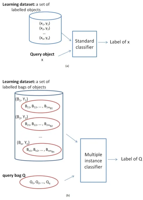
The standard supervised learning task deals with data that consist of a set of objects/examples, where each object is associated with a label. The learning dataset contains n labeled object DB = {(xi, yi), i = 1, . . . , n} where xi is a seen

example and yi is the label that indicates the category that the object xi belongs

to (see Figure 3.1) . An MIL task deals with data that consist of a set of n bags where each bag is an unordered set of examples (see Figure 3.1). In an MIL context, each example is called an instance. MIL can be seen as a variant of supervised learning. However, labels are assigned to bags rather than individual instances. This category of learning is considered as weakly supervised since we do not know the label of each instance inside the bag, and only bags carry the labels. In this thesis, we only consider two-class classification problems, so the label of each bag is either 1 for a positive bag or -1 for a negative one.

3.1.2

Problem formulation

Let DB be a learning database that contains a set of n labeled bags DB = {(Bi,Yi), i = 1, 2 . . . , n} where Yi= {−1, 1} is the label of the bag Bi. Instances

in Bi are denoted by Bi j. Formally Bi= {Bi j, j = 1, 2 . . . , mBi}, where mBi is the

total number of instances in the bag Bi. We note that the bags do not contain

the same number of instances. The goal is to learn a multiple instance classifier from DB. Given a query bag Q = {Qk, k = 1, 2 . . . , q}, where q is the total number

of instances in Q, the classifier should use data in this bag and in each bag of DB in order to predict the label of Q.

3.1.3

Applications

MIL has many real word applications including the drug activity problem, the image categorization and the text categorization.

3.1. Multiple instance learning 31

Figure 3.1: Standard supervised classification (a) vs multiple instance classification (b).

• Drug activity The original application for MIL is the drug activity predic-tion problem described in [Dietterich et al.,1997]. It deals with the first MI

dataset known as the musk dataset which contains molecules occurring in different conformations. One of the conformations determines if a molecule belongs to either "musk" class or "non-musk" one. In fact, if a molecule is able to bind strongly to a binding site on the target molecule, it is classi-fied as a good drug. The molecule is a bag and its conformations are the instances inside this bag. The musky smell is the positive label. We do not know which conformations bind well on a target molecule so we have no idea which instances are positive.

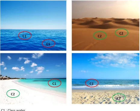
• Image categorization When applying MIL to the image categorization problem, an image is considered as a bag and its subimages are considered as instances that conform the bag. A processed image is then affiliated into one class or another. Several works use MIL in image categorization. In [Maron and Ratan, 1998], authors treat the natural scene images as bags. A bag is classified as a scene of waterfall if at least one of its subimages is a waterfall. In [Andrews et al., 2003] , the positive images show an animal (a fox, a tiger or an elephant), the negative images are selected randomly from other classes (the classes represent more than these three animals). An other image categorization problem defines a bag as an eye fundus image and an instance as a patch [Kandemir and Hamprecht, 2015]. The goal is to predict whether an image is of a subject with diabetes (positive) or a healthy subject (negative).

• Text categorization When dealing with a document categorization prob-lem using an MIL setting, a document is considered as a bag, and its para-graphes are considered as instances. In [Ray and Craven, 2005], authors study a problem of biomedical text categorization. The goal was to predict whether a text should be annotated as relevant for a particular protein. A bag is a biomedical text and instances are paragraphs in the document. The newsgroup dataset [Zhou et al., 2009] is a popular text categorization MI dataset. The goal is to categorize collections of posts from different news-groups corpus. A bag is a collection of posts (instances). A positive bag for a category contains 3% of posts about a topic while negative bags contain

3.2. Background 33 only posts about other topics.

3.2

Background

3.2.1

MIL assumptions

The standard MIL assumption states that a bag is positive if and only if one or more of its instances are positive while in every negative bag all of the instances are negative. This assumption is used in many MIL problems such as traditional problem of musk drug activity described in Section 3.1.3. A molecule is classified according to its conformations. If one on more conformations bind well to the target site, then the molecule belongs to the positive class.

Figure 3.2: A classification problem of images into "beach" (bottom) and "non-beach" (top).

3.2. Background 35 have the standard MI assumption witch is a special case of the presence-based MI assumption.

• The threshold-based MI Assumption requires that, in order to consider a bag as positive, a certain number of instances in the bag have to belong to each of the required concepts.

• The count-based MI Assumption is close to the previous assumption but it requires that a maximum and a minimum number of instances have to belong to each of the required concepts.

• The collective assumption supposes that all instances in a bag contribute equally to the bag’s label [Foulds and Frank, 2010]. All instances are con-sidered in the learning process.

• The weighted collective MI assumption is an extension of the previous as-sumption that uses different weights for each instance.

We note that many MI approaches do not use the standard assumption but it is not always stated which new assumption is adopted instead.

3.2.2

Instance-level and bag-level learning

MIL methods could be categorized according to how the information contained in the MIL data is exploited. In [Amores,2013], the author proposed to differentiate between the Instance-Space (IS) paradigm and the Bag-Space (BS) paradigm. A third category of MIL approaches based on the Embedded-Space (ES) paradigm was proposed. In this section, a lower-case notation will be adopted to refer instances (x) and instance-level classifiers (f), an upper-case notation is used to denote bags (X) and bag-level classifiers (F).

• Instance level The IS paradigm is based on local instance-level infor-mation since we consider the characteristics of individual instances in the learning process without looking at more global characteristics of the whole bag. Figure 3.4 illustrates the IS paradigm. A discriminative instance level

classifier f (x) is trained on the instances in order to separate instances of positive bags ( f (x) = 1) from instances in negative bags ( f (x) = 0). A bag level classifier F(X) is then obtained by applying an aggregation on instance level results. Diverse Density and MISVM are two examples of algorithms which use the IS paradigm (see Section 3.3).

Figure 3.4: Illustrative example using the IS paradigm [Amores, 2013].

• Bag level In the BS paradigm each bag is treated as a whole entity. Instead of aggregating instance-level decisions, a global bag-level information is used to make the discriminative decision. Figure 3.5 provides an illustrative ex-ample using the BS paradigm. In the training step, a distance function is defined to compare two bags. Then, a learning algorithm is applied to create a model. In order to predict its label, a new bag is compared to other bags of the training set using the bag level distance function. A classifier F uses the computed distances, the model and the learned parameters Θ to make the prediction. Citation-Knn is an example of algorithms which use the BS paradigm.

• Embedded level In the ES paradigm, the relevant information about each bag is summarized in a single feature vector. The difference between BS and ES paradigms lies in the way this bag-level information is extracted: it is done implicitly in the BS paradigm and explicitly in the ES one through the definition of a mapping function. An illustration of using ES learning is

3.2. Background 37

Figure 3.5: Illustrative example using the BS paradigm [Amores, 2013]: training (a) and test (b)

provided by the Figure 3.6. In the training step, the original training space is mapped to a vectorial embedded space by defining a mapping function M which associates a feature vector to each bag. A standard discriminant classifier G is then learned. In order to predict the class of a new bag X, the mapping M is used to generate the correspondent feature vector ~v. The

bag classifier F(x) is the obtained using the discriminant classifier G and the new vector v. It can be expressed as F(X) = G(~v). A simple algorithm that uses the ES paradigm is SimpleMI described is Section 3.3.

Figure 3.6: Illustrative example using the ES paradigm [Amores, 2013]: training (a) and test (b)

3.3. An overview of MIL methods 39

3.3

An overview of MIL methods

The original work that introduces the MIL problem proposes the axis-parallel hyper-rectangle (APR) approach [Dietterich et al., 1997]. It tries to identify an hyper-rectangle that includes at least one instance of every positive bag and does not in-clude any instances from negative bags. Many MIL approaches are then proposed. Diverse Density (DD) [Maron and Lozano-Pérez,1998] is one of the popular MIL algorithms. It was proposed as a general framework for solving MIL problems. Several MIL approaches have been proposed. Some algorithms deal with the MIL problem directly in either instance level such as mi-SVM [Andrews et al., 2003] and MILKDE [Faria et al., 2017] or in bag level such as MI-SVM mi-SVM [ An-drews et al.,2003] and MIGraph [Zhou et al.,2009]. Other algorithms try to shift the MIL problems into instance space via embedding such as MILDE [Amores,

2015], Submil [Yuan et al.,2016] and miVLAD [Wei et al.,2016]. Several regular supervised classifiers are extended to work in the MIL setting such as MI-SVM and Citation-kNN which extend respectively the SVM and the k-nearest neigh-bours approaches. Methods which are based on instance selection try to identify representative instances of the bags [Faria et al., 2017] [Chen et al., 2006]. In [Zhou et al., 2009] and [Zhang et al., 2011], authors try to identify the relations which exists between bags/instances and use them to improve the classification results. Some algorithms focus on defining dissimilarities between bags/instances, one example is MInD [Cheplygina et al., 2015] that uses a bag dissimilarity ap-proach. A review of MIL approaches and a comparative study can be found in [Amores, 2013], [Alpaydın et al., 2015] and [Herrera et al., 2016]. A description of some algorithms is provided below.

DD [Maron and Lozano-Pérez, 1998] attempts to find the concept points in the feature space that are close to at least one instance from every positive bag and far from instances in negative bags. The optimum concept point is determined by maximizing the diversity density score, which is a measure of how positive a point is (i.e. positive bags have instances near the point and how far the negative instances are away from it.) An unknown bag is classified as positive if at least one of its instances is sufficiently close to the concept point, otherwise it is classified

as negative. Some MIL methods proposed later are based on the DD algorithm such as EM-DD [Zhang and Goldman, 2002] which uses a set of hidden variables in order to identify which instance determines the label of a bag. These hidden variables are estimated using an expectation maximization approach.

MI-SVM and mi-SVM are two algorithms which extend a regular supervised learning approach. They are two extensions of support vector machines (SVM) where margin maximization is redefined in order to consider the MIL settings. MI-SVM deals with the problem at bag level, whereas mi-MI-SVM deals with instance level. In regular SVMs for supervised learning, the labels of each instance in the training set are known. However, this is not the case in MIL where only the labels of the bags are known. Considering the standard MIL assumption, the labels of the negative bags instances are known to be negative. The margin could be then defined as in a regular SVM. However, the problem with the labels of positive bags instances is that they are unknown and therefore defining the margin is a complicated task. Then, mi-SVM propose to treat the instance labels as unknown integer variables. It uses a maximum instance margin formulation which tries to recover the instance labels of the positive bags. The goal is to find both the optimal labeling and the optimal hyperplane. On the other hand, MI-SVM algorithm generalizes the notion of a margin to bags. The goal is to recover the key positive instances which are instances used to represent positive bags. In fact, the margin of a positive bag is defined by the margin of the most positive instance, while the margin of a negative bag is defined by the least negative instance. The negative instances in the positive bags are ignored. The algorithm introduces witness variables which represent the selected instances to represent positive bags. A main difference between the mi-SVM and MI-SVM margin formulation is that in mi-SVM the margin of every instance in a positive bag matters and we can define their labels in order to maximize the margin, however, in MI-SVM only one instance in the positive bag matters to define the margin of the bag.

MIRSVM [Melki et al.,2018] is a an algorithm which uses a bag-representative selector and trains an SVM based on a bag-level information. The idea is to se-lect representative instances from both positive and negative bags and use them in order to find an optimal unbiased separating hyperplane. Iteratively, the

algo-3.3. An overview of MIL methods 41 rithm chooses an instance used to represent each bag, then a new hyperplane is defined according to the selected representatives until they converge. During the training process, MIRSVM gives preference to negative bags because all instances inside these bags are guaranteed to be negative according to the standard MI assumption, whereas the distribution of the instance labels in positive bags is un-known. A main difference between MIRSVM and MI-SVM algorithms is that the first one uses representatives from positive and negative bags, while the second one only optimizes over representatives from positive bags. Another difference is that MIRSVM allows for balanced selection of bag representatives, i.e. one rep-resentative is allowed for each bag regardless of its label, while MI-SVM uses one representative for positive bags and multiple representatives for negative ones.

In [Wang and Zucker, 2000], the authors present two extensions of the kNN algorithm called Bayesian-KNN and Citation-KNN. In order to transform the mea-sure between instances (such as in standard kNN) in a meamea-sure between bags, authors propose to use the Hausdorff distance: two sets A and B are within Haus-dorff distance d of each other if every point of A is within distance d of at least one point of B, and every point of B is within distance d of at least one point of A. In order to classify an unknown bag, the Bayesian method computes the posterior probabilities of its label based on the labels of its neighbors. Citation-kNN suggests the notion of citation. The idea is to take into account not only the neighbors of a bag B (according to the Hausdorff distance) but also its citers which are the bags that count B as their neighbor.

Some MIL approaches focus on selecting positive instances. One example is MILKDE which tries to find the most representative instances in each positive bag based on a likelihood computation. The idea is to select positive instances having the common characteristics considering all positive bags. The Kernel Den-sity Estimation (KDE) [Parzen, 1962] is used in order to compute the maximum likelihood between those instances. The algorithm starts by looking for the most positive instance considering all instances in all positive bags, i.e. the one pre-senting the higher likelihood value. Given a positive bag, the algorithm computes the Euclidean distance of all instances to the previously defined MP instance. The instance which presents the shortest distance is defined as a representative of the

processed bag. The resulting set of the selected positive instances as well as all negative ones represent the data used to construct the classifier. MILES [Chen et al.,2006] is another algorithm based on positive instance selection, but it does not make the instance selection in the beginning. It uses all instances in the bags as a vocabulary and defines a similarity between bags and instances in embedding space. SVM is applied to the new space and an instance selection is then done.

MIGraph and miGraph [Zhou et al.,2009] are two algorithms that use a graph representation of the processed data. The key idea is to treat the instances as non independently and identically distributed samples. Figure 3.7 gives an illustrative example which shows how taking into account the relation among instances could impact the classification decision of three sample bags. In Figure 3.7 (a), if we do not take into account the relations between the instances inside the same bag, the three bags could be considered as similar since they have identical number of similar instances. Whereas in Figure 3.7 (b), the first two bags are more similar than the third one if we take into account the relations between the instances. MI-Graph works at a bag level. It maps every bag to an undirected graph and designs a graph kernel for distinguishing the positive and negative bags. miGraph constructs graphs implicitly. Similar instances in a bag are then grouped in cliques and a graph kernel is computed based on the clique information.

In [Zhang et al., 2011], an optimization algorithm that deals with multiple instance learning on structured data (MILSD) is proposed. The idea is to use the rich dependency/structure information between instances/bags in order to improve the performance of existing MIL algorithms. This additional information is represented using a graph that depicts the structure between either bags or instances. The proposed formulation deals with two sets of constraints caused by learning on instances within individual bags and learning on structured data and has a non-convex optimization problem. To solve this problem, authors present an iterative method based on constrained concave-convex procedure (CCCP). It is an optimization method that deals with the concave convex objective function with concave convex constraints [Smola et al., 2005]. However, in many real world applications, the number of the labeled bags as well as the number of links between bags are huge. To solve the problem efficiently, an adaptation of the

3.4. MIL for sequence data 43

Figure 3.7: Illustrative example showing the impact of treating the instances as non independently and identically distributed samples [Zhou et al., 2009]. See text.

cutting plane method [Kelley, 1960] is proposed. The goal is to find two small subsets of constraints from a larger constraint set.

MInD (Multiple Instance Dissimilarity) algorithm [Cheplygina et al., 2015] fo-cuses in defining dissimilarities between bags. The MIL problem is converted to a standard supervised learning problem by representing each bag by its dissimilarities to other bags. Authors discuss different ways to define a dissimilarity between two bags: viewing a bag as a set of points, as a distribution instance space and as an attributed graph. Many other algorithms convert the MIL problem to a supervised learning one such as SimpleMI [Dong, 2006] which maps each bag to the average of the instances inside. It simply aggregates statistics about the instances without making a difference between them. It is efficient when the average of positive and negative bags is different.

3.4

MIL for sequence data

3.4.1

Related works using sequence data

When the processed instances inside bags are sequences, we have an MIL problem for sequence data. Using the attribute-value format in order to encode the input

data is widely used when applying MIL algorithms on sequence data.

When MIL is applied in order to deal with the document categorization prob-lem, documents are considered as bags and some sentences represent the instances [Wang et al.,2016] [Liu et al.,2012] [Andrews et al.,2003]. An extremely sparse and high dimensional attribute-value representation of the data is generated when terms are simply used to present the text. In [Wang et al., 2016], authors we use a convolution neural network model to learn sentence representations by combin-ing both local (at sentence/instance level) and global (at document/bag level) information.

Some works use MIL when dealing with the problem of transcription factor binding sites (TFBS) identification [Zhang et al.,2019] [Hu et al.,2019] [Gao and Ruan,2013]. Transcription factors (TF) play important roles in the regulation of gene expression. They can modulate gene expression by binding to specific DNA regions, which are known as TFBS. It is commonly assumed that a DNA sequence that can be bound by a TF should contain one or more TFBS ( a positive bag), while a DNA sequence that cannot be bound by the TF should have no TFBS (a negative bag). A sliding window is applied to check the substrings of each sequence and use them as instances mapped to feature vectors. Structural DNA properties [Bauer et al., 2010] are commonly used to generate a feature vector representation of the instances.

The identification of thioredoxin-fold (Trx-fold) proteins is another challeng-ing problem in bioinformatics where an MIL-based problem formulation could be applied on sequence data. The Trx-fold is a characteristic protein structural motif that has been found in five distinct classes of proteins. In [Tao et al., 2004] and [Zhang et al.,2011], a dataset of protein sequences is used in the empirical evalu-ation: each protein sequence is considered as a bag and some of its subsequences are considered as instances. These subsequences are aligned and mapped to an 8-dimensional feature space: 7 numeric properties [Kim et al., 2000] and an 8th

feature that represents the residue’s position. So we obtain an attribute-value format description of the dataset. In [Zhang et al., 2011], the alignment score is used in order to identify the bag-level relations between proteins. If the score between a pair of proteins exceed 25, then authors consider that there exists a

3.4. MIL for sequence data 45 link between them. We note that these works do not deal with the across-bag relations that may exist between the instances.

3.4.2

Problem Formulation

We extend the problem formulation detailed in Section3.1.2to deal with sequence data instances. Instances Bi j of a bag Bi are sequences . We note that there is

an equivalence relation ℜ between instances of different bags denoted the across-bag relation which is defined according to the application domain. An equivalence relation is a binary relation that is reflexive, symmetric and transitive. To represent ℜ_{, we opt for an index representation. We note that this notation does not mean} that instances are ordered. In fact, a preprocessing step assigns an index number to the instances inside each bag according to the following notation: each instance Bi j of a bag Bi is related by ℜ to the instance Bh j of another bag Bh in DB. An

instance may not have any corresponding related instance in some bags, i.e., a sequence is related to zero or one sequence per bag. We do not have necessarily the same number of instances in each bag.

ℜ : DB→ DB ℜ_{(Bi j) = Bh j}

where i and h ∈ {1, . . . , n} and j ∈ {1, . . . , m}

ℜ _{is defined according to the application domain. The relation ℜ could} be generalised to deal with problems where each instance has more than one target related instance in each bag. The index notation as described previously will not be suitable in this case.

3.4.3

Delimitation of the problem

The goal of this thesis is to deal with the MIL problem that has the following three criteria: