Adapting to Climate Change:
The Remarkable Decline in the U.S.
Temperature-Mortality Relationship
over the 20
th
Century
Alan Barreca, Karen Clay, Olivier Deschênes,
Michael Greenstone and Joseph S. Shapiro
January 2013 CEEPR WP 2013-003
Adapting to Climate Change: The Remarkable Decline in the U.S.
Temperature-Mortality Relationship over the 20
thCentury
*Alan Barreca, Karen Clay, Olivier Deschenes, Michael Greenstone and
Joseph S. Shapiro
December 2012
AbstractAdaptation is the only strategy that is guaranteed to be part of the world's climate strategy. Using the most comprehensive set of data files ever compiled on mortality and its determinants over the course of the 20th century, this paper makes two primary discoveries. First, we find that the mortality effect of an extremely hot day declined by about 80% between 1900-1959 and 1960-2004. As a consequence, days with temperatures exceeding 90°F were responsible for about 600 premature fatalities annually in the 1960-2004 period, compared to the approximately 3,600 premature fatalities that would have occurred if the temperature-mortality relationship from before 1960 still prevailed. Second, the adoption of residential air conditioning (AC) explains essentially the entire decline in the temperature-mortality relationship. In contrast, increased access to electricity and health care seem not to affect mortality on extremely hot days. Residential AC appears to be both the most promising technology to help poor countries mitigate the temperature related mortality impacts of climate change and, because fossil fuels are the least expensive source of energy, a technology whose proliferation will speed up the rate of climate change.
* Alan Barreca (Tulane University), Karen Clay (Carnegie Mellon University and NBER), Olivier Deschenes (UCSB,
IZA, and NBER), Michael Greenstone (MIT and NBER), Joseph Shapiro (MIT). Deschenes is the corresponding author and can be contacted at olivier@econ.ucsb.edu. We thank Daron Acemoglu, Robin Burgess, our discussant Peter Nilsson, conference participants at the “Climate and the Economy” Conference and seminar participants at the UC Energy Institute for their comments. We thank Jonathan Petkun for outstanding research assistance.
1
I. Introduction
The accumulation of greenhouse gases (GHGs) in the atmosphere threatens to fundamentally alter our planet’s climate in a relatively short period of geological time. There are three possible approaches to confronting this defining challenge. The first is mitigation, which involves a coordinated reduction in emissions by countries around the globe. The prospects for such a policy do not look highly likely in at least the next decade, due to the failure of the Copenhagen climate conference to produce such action and the continued failures by the United States and several other large emitting countries to institute programs of verified emissions reductions. The second is to undertake a program of geo-engineering or climate geo-engineering that involves the deliberate manipulation of the Earth’s climate to counteract the greenhouse gas induced changes in the climate. These solutions remain scientifically unproven and involve a host of international governance issues that appear at least as challenging as reaching agreement on reducing emissions. For example, which country gets to set the global change in temperature?
The third approach is adaptation, and, in light of the practical difficulties of the first two, it is the only one guaranteed to be part of the world’s climate strategy. Adaptation, according to the Intergovernmental Panel on Climate Change (IPCC), is defined as "adjustment in natural or human systems in response to actual or expected climatic stimuli or their effects, which moderates harm or exploits beneficial opportunities" (IPCC 2007). Ultimately, climate change’s impacts will depend on the sensitivity of our well-being to changes in climate and on the cost of adapting to climate change. However, knowledge on the ability to adapt to large-scale climate or environmental changes and its costs is poor for several reasons, not the least of which is an absence of real-world data. As such, identifying strategies that can help reduce the human health costs of climate change through adaptation is now recognized as a global research priority of the 21st century (WHO 2008; NIEHS 2010). This need is especially great in developing countries where high temperatures can cause dramatic changes in life expectancy (Burgess et al. 2011).
This paper provides the first large-scale empirical evidence on long-run adaptation strategies to reduce the human health costs of the temperature increase associated with climate change. Specifically, we relate monthly mortality rates to daily temperatures using historical data for the U.S. and study the evolution of the temperature-mortality relationship over a century long time scale. The goal is to use the U.S. historical experience to draw lessons for adaptation in current day developing countries. The United States is particularly well suited for studying the relationship between temperature and
2
mortality, as it has both wide variation in average temperature and high quality data spanning the entire 20th century.
The empirical analysis is divided into two parts. The first uncovers a dramatic change in the temperature-mortality relationship over the course of the 20th century. We document a greater than 80% reduction in the mortality effect of exposure to very high temperatures. For example, the estimates suggest that during the 1960-2004 period days with an average temperature exceeding 90°F, relative to a day in the 60-69°F range, lead to approximately 600 premature fatalities annually. However, if the temperature-mortality relationship from before 1960 still prevailed, there would have been about 3,600 premature fatalities annually from days with an average temperature exceeding 90°F. At the same time, the mortality effect of cold temperatures declined by a substantially smaller amount. In effect, residents of the U.S. adapted in ways that leave them almost completely protected from extreme heat.
The second part of the analysis aims to uncover the sources of this change in the relationship between high temperatures and mortality. We focus attention on the proliferation of three health-related innovations in the 20th century United States. Specifically, we quantify the role of residential electricity, increased access to health care, and the introduction of residential air conditioning (AC) in muting the temperature-mortality relationship. There are good reasons to believe that these innovations mitigated the health consequences of hot temperatures (in addition to providing other benefits). Electrification enabled a wide variety of innovations including fans and later air conditioning. Increased access to health care allowed both preventative treatment and emergency intervention (e.g., intravenous administration of fluids in response to dehydration) (Almond, Chay and Greenstone 2007). Air conditioning made it possible to reduce the stress on people’s thermoregulatory systems during periods of extreme heat. The salience of the results is underscored by the fact that a substantial fraction of the world’s poor currently have limited access to these three modifiers.
The empirical results point to air conditioning as a central determinant in the reduction of the mortality risk associated with high temperatures during the 20th century. We find that electrification (represented by residential electrification) and access to health care (represented by doctors per capita) are not statistically related to changes in the temperature mortality relationship. However, the diffusion of residential air conditioning after 1960 is related to a statistically significant and economically meaningful reduction in the temperature-mortality relationship at high temperatures. Indeed, the adoption of residential air conditioning explains essentially the entire decline in the relationship between mortality and days with an average temperature exceeding 90°F.
3
Two sets of additional results lend credibility to the findings about the importance of air conditioning. First, the protective effect of residential AC against high temperature exposure is substantially larger for populations that are more vulnerable: We find that the reductions in heat-related mortality are the largest for more vulnerable members of the population (i.e., infants, individuals age 65 or older, and blacks relative to whites). Second, residential AC significantly lessened mortality rates due to causes of death that are physiologically and epidemiologically related to high temperature exposure (e.g., cardiovascular and respiratory diseases). In contrast, residential AC had little effect on causes of death where there is no known physiological or epidemiological relationship with high temperature exposure (e.g., motor vehicle accidents).
The analysis is conducted with the most comprehensive set of data files ever compiled on mortality and its determinants over the course of the 20th century in the United States or any other country. The mortality data come from the newly digitized state-by-month mortality counts from the United States Vital Statistics records, which is merged with newly collected data at the state level on the fraction of households with electricity and air conditioning and on the number of doctors per capita. These data are matched to daily temperature data.
In the absence of a proper controlled experiment, the paper's empirical challenge is to causally estimate the changing relationship between mortality and daily temperatures and the role of the three health related innovations. To this end, our results are derived from the fitting of rich and flexible models for the temperature-mortality relationship based on monthly mortality rates at the state level and daily temperature records for the period 1900-2004. The baseline specification includes state-by-month (e.g., Illinois and July) fixed effects and year-by-state-by-month (e.g., 1927 March) fixed effects. Consequently, the estimates are purged of permanent differences in the level and seasonality of mortality across states and national changes in the seasonality of mortality. After adjustment for these fixed effects, the estimates are identified from the presumably random deviations from long-run state-by-month temperature distributions that remain after non-parametric adjustment for national deviations in that year-by-month's temperature distribution. The primary results are also adjusted for a quadratic time trend that is allowed to vary at the state-by-month level and state-level per capita income that is allowed to have a differential effect across months. Finally, the preferred models control for current and past exposure to temperature, so the estimates are robust to short-term mortality displacement or “harvesting”.
Although there are important differences between developing countries today and the United States in the first half of the 20th century, there are also striking similarities. As just two examples,
4
current life expectancy in India and Indonesia are roughly equal to the life expectancy in the United States in 1940. Further, the penetration rates of residential air conditioning in the U.S. in 1940 and these countries today are similar, practically de minimis. This paper's results suggest that greater use of air conditioning in these countries would significantly reduce mortality rates both today and in the future as the planet warms. As just one measure of the stakes, the typical Indian experiences 33 days annually where the temperature exceeds 90°F and this is projected to increase by as much as 100 days by the end of the century (Burgess et al. 2011). While the greater use of air conditioning is likely to reduce mortality, it will also speed up the rate of climate change as long as fossil fuels continue to be the dominant source of energy.
The paper proceeds as follows. Section II presents the conceptual framework where we review the physiological relationship that links temperature and health, and the mechanisms that link the modifiers to the temperature-mortality relationship. Section III describes the data sources and reports summary statistics. Section IV presents the econometric models, and Section V describes the results. Section VI interprets the estimates and Section VII concludes.
II. C
onceptual Framework
This section reviews evidence on the temperature-mortality relationship, discusses the three innovations that we focus on, and briefly addresses the welfare effects of the innovations.
A. The Temperature-Mortality Relationship
The human body can cope with exposure to temperature extremes via thermoregulatory functions. Specifically, temperature extremes trigger an increase in the heart rate to increase blood flow from the body to the skin, which can lead to sweating in hot temperatures or shivering in cold temperatures. These responses allow individuals to pursue physical and mental activities within certain temperature ranges. However, exposure to temperatures outside these ranges or exposure to temperature extremes for prolonged periods of time endangers human health and can result in mortality.
An extensive literature has documented a non-linear relationship between temperature and mortality. Hot temperatures are associated with excess mortality due to cardiovascular, respiratory, and cerebrovascular diseases (see, e.g., Basu and Samet 2002 for a review). For one, hot temperatures are associated with increases in blood viscosity and blood cholesterol levels. Exposure to cold days has also
5
been found to be a risk factor for mortality (e.g., Deschenes and Moretti 2009). In particular from cardiovascular stress due to changes in blood pressure, vasoconstriction, and an increase in blood viscosity (which can lead to clots), as well as levels of red blood cell counts, plasma cholesterol, and plasma fibrinogen (Huynen et al. 2001). For these reasons, the empirical model allows for a non-linear relationship between daily temperatures and mortality.
B. Three Innovations
We focus on three important technological and public-health innovations of the 20th century United States that are widely believed to affect heat-related mortality. They are: access to health care; electricity; and residential air conditioning. Utilization and availability of these innovations varied across states and over time, which aid identification of their effects on the temperature-mortality relationship. Importantly, these innovations have yet to be fully implemented in many developing countries. In principle, the results from this study can be used by policymakers to more efficiently allocate resources across alternative adaptation approaches.
Access to Health Care. Health care has two interrelated effects on heat-related mortality. First, access raises health capital overall in the most vulnerable populations – the young, the sick, and the old. For example, in the early 20th century, physician-led vaccinations and public health campaigns helped maintain a healthier population.1
The returns to health care changed drastically over the century. Our model allows the effects of access to health care to vary over time. The pre-World War II era experienced dramatic improvements in public health, so overall population health improved. Hospitals, however, had fairly limited scope for addressing heat-related morbidity. They could cool patients with heat exhaustion or heat stroke using air conditioning or ice. In some cases, they could also rehydrate them. The science of treating heat-related illnesses was not well developed, so patients did not necessarily survive. Further, the knowledge of how to effectively treat heart attacks, which were common during high heat, was yet to come.
In later periods, more effective drugs and other medical interventions helped manage diseases such as cardiovascular disease, diabetes, and kidney disease (Davis et al 2003). Healthier populations may better tolerate the additional stress from exposure to temperature extremes. The second is to address heat-related events as they happened (Kovats et al 2004).
The post-World War II era saw many advances that could plausibly affect mortality. Population health improved further. For example, on the heart attack front, there were advances in blood pressure
1 Vaccination campaigns involved smallpox, polio, diphtheria, and whooping cough. Public health campaigns
6
medication in the late 1950s and beta blockers were discovered in the 1960s. Hospital treatment of heat-related illness progressed as well due to advances in intravenous and oral rehydration and improvements in treatment protocols for heart attacks (Rosamond et al 1998).
Access to Electricity. Residential access to electricity can modify the impact of temperature extremes on health in several ways. First, electricity facilitated indoor plumbing, thereby allowing indoor toilets, showers, and faucets. Historians have linked outdoor toilets (“privies”) to hookworm, dysentery, typhoid, and enteritis (Brown 1979).2
Second, electricity allowed for the refrigeration of food. Refrigeration postponed spoilage and associated food poisoning during heat. This is more important during high temperatures, when bacterial growth and spoilage occur most quickly. In 1940, 56 percent of urban homes with electricity and a third of Rural Electric Administration customers had a refrigerator (Kline 2002, p. 336). Refrigeration also permitted households to expand their diets. For example, many sharecroppers in the early 20th century South frequently ate fatback, cornmeal, and molasses. This diet may have contributed to pellagra and to undernourishment of pregnant women and infants. The refrigeration that electricity provides allows for increases in the vitamin, iron, and protein content of diets (Brown 1980).
Piped water also lets families use sinks for washing hands, which could help prevent the spread of bacteriological and viral conditions whose spread varies with temperature. Increasing the accessibility of drinking water can also decrease dehydration episodes during hot weather spells. This is particularly important since dehydration is a common co-morbidity associated with infectious disease, especially for the young.
Third, electricity permitted artificial temperature control by fans and electric heaters. Fans provided an early alternative to air conditioning. Electric heating also provided a clean alternative to coal, gas, or oil-fired heaters, with no associated household pollution. Moreover, electric heating pads for cold and for treating illness experienced rapid sales growth during urban electrification in the 1920s (Tobey 1996). By allowing for better inside thermal control during cold and hot spells, electrification could contribute to lowering excess morality associated with temperature extremes.
Residential Air Conditioning. Thermoregulation is the physiological process by which core body heat produced through metabolism and absorbed from ambient temperatures is dissipated to maintain a body temperature of near 37°C or 98.6°F. A rise in the temperature of the blood by less than 1°C
2 In many rural areas, electricity facilitated the adoption of indoor plumbing. Brown (1998, p. 68) writes:
“Many observers felt electrical service would be necessary to overcome the poor state of rural health in the United States. Improper sanitary conditions associated with the use of the outhouse, or “privy,” and the water well were significantly responsible for the higher infant-mortality rate and the higher mortality and morbidity rates of the rural population. The high rate of hookworm infestation, often reaching 30 to 40 percent in southern states, was linked directly to the lack of indoor bathrooms.”
7
activates heat receptors that begin the process of thermal regulation by increasing blood flow in the skin to initiate thermal sweating (Bouchama and Knochel 2002). Heat-related illness results from the body’s inability to dissipate heat produced by metabolic activity. Due to the strong connection between ambient temperature and heat-related illness, air conditioning is probably the most prominent technology used to reduce the risks of heat stress. Indeed, access to AC at home or in cooling centers is often at the top of the list of medical guidelines to treat and prevent heat-related illness (CDC 2012).3
C. Welfare Consequences
The estimation of the full welfare impacts of these three modifiers is a topic of considerable interest. Following the canonical Becker-Grossman health production model (Grossman 2000) would require information on how these technological advances impact mortality and morbidity rates, as well as the monetized value of changes in behavior and defensive investments (e.g., the availability of medical care might allow individuals to work outside on hot days). This paper will provide evidence on a subset of these benefits—namely the impact on mortality in response to temperature extremes. For this reason, it will only provide a partial estimate of the benefits of these technologies and cannot be used in isolation to conduct a cost-benefit analysis of whether particular regions should invest in electricity, hospitals, or air conditioners as a strategy to adapt to climate change.
III. Data and Summary Statistics
The empirical exercise is conducted with the most comprehensive set of data files ever compiled on mortality and its determinants over the course of the 20th century in the United States or any other country. This section describes the data sources and presents summary statistics.
A. Data Sources
Vital Statistics Data. The data used to construct mortality rates at the state-year-month level for the 1900-2004 period come from multiple sources. Mortality data are not systematically available in machine-readable format before 1959. For the years prior to 1959, state-year-month death counts were digitized from the Mortality Statistics of the United States annual volumes. The unit of analysis is the state-month data, because these are the most temporally disaggregated mortality data available for the
3 Rogot et al. (1992) report cross-tabulations of in-home AC status and mortality and finds that mortality is reduced
8
pre-1959 period.4 For the period 1959 to 2004, our mortality data come from the Multiple Cause of Death files. These data have information on state and month of death for the universe of deaths in the United States. However, geographic information on state of residence in not available in the public domain files starting in 2005, which explains why our sample stops in 2004. We then combine the mortality counts with estimated population to derive a monthly mortality rate (per 100,000 population).5
There are three important caveats regarding the mortality data. First, to the best of our knowledge, mortality counts by state, year, month, and demographic group (e.g., over 65 years old, under 1 year, etc.) are not available prior to 1959. As a result, our baseline analysis focuses on the all-age mortality rate, although we control for the population shares in four all-age groups in all our regression models. For the 1959-2004 period we can construct mortality rates at the state-year-month level for various demographic groups. Second, for the same period, the cause of death is available and we will separately explore the relationship between temperature and causes of death that are plausibly related to high temperatures (e.g., cardiovascular and respiratory deaths) versus causes of death that are unrelated to temperature (e.g., motor vehicle accidents). Third, there are no data available at state-year-month level that identifies vital events separately for rural and urban populations. As such, we control for urban population shares in all specifications to account for the possibility that urbanization is spuriously correlated with temperature changes.
The final sample consists of all available state-year-month observations for the continental United States. Per capita income is only available for 1929 onwards (Bureau of Economic Analysis 2012). Thus, many specifications focus on the 1929-2004 period.
Weather Data. The weather station data are drawn from the National Climatic Data Center (NCDC) Global Historical Climatology Network-Daily (GHCN-Daily), which is an integrated database of daily climate summaries from land surface stations that are subjected to a common set of quality assurance checks. According to the NCDC, GHCN-Daily contains the most complete collection of U.S.
4 States began reporting mortality statistics for the first time at different points in the early 1900s. For example,
only 11 states reported mortality data in 1900, but 36 states were reporting by 1920. Texas was the last state to enter the vital statistics system in 1933. See Appendix Table 1 for the year in which each state enters the vital statistics registration system. No vital statistics data were reported in 1930.
5 Our population estimates come from two sources: For the post-1968 period, we have annual estimates from the
National Cancer Institute. For the pre-1968 period, we linearly interpolate population estimates using the decennial Census (Ruggles et al. 2010).
9
daily climate summaries available. The key variables for the analysis are the daily maximum and minimum temperature as well as the total daily precipitation.6,7
To construct the monthly measures of weather from the daily records, we select weather stations that have no missing records in any given year. On average between 1900 and 2004 there are 1,800 weather stations in any given year that satisfy this requirement, with around 400 stations in the early 1900s and around 2,000 stations by 2000. The station-level data is then aggregated to the county level by taking an inverse-distance weighted average of all the measurements from the selected stations that are located within a fixed 300km radius of each county’s centroid. The weight given to the measurements from a weather station is inversely proportional to the squared distance to the county centroid, so that closer stations are given more weight. Finally, since the mortality data are at the state-month level, the county-level variables are aggregated to the state-state-month level by taking a population-weighted average over all counties in a state, where the weight is the county-year population.
8
Doctors Per Capita. We have collected state-by-decade counts of physicians from the decennial censuses of 1900 to 2000 (Ruggles et al. 2010). The 1900, 1980, 1990, and 2000 censuses are 5% samples, and the 1910, 1920, 1930, 1940, 1950, 1960, and 1970 are 1% samples. We construct physicians per 1,000 by dividing the physician counts by the total population.
This ensures that the state-level temperature exposure measure corresponds to population exposure, which reduces measurement error and attenuation bias.
9
Electrification Data. We collected information on the share of U.S. households with electricity for the years between 1929 and 1959. We focus on this period because per capita income data are available for these years, and electrification coverage was nearly 100% by 1959. The electrification data come from digitized reports of the Edison Electric Institute and its predecessor, the National Electric Light Association.
Finally, we linearly interpolate the rates across the census years.
10
6 Wind speed can also affect mortality, especially in conjunction with temperature. Importantly for our purposes,
there is little evidence that wind chill factors (a non-linear combination of temperature and wind speed) perform better than ambient temperature levels in explaining mortality rates (Kunst et al. 1994).
These reports list the number of electricity customers by state and year. To our
7 Unfortunately, daily humidity data are not available in the GHCN-Daily data. Using U.S. data from the 1973-2002
period, Barreca (2012) shows that controlling for humidity has little impact on aggregate estimates of the effect of temperature on mortality since temperature and humidity are highly collinear. As such, the absence of humidity data is unlikely to be an important concern here. Nevertheless, we consider a model where precipitation and temperature are interacted.
8 County-year populations are linearly interpolated between each decennial census. 9 The occupational codes are based on 1950 definitions for consistency across censuses.
10 The data are from: The Electric Light and Power Industry (1929-1935); The Electric Light and Power Industry in
10
knowledge, these are the most comprehensive data available on electricity for this time period. For example, the U.S. Census Bureau’s (1975) standard reference, Historical Statistics of the United States, uses these data. The denominator of the electrification rate (i.e., the number of occupied dwellings) comes from the decennial U.S. Census of Population.11
Residential AC Data. For 1960-1980, the air conditioning data come from the U.S. Census of Population. To our knowledge, this is the most detailed data available for this period. For later years, we use data reported in Biddle (2008) and in American Housing Surveys. We construct state-year AC coverage by linearly interpolating the missing data years.12
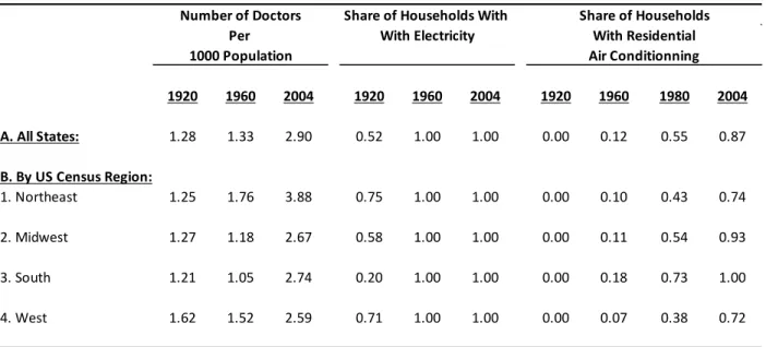
B. Summary Statistics
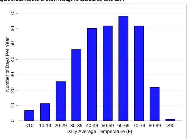
Weather and Mortality Rate Statistics. The bars in Figure 1 depict the average annual distribution of daily mean temperatures across ten temperature-day categories over the 1900-2004 period. The daily mean is calculated as the average of the daily minimum and maximum. The temperature categories represent daily mean temperatures less than 10°F, greater than 90°F, and the eight 10°F wide bins in between. The height of each bar corresponds to the mean number of days of exposure per year for the average person. In terms of “hot” temperatures, the average person is exposed to about 20 days per year with mean temperatures between 80°F and 89°F and 1 day per year where the average temperature exceeds 90°F.13
These ten bins form the basis for a simple semi-parametric modeling of temperature in equations for mortality rates that we use throughout this paper. The only substantive restriction is that the temperature-day bins restrict the marginal effect of temperature on mortality to be constant within 10°F ranges. Further, the station level temperature data is binned and then the binned data is averaged as described above; this approach preserves the daily variation in temperatures, which is important
Statistics in the United States (1958-1959). Bailey and Collins (2011) use these same data to investigate the role that electrification played in the post-World War II baby boom. The Census of Electrical Industries provides another possible electricity data source. We chose not to use these data for several reasons: They are only available every five years; much of the state data do not distinguish domestic or residential from commercial and industrial customers; and some state-year cells are suppressed or combined for confidentiality reasons.
11 The 1940, 1950, and 1960 data come from Haines (2010). For 1930 only, we digitize housing data from a printed
volume of the 1930 census. The 1930 census did not record the number of occupied dwellings. However, the 1930 census does record the number of “homes,” as distinct from the number of “dwellings.” In the Historical Statistics
of the United States (US Census 1975), the 1930 census count of “homes” is equated with the number of “occupied
housing units.”
12 As shown in Appendix Figure 3, our out-of-sample interpolations are highly correlated with independent
estimates from other national surveys.
13 Days where the daily average temperature exceeds 90°F are indeed hot. The average minimum and maximum
11
given the considerable nonlinearities in the temperature-mortality relationship (Barreca 2012, Deschenes and Greenstone 2011).
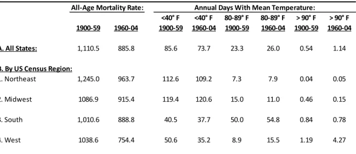
Table 1 summarizes the mortality rates and temperature variables for the whole U.S. and by Census region. To highlight differences over time, we report averages separately for the 1900-1959 and 1960-2004 periods. Over the 1900-1959 period the average annual mortality rate was 1,111 per 100,000 population, and this rate declined to an average of 885.8 over 1960-2004.
Temperatures were increasing over our sample period. Nationally, the average number of exposure days with daily average temperatures ranging from 80-89°F is 23.3 over 1900-1959 and 26.0 over 1960-2004. There is sizable geographical variation around the national average. Average exposure to 80-89 °F days in the South is about 50 days per year but only 7 in the Northeast.
There was also an increase in >90°F days over the two sample periods. There were 0.5 days and 1.1 day per year in the 1900-1959 and the 1960-2004 periods. The national mean masks important geographical variation. For example, there was almost no exposure in Northeast and little exposure in the Midwest to >90°F days. The South and West have the highest number of >90 °F days. About two-thirds of the increase in the >90°F days category in the West between the two periods reflects the relative increase in population in the hotter regions of the West.14
Modifiers of the Temperature-Mortality Relationship. Table 2 summarizes the trends in the three modifiers of the temperature-mortality relationship. It is evident that there is both geographic and time variation in the rate of diffusion of the modifiers or technologies. The subsequent analysis exploits this variation, while also adjusting for likely confounders.
Although the primary specifications in the below analysis are weighted to reflect contemporaneous population, the qualitative findings for the 1960-2004 period are unchanged by when each state’s observation is weighted by its average population from the 1900-1959 period.
Doctors Per Capita. Through the 1930s, the number of physicians per capita actually declined as the medical profession focused on training fewer individuals to a higher standard. This change was recommended in the influential 1910 Flexner Report
.
As Table 2 illustrates, the number of physicians per capita was relatively constant through 1960, at which point it began to rise (Blumenthal 2004). The current average is 2.9 doctors per 1,000 population.14 The average annual number of days experienced by the average person in the West during the 1960-2004 period
is 2.28 when the average population during the 1900-59 period is used as the weight, rather than the contemporaneous population.
12
Electrification. Table 2 reports estimates of the share of U.S. households with access to electricity from the early 1900s to 2000. Only 20% of households in the South had electricity by 1920, while more than 70% of households in the West and Northeast had access to electricity in 1920. By the early 1960s, essentially all households in the U.S. had access to electricity. Thus, estimates of the impact of electrification in modifying how temperatures affect health will be identified from variation in adoption rates in the pre-1960 period.
Residential Air Conditioning. Table 2 illustrates the fraction of households with residential AC in the United States. Prior to the mid-1950s, the share of households with AC was negligible, even though residential AC had been developed and marketed since the late 1920s. At the same time, many office buildings, movie theaters and shops offered AC to their patrons, so a large share of the population was likely aware of the benefits of this technology. In 1960, about 10% of U.S. households had a room or central AC. Following a 1957 regulatory change that allowed central AC systems to be included in FHA-approved mortgages, central air conditioning became more common (Ackermann 2002). By 1980, 50% of households lived in homes with AC and by 2004 this had increased to 87%.
Table 2 also highlights some of the key geographical differences in residential AC adoption. Although Western and Southern states were slower to receive electricity, they were quicker to adopt AC. Residential AC is more likely to offer indoor comfort and possibly health benefits to a resident of a warm climate than to a resident of a more moderate climate.
IV. Econometric Approach
The regression models are identified by plausibly random inter-annual variation in state by month temperature distributions. Specifically, we estimate versions of the following equation:
where log(Ysym) is the log of the monthly mortality rate in state s, year y, and month m. The vector of control variables, Xsy, includes log per-capita income, the share of the population living in urban areas, and the share of the state population in one of four age categories: infants (0-1); 1-44; 45-64; and 65+
13
years old.15 The vector also includes interactions of log per capita income with calendar month to
account for the possibility that changes in annual income provide relatively greater health benefits across months of the year.16
The specification also includes a full set of state-by-month fixed effects (αsm) and year-month
fixed effects (γym). The state-by-month fixed effects are included to absorb differences in seasonal
mortality (which is the largest in the winter months and smallest in the summer months) across states in a way that is correlated to climatic seasonality. They control for all unobserved state-by-month time invariant determinants of the mortality rate, so, for example, fixed differences in hospital quality or the level of health capital will not confound the weather variables. The year-by-month fixed effects control for idiosyncratic changes in mortality outcomes that are common across states (e.g., the introduction of Medicare and Medicaid).
Further, the preferred specification includes a quadratic time trend that is allowed to vary at the state-month level to control for smooth changes in the state-by-month mortality rate across years. These trends will control for local factors that affect mortality (possibly in a seasonal manner), such as air pollution.
The variables LOWPsym and HIGHPsym are indicators for unusually high or low amounts of
precipitation in the current state-year-month. More specifically, these are defined as indicators for realized monthly precipitation that is less than the 25th (LOWP
sym) or more than the 75th (HIGHPsym)
percentiles of the 1900-2004 average monthly precipitation in a given state-month. In the interest of space, we do not report the estimated coefficients.
The variables of central interest are the measures of temperature TMEANsymj. These TMEAN variables are constructed to capture exposure to the full distribution of temperature and are defined as the number of days in a state-year-month where the daily mean temperature is in the jth of the 10 bins used in Figure 1. In practice, the 60°F – 69°F bin is the excluded group, so the coefficients on the other bins are interpreted as the effect of exchanging a day in the 60°F – 69°F bin for a day in other bins. The primary functional form restriction implied by this model of temperature exposure is that the impact of the daily mean temperature on the monthly mortality rate is constant within 10°F degree intervals. The choice of 10 temperature bins represents an effort to allow the data, rather than parametric assumptions, to determine the mortality-temperature relationship, while also obtaining estimates that are precise enough that they have empirical content.
15 There is no data available at state-year-month level that identifies vital events separately for rural and urban
populations. As such, we control for urban population shares in all specifications to account for the possibility that urbanization is spuriously correlated with temperature changes.
14
We also use a more parsimonious model that focuses entirely on the upper and lower tails of the daily temperature distribution. Specifically, we focus on four temperature-bin variables: the number of days below 40°F; the number of days between 80°F and 89°F; and the number of days above 90°F. Thus, the number of days in the 40°F – 79°F bin is the excluded category here. This choice of degree-days bins is informed by the estimated response function linking mortality and the 10 temperature-day bins. As we show below, estimates of the θ parameters associated with high daily temperatures (i.e., 80°F – 89°F and >90°F) are very similar to the 4 and 10 bin approaches, so the more parsimonious approach does not materially affect the conclusions.
Importantly, the preferred empirical estimates account for inter-temporal mortality displacement, or “harvesting”, of persons who are ill and already near death. One potential concern is that periods of unusually high temperature lead to short-term spikes in daily or weekly mortality that are followed by several days of below trend mortality. Therefore, examining the day-to-day correlation between mortality and temperature will overstate the substantive effect of temperature on life expectancy. In addition, the possibility of delayed effects can also confound the day-to-day temperature mortality association. To address this empirical issue, the preferred specification includes an exposure window of 2 months, which includes the month a mortality event is registered and the previous month. This is a longer exposure window than in most of the previous literature, but, as we find below, the choice of 1 or 2 months for the exposure window does not qualitatively change the main results.17
Two additional econometric issues bear noting. First, the standard errors are clustered at the state level, which allows the errors within states to be arbitrarily correlated over time. Second, we estimate the models using GLS, where the weights correspond to the square root of the contemporaneous state population. The estimates of mortality rates from large population states are more precise, so GLS corrects for heteroskedasticity associated with these differences in population size. Further, the GLS results reveal the impact on the average person, rather than on the average state.
Longer exposure windows are examined as a robustness check.
Finally, to quantify the contribution of each specific innovation to the change in the temperature-mortality relationship, Equation (1) is augmented by interacting the temperature variables with state-by-year measures of log doctors per capita, the fraction of households with electricity, and the fraction of households with residential AC. The main effects for these variables are also included in
17 Most papers in the epidemiology literature consider displacement windows of less than 3 weeks. Deschenes and
Moretti (2009) use a window of one month in their baseline specification, Barreca (2012) uses a two-month exposure window, and Deschenes and Greenstone (2011) implicitly use a window of up to one year.
15
the specification. We posit that the coefficients on the interaction terms will be negative at the extreme temperature categories. A negative coefficient would be interpreted as evidence that the diffusion of a particular modifier reduced a population’s relative vulnerability to temperature extremes. In particular, the modifier variables are expected to play a key role in dampening the mortality effects of high temperatures (e.g. days >90°F). Further, some of the interactions should not affect mortality due to low temperatures and the coefficients on these interactions (e.g., AC * days <40°F) serve as robustness checks.
V. Results A. Estimates of the Temperature-Mortality Relationship
Daily Mean Temperatures. Figure 2 (a) presents estimates of the temperature-mortality relationship from the fitting of the 10 bin version of Equation (1) to data from 1900-2004. The temperature exposure window is 1 month. The specification includes all the control variables described in the econometrics section (except per capita income because it is only available from 1929 onwards): state-by-month fixed effects; year-by-month fixed effects; and a quadratic time trend that is allowed to vary at the state-by-month level. The figure plots the regression coefficients associated with the temperature-day bins (i.e., the θj’s) where the 60°F – 69°F temperature bin is the reference (omitted) category.18
The figure confirms that mortality risk is highest at the temperature extremes, and particularly so for temperatures above 90°F. The point estimates underlying the response function indicate that exposure to one day above 90°F increases the mortality rate by approximately 1.1% (i.e., 0.011 log mortality points), while exposure to the 80°F – 89°F category increases the mortality rate by about 0.3%. Cold temperatures also lead to excess mortality: The coefficients associated with the lowest three temperature bins range from 0.5% to 0.7%. All estimates associated with temperature exposures above 80°F and below 50°F are statistically significant at the 5% level. This U-shaped relationship is consistent with previous temperature-mortality research (see Deschenes 2012 and NIEHS 2010 for reviews of the literature), although these are the first comprehensive estimates of the temperature-mortality That is, each coefficient measures the estimated impact of one additional day in temperature bin j on the log monthly mortality rate, relative to the impact of one day in the 60°F – 69°F range.
18A normalization is needed since the number of days in a given month is constant and the temperature-day bins
16
relationship over the entire 20th century. The estimates in Figure 2 (a) also motivate the more parsimonious approach to modeling temperature with 4 bins instead of 10.
Figure 2 (b) plots estimates based on the same specification as 2 (a), except that controls for interactions between log per capita income and month are added to the model. Since the data on per capita income are only available from 1929 onwards, the sample period is 1929-2004. Comparison between Figures 2 (a) and (b) make it evident that the estimates are robust to controlling for log per capita income.
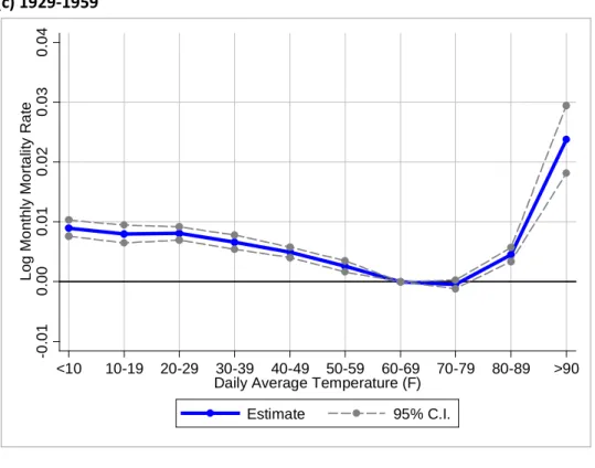
Figures 2 (c) and (d) illustrate how temperature-mortality has changed over time. Specifically, they plot the estimated coefficients on the temperature variables from the fitting of a version of Equation (1) on data for the 1920-1959 and 1960-2004 periods. The estimates are adjusted for the same controls as in Figure 2 (b). The “breakpoint” of 1960 was chosen because 100% of households had electricity but a small fraction had residential AC as of 1960.
Two key results emerge from Figures 2 (c) and (d). First, there is a sharp decline in the mortality impact of high temperature days (especially those above 90°F) after 1960. Second, there is a smaller decline at low temperatures.
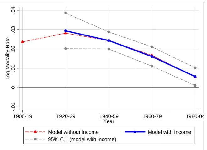
Figure 3 explores the decline in the mortality impact of temperature days above 90°F in greater detail. Specifically, it estimates the temperature-mortality relationship based on the 10 bins and preferred specification of Equation (1) for 20-year periods: 1900-1919, 1920-1939, 1940-1959, 1960-1979, and 1980-04. Two sets of estimates are reported. Estimates denoted by the red line (triangle markers) are based on models that exclude month*log per capita income interactions (but include all other controls, fixed effects and interactions described along Equation [1]). Estimates denoted by the blue line (blue markers) are based on models that add month*log per capita income interactions to the specification. The latter specification can only be estimated from 1929 onwards, so effectively the first period for is 1929-1939.
The key results are as follows: First, the inclusion or exclusion of month*log per capita income interactions is inconsequential for the evolution of the relationship between high temperatures (days exceeding 90°F) and mortality. Second, the estimated effect of temperature-days exceeding 90°F remains roughly constant at around 0.025-0.03 log mortality points (so about a 2.5-3% effect on the mortality rate) from 1900 to 1959, and then begins a sharp decline over the period 1960-2004. As we substantiate below, this decline coincides with the diffusion of residential AC in the United States.
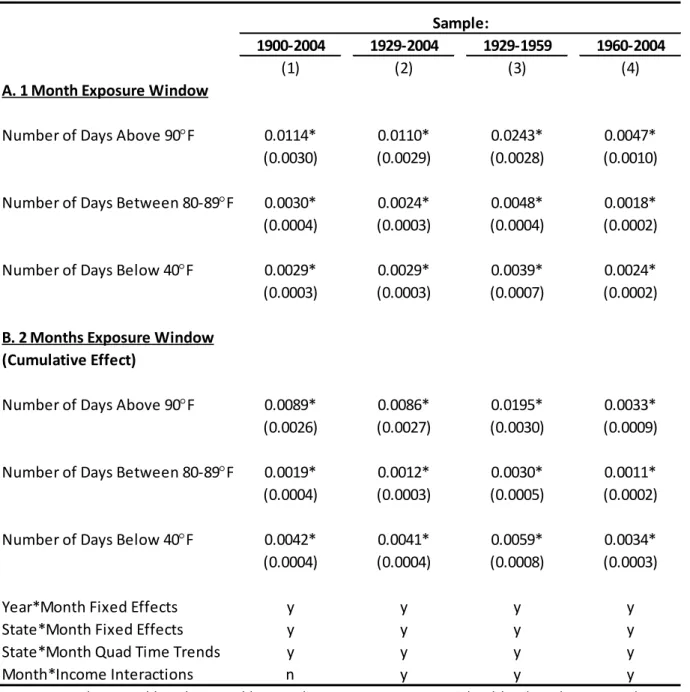
Table 3 provides an opportunity to precisely summarize the qualitative impressions from Figures 2 and 3. It reports estimates from the version of Equation (1) that models temperature with four
17
temperature-bin variables: the number of days below 40°F; the number of days between 80°F – 89°F; and the number of days above 90°F (the number of days with mean temperature between 40°F – 79°F is excluded). This simpler functional form is motivated by the estimates in Figure 2 that suggested that the θj’s were approximately equal in the below 40°F and 40°F - 79°F categories. In Panel [A], the exposure window is the current month’s temperature only as in Figures 2 and 3. Panel [B] reports cumulative dynamic estimates based on models that control for two months of temperature exposure. The cumulative dynamic estimates allow the effect of the temperature bins to differ in the current and previous months and then we sum each the coefficients of each temperature-day bin variable from the current and previous months. In the robustness analysis below we extend the displacement window to four months.
All estimates in Table 3 are derived from the preferred specification of Equation (1) that includes the full set of covariates, state*month fixed effects, year*month fixed effects, and a quadratic time trend that is allowed to vary at the state*month level. The four columns of Table 3 correspond to the different estimation periods: 1900-2004, 1929-2004, 1900-1959, and 1960-2004. The specifications underlying the estimates in columns (2) - (4) include controls for log per capita income interacted with month.
The results in Panel A of Table 3 confirm the above findings that temperature extremes increase mortality risk and that there was a dampening in the temperature mortality relationship over time. For example, over the course of the 20th century, the exchange of a day in the range of 40°F - 79°F for one with a mean temperature above 90°F leads to a 1.1 percent increase in annual mortality. A comparison of columns (3) and (4) reveals that this effect declined by more than 80% between the 1929-1959 and 1960-2004 periods (from 2.43% to 0.47%). Exposure to temperature-days between 80-89°F and temperature-days below 40°F also leads to statistically significant increases in mortality, but the effects are much smaller. Further, the impacts of temperatures in these ranges declined after 1959, but the declines were more modest than the decline for >90°F days; this is true both in levels and percentage declines, which were 60% for 80°F – 89°F days and 40% for temperature-days below 40°F).
Panel B uses a two-month exposure window and is, therefore, more robust to near-term mortality displacement. The estimates in Panel B are generally slightly smaller in absolute terms than those in Panel A, indicative of some degree of near-term displacement or measurement error. However, it is clear that the 95% confidence intervals for the Panel A and B estimates all overlap. Nonetheless, the magnitudes of the >90°F temperature-day exposure on mortality remain large and all are statistically significant at the 5% level. In addition, the decline in the mortality effect of these days is also greater
18 than 80% after 1959.19
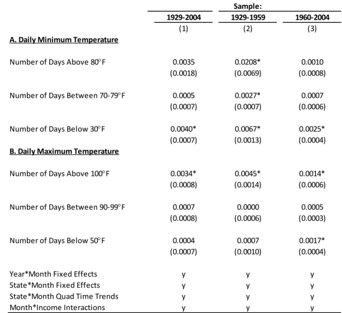
Minimum and Maximum Temperatures. Table 4 reports on a specification that includes daily minimum and maximum temperatures but is otherwise identical to the one used in columns (2) - (4) of Table 3. This specification allows for an examination of potential non-linear effects at temperature extremes missed in the mean temperature analyses.
We proceed with the two-month exposure window for the remainder of this paper since the model better addresses near-term displacement.
20
In interpreting the results in Table 4, it is important to note that minimum temperatures are typically achieved at nighttime, as opposed to daytime for maximum temperatures. One potential explanation of these results is that the reduction in the mortality impact of high temperatures is due to changes in health-producing behaviors at home, instead of the workplace. It therefore seems plausible that increased usage of residential AC led to reduced thermal stress at night. However, varying daily minimum temperature while holding daily maximum temperature constant also leads to changes in the spread of temperatures, humidity, and rainfall, which might affect mortality independent of the daily minimum. We investigate the role of residential AC in the below.
There is a large decline in the effects of daily minimum temperatures above 80°F in the later period; for example, the coefficient declines from 0.0208 to 0.0010, or a decline of roughly 90%. The impact of days above 100°F declined from 0.45% to 0.14%, or a nearly 70% decline. Thus, using diurnal temperatures, we confirm our core findings above that there was a dampening of the temperature-mortality relationship at high temperatures.
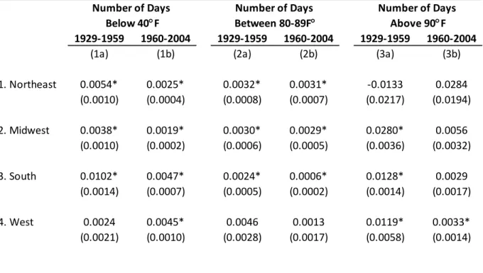
Heterogeneity by Region. Table 5 estimates the temperature-mortality relationship by census region. One hypothesis is that areas that are more accustomed to temperature extremes may have adapted better, and thus, have a muted temperature-mortality relationship. For example, the populations of these regions may have adopted different technologies (e.g. better insulation) or are more familiar with the need for proper hydration.
There is substantial heterogeneity in the estimated effects of extreme temperatures on mortality across regions. For example, the impact of temperature-days exceeding 90°F is largest in the Midwest region, where exposure is relatively infrequent. Similarly, exposure to cold temperature days leads to larger mortality impacts in the South region, where again exposure is infrequent. The estimates for temperature-days >90°F in the Northeast are statistically imprecise since such days were extremely
19 Malaria cannot explain the dampening of the temperature mortality relationship. Malaria was mostly confined
to the South by 1920 (Maxcy 1923). Also, the South had nearly eradicated malaria by 1940 (Barreca et al. 2012). The fact that we observe a dampening of the temperature-mortality relationship both: a) outside the South, and b) after 1940, suggests that malaria’s eradication cannot account for the majority of our estimates.
20 Results are similar when we control for daily minimum and maximum temperature-bins in the same regression
19
rare (the average number of such days in the Northeast region is about 0.05 – or 1 day per 20 years. The decline in the mortality impacts of >90°F days across the Midwest, South, and West are similar to our core estimates in Table 3. That is, the structural change in the temperature-mortality relationship appears similar across the different regions of the United States.
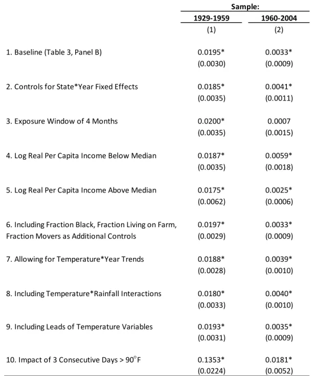
Robustness tests. Table 6 probes the robustness of the estimated effect of >90°F days on
mortality. We vary the control variables, subsamples, and fixed effects. The estimates are derived from the full 1929-1959 and 1960-2004 samples when information on per capita income is available. The columns report the estimated coefficients for the two sample periods. Estimates in Table 6 are based on the models with a two-month exposure window.
The first row reproduces the baseline estimates from Table 3.21 Row 2 replaces the
state-by-month quadratic time trends with state-by-year fixed effects. Row 3 returns to the baseline specification, but uses a four-month exposure window and reports the corresponding cumulative estimate. Rows 4 and 5 stratify the sample by median per capita income.22 Row 6 is similar to our core
model (row 1), but add controls for state-year estimates of the fraction living on farms, the fraction black, and the fraction of state residents born in a different state.23
The specification in row 7 allows the impact of >90°F temperature-days on mortality to parametrically change over time (separately for the 1929-1959 and 1960-2004 samples) by adding interactions of calendar year with each of the temperature variables. The temperature-by-year trends capture the effect of all confounders that lead to a gradual reduction of the mortality effect of high temperature-days, for example the gradual improvement in air quality in the United States from the early 1970s onwards. The marginal effect reported in the table shows that our baseline estimates are not driven by such omitted factors.
We include them as controls because changes in exposure to temperature extremes in the workplace (i.e., farming), differential access to health care by race (Almond, Chay and Greenstone 2007), and changes in migration patterns may confound the measured change in the temperature-mortality relationship. The estimates are robust to all of these alterations to the baseline model.
The row 8 specification adds interactions between the temperature variables and the precipitation variables (LOWP and HIGHP) and reports the marginal effects evaluated at the sample
21 In this baseline specification, the coefficient associated with “low” monthly precipitation (deviation from
state-month average in the lowest tercile) is statistically significant at 0.0027 (se = 0.0007). The coefficient on “high” monthly precipitation is smaller and statistically insignificant (-0.0003).
22 The medians are calculated over all sample years (and weighted by population), so the assignment of a state to a
below or above median group remains constant across all years.
20
means. This addresses the possibility of temperature effects that depend on the degree of humidity, as warmer and wetter days are generally humid. This leads is no meaningful change in the effects of >90°F days.
Row 9 is based on the same specification as row 1, except it includes leads of the temperature variables in addition to the values for the current and previous month. We include leads as a “placebo” test: Any significant difference in the estimates from the “with leads” and “without leads” models would be an indication of the main results being driven by trends or factors that we fail to control for. Our estimates pass this placebo test. Also, F-tests indicate that the leads do not enter the models significantly.24
Finally, in row 10 we consider the impact of “heat waves”, which are defined as 3 consecutive days or more where the average temperature exceeds 90°F. Specifically, we replace the temperature variables with the number of episodes of 3 days in a row of <40°F, 80°F – 89°F, and >90°F. On average, heat waves occur once every 8.3 years (the sample average is 0.12 heat waves per year). This analysis is motivated by the prior epidemiological literature which found that exposure to consecutive days of high temperature has a stronger effect on mortality than exposure to “isolated” high temperature days. Our estimates in row 9 confirm this finding and also support the key finding of a large reduction in the mortality effect of high temperature exposure after 1960. The estimated coefficient for the mortality effect of heat waves declines from 13.5% before 1960 to 1.8% after 1959, which is a reduction of 87%.
In sum, our robustness checks support the hypothesis that there was a significant dampening of the temperature-mortality relationship.25 Further, this dampening was relatively greater at high
temperatures. The next subsection explores the roles of increased access to health care, residential electricity, and residential air conditioning (AC) in muting the temperature-mortality relationship.
24The F-statistics testing that the lead coefficients on number of days below 40°F, number of days between 80°F –
89°F, and number of days above 90°F are 0.57 (column 1) and 2.09 (column 2), with p-values of 0.64 and 0.11, respectively.
25 We also performed other robustness analyses that are not reported here due to space limitations. Specifically,
we have re-estimated the baseline specification for 1960-2004 using 1940 population weights (as opposed to annual population weights for all sample years). The year 1940 was chosen as it pre-dated the central city to suburban areas mobility that began in the 1950s (see e.g., Baum-Snow 2007). Such mobility could confound our estimates if urban heat island effects are important enough, and if suburban mobility reduces high temperature exposure (see Arnfield 2003 for a review of urban heat island studies). The estimates from regressions weighted by the fixed 1940 population are the same as those reported in row 1 of Table 6, so central city to suburban mobility is unlikely to be a driver of the results presented here. Alternatively, we also introduced interactions between population density and the temperature variables in the baseline model. These interactions fail to enter statistically significantly in all estimated models.
21
B. The Impact of the Modifiers of the Temperature-Mortality Relationship
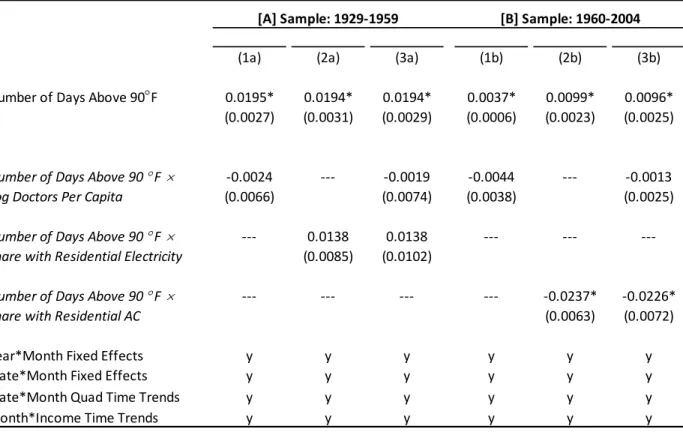
Table 7 reports on a specification that adds the main effects for the three modifiers and their interactions with the three daily temperature variables to the parsimonious temperature specification. All of the standard controls used in Table 3 Panel B are included. For brevity, the table only reports the effect of temperature-days >90°F and the coefficients on the interactions of this variable with the modifiers. These coefficients are most relevant for the impacts of climate change, but the corresponding coefficients for the other temperature variables are reported in Appendix Tables 5 and 6.
Panel A focuses on the period 1929-1959, and Panel B analyzes the 1960-2004 data. The cutoff date is 1960, since in 1960 virtually all households in the United States had access to electricity and few households had air conditioning. For this reason, the estimated modifying effect of electrification is only reported in Panel A (sample years 1929-1959), and the estimated modifying effect of residential AC is only reported in Panel B (sample years 1960-2004). The protective effect of doctors per capita is measured in both samples. We consider specifications with the effect of each modifier individually as well as jointly.
Over the period 1929-1959, the modifiers appear to have little measurable effect on mortality. The effect of doctors in columns (1a) and (3a) is negative, but not significant and small. The estimated effect of electricity in columns (2a) and (3a) is positive, which is perversely signed as it indicates that electricity increased the mortality impact of high temperature days. These estimates are of a substantial magnitude but would not be judged to be statistically significant by conventional criteria. Appendix Table 6 shows that electrification leads to a statistically significant decline in cold-related mortality (i.e., mortality due to temperature-days less than 40°F).
Over the period 1960-2004, air conditioning appears to have had a sizeable and statistically significant negative effect on mortality. The effect of doctors remains negative, but not significant and small. The estimates in columns (2b) and (3b) suggest that each 10 percentage point increase in residential AC ownership decreased the high temperature mortality effect by 0.002, or roughly 10 percent of the effect of a >90°F temperature day in the pre-1960 period. Put another way, the regressions imply that if residential AC increased from covering none of the population to covering 59% of the population (the average share of the population with residential AC in our sample) but everything else remained fixed, the effect of temperature-days >90°F on log mortality rates would have fallen by 0.0140 (= 0.59*0.0237). By contrast, in Table 3, the actual decline in the effect of temperature-days >90°F on log mortality rates between the periods 1900-1959 and 1960-2004 is 0.0162 (= 0.0195-0.0033).
22
Hence, residential AC alone can explain about 86 percent of the decline in extreme heat’s effect on mortality during the 20th century. 26
Tables 8 and 9 present the modifier analysis by age group, by race, and by cause of death. Table 8 provides support for the hypothesis that there is a strong protective effect of the modifiers in vulnerable populations. The estimates in column (3), which are adjusted for doctors per capita, show that the effects of air conditioning in mitigating the mortality impact of days with temperatures exceeding 90°F are large and statistically significant for infants and the elderly. The infant estimates are consistent with the hypothesis that infants’ thermoregulatory systems are not yet fully functional (Knobel and Holditch-Davis 2007). The Table 9 entries suggest that the protective effect of residential AC against days with temperatures exceeding 90°F is larger for blacks than whites, although the 95% confidence intervals overlap.
Table 10 provides support that the protective effects of AC are operating through reduced exposure to heat stress. We find that AC reduces the impacts of >90°F days on cardiovascular-related and respiratory-related mortality. In contrast, there is no significant effect on fatalities due to motor vehicle accidents or infectious disease, suggesting that the AC results do not simply reflect a trend in mortality. We do find that AC reduces the impacts of >90°F days on neoplasm mortality. In supplementary analysis (not reported), we found this result to be driven entirely by the 65-74 age group, and so the result is only salient to a very specific population.
VI. Interpretation
The paper’s results can be interpreted in several lights. Perhaps the most straightforward is to turn these changes in mortality rates into more concrete or meaningful measures. During the 1929-1959 period, the United States population was on average 142.5 million and the typical American experienced 1.03 day per year where the temperature exceeded 90°F. Taking the estimates in Table 3 Panel B literally, there were approximately 1,600 premature fatalities annually due to high temperatures in this period. The available data do not allow for a precise calculation of the loss in life expectancy, but due to the choice of the specification these were not gains of a few days or weeks: all were of a
26 We also experimented with a specification that adds a year trend interaction to each of the temperature
variables’ main effects, in addition to the modifier interactions. The resulting estimate of the heat-protective effect of residential AC remains significant and is similar in magnitude of the ones reported in Table 7. Thus the estimates of the protective effect of residential AC in Table 7 are unlikely to be driven by unobserved factors that lead to a gradual reduction of the mortality effect of high temperature-days.
23
minimum of two months. It seems reasonable to presume that the loss of life expectancy for infants (recall Table 8) was substantially longer than two months, perhaps even full lives. Obviously, the number of saved lives would be larger if the impact of days in the 80°F – 89°F range were included in this calculation.
By comparison, during the 1960-2004 period, there were on average 232.2 million Americans and they faced an average of 1.14 days with temperatures above 90°F. The analogous calculation using the estimates in Table 3 Panel suggests that there were roughly 600 premature fatalities annually due to high temperatures in this period. If the earlier period’s mortality impact of hot days prevailed over 1960-2004, the annual number of premature fatalities would have been about 3,600.
What role did air conditioning play in this dramatic reduction in vulnerability to hot temperature days? Using our estimates of the protective effect of residential AC on days exceeding 90°F from Table 7 we find that the diffusion of residential AC during the 1960-2004 led to an avoidance of 3,300 annual premature fatalities. It is apparent that residential air conditioning has a tremendous positive impact on well being.
A second way to illustrate these results is to underscore how air conditioning has positioned the United States to be well adapted to the temperature-related mortality impacts of climate change.27
While residential AC appears to provide U.S. residents with great protection against temperature-related mortality, many other countries are currently vulnerable; this is especially the case for poor countries in the tropics. As just one measure of the stakes, the typical Indian experiences 33 days annually where the temperature exceeds 90°F and this is projected to increase by as much as 100 days by the end of the century (Burgess et al. 2011). Indeed, using data from 1957-2000, Burgess et al. (2011) find that one additional day above 90°F, compared to a day in the 60°F – 69°F range, increases State of the art climate change models with business as usual scenarios predict that the United States will have 42.3 additional days per year where the temperature exceeds 90°F by end of the century (see e.g., Deschenes and Greenstone 2011). If residential AC adoption were at the 1960 rate of adoption and population was at 2004 levels, then the 1960-2004 Table 7 estimates suggest that the increase in >90°F days would cause an additional 59,000 deaths annually by the end of the century. However, at 2004 rates of residential AC adoption, the null hypothesis that additional extremely hot days would have no impact on mortality cannot be rejected with the available estimates.
27 Of course, residential air conditioning will not be protective for many other manifestations of climate change,