Semi-empirical modeling of abiotic and biotic factors controlling ecosystem respiration across eddy covariance sites

HAL Id: hal-00599515

https://hal.archives-ouvertes.fr/hal-00599515

Submitted on 10 Jun 2011

HAL is a multi-disciplinary open access archive for the deposit and dissemination of sci-entific research documents, whether they are pub-lished or not. The documents may come from teaching and research institutions in France or abroad, or from public or private research centers.

L’archive ouverte pluridisciplinaire HAL, est destinée au dépôt et à la diffusion de documents scientifiques de niveau recherche, publiés ou non, émanant des établissements d’enseignement et de recherche français ou étrangers, des laboratoires publics ou privés.

sites

Mirco Migliavacca, Markus Reichstein, Andrew D. Richardson, Roberto

Colombo, Mark A. Sutton, Gitta Lasslop, Georg Wohlfahrt, Enrico Tomelleri,

Nuno Carvalhais, Alessandro Cescatti, et al.

To cite this version:

Mirco Migliavacca, Markus Reichstein, Andrew D. Richardson, Roberto Colombo, Mark A. Sut-ton, et al.. Semi-empirical modeling of abiotic and biotic factors controlling ecosystem respiration across eddy covariance sites. Global Change Biology, Wiley, 2010, 17 (1), pp.390. �10.1111/j.1365-2486.2010.02243.x�. �hal-00599515�

For Review Only

Semi-empirical modeling of abiotic and biotic factors controlling ecosystem respiration across eddy covariance

sites

Journal: Global Change Biology Manuscript ID: GCB-10-0015

Wiley - Manuscript type: Primary Research Articles Date Submitted by the

Author: 07-Jan-2010

Complete List of Authors: Migliavacca, Mirco; University of Milano-Bicocca, Remote Sensing of Environmental Dynamics; Max Planck Institute for Biogeochemistry, Model Data Integration Group

Reichstein, Markus; Max Planck Institute for Biogeochemistry, Model Data Integration Group

Richardson, Andrew; Harvard University, Department of Organismic and Evolutionary Biology

Colombo, Roberto; University of Milano-Bicocca, Remote Sensing of Environmental Dynamics

Sutton, Mark A.; Centre for Ecology and Hydrology, Edinburgh Research Station

Lasslop, Gitta; Max Planck Institute for Biogeochemistry, Model Data Integration Group

Wohlfahrt, Georg; University of Innsbruck, Institute of Ecology Tomelleri, Enrico; Max Planck Institute for Biogeochemistry, Model Data Integration Group

Carvalhais, Nuno; Universidade Nova de Lisboa, Faculdade de Ciências e Tecnologia; Max Planck Institute for Biogeochemistry, Model Data Integration Group

Cescatti, Alessandro; European Commission, DG-JRC, Institute for Environment and Sustainability

Mahecha, Miguel; Max Planck Institute for Biogeochemistry, Model Data Integration Group; Swiss Federal Institute of Technology-, Department of Environmental Sciences

Montagnani, Leonardo; Provincia Autonoma di Bolzano, Agenzia per l'Ambiente, Servizi Forestali

Papale, Dario; University of Tuscia, DISAFRI

Zaehle, Sönke; Max Planck Institute for Biogeochemistry, Department for Biogeochemical System

Arain, M Altaf; McMaster University, School of Geography & Earth Sciences

Arneth, Almut; Lund University, 13- Department of Physical Geography and Ecosystems Analysis

For Review Only

Black, T Andrew; University of British Columbia, Faculty of Land and Food Systems

Dore, Sabina; Northern Arizona University, School of Forestry Gianelle, Damiano; Fondazione Edmund Mach, Centro di Ecologia Alpina

Helfter, Carole; Centre for Ecology and Hydrology, Edinburgh Research Station

Hollinger, David; USDA Forest Service, NE Research Station Kutsch, Werner; Johann Heinrich von Thünen Institut, Institut für Agrarrelevante Klimaforschung

Law, Beverly; Oregon State University, College of Forestry Lafleur, Peter M; Trent University, 20- Department of Geography Nouvellon, Yann; CIRAD, Persyst

Rebmann, Corinna; Max-Planck Institute for Biogeochemistry, Biogeochemical Processes; University of Bayreuth, Department of Micrometeorology

da Rocha, Humberto; Universidade de São Paulo, Dept. of Atmospheric Sciences

Rodeghiero, Mirco; Fondazione Edmund Mach, Centro di Ecologia Alpina

Olivier, Roupsard; CIRAD, Persyst; Centro Agronómico Tropical de Investigación y Enseñanza, CATIE

Sebastià, Maria-Teresa; University of Lleida, Agronomical Engineering School; Forest Technology Centre of Catalonia, Laboratory of Plant Ecology and Botany

Seufert, Guenther; Institute for Environment and Sustainability, European Commission, DG-JRC

Soussana, Jean-Francoise; Institut National de la Recherche Agronomique

van der Molen, Michiel K; University de Boeleaan, Department of Hydrology and Geo-Environmental Sciences

Keywords: Ecosystem Respiration, Productivity, FLUXNET, Eddy Covariance, Leaf Area Index, Inverse Modeling

Abstract:

In this study we examined ecosystem respiration (RECO) data from 104 sites belonging to FLUXNET, the global network of eddy covariance flux measurements. The main goal was to identify the main factors involved in the variability of RECO: temporally and between sites as affected by climate, vegetation structure and plant functional type (PFT) (evergreen needleleaf, grasslands, etc.). We demonstrated that a model using only climate drivers as predictors of RECO failed to describe part of the temporal variability in the data and that the dependency on gross primary production (GPP) needed to be included as an additional driver of RECO. The maximum seasonal leaf area index (LAIMAX) had an additional effect that explained the spatial variability of reference respiration (the respiration at reference temperature Tref=15°C, without stimulation introduced by photosynthetic activity and without water limitations), with a statistically significant linear relationship

(r2=0.52 p<0.001, n=104) even within each PFT. Besides LAIMAX, we found that the reference respiration may be explained partially by total soil carbon content. For undisturbed temperate and boreal forest a negative control of the total nitrogen deposition on the reference respiration was also identified.

We developed a new semi-empirical model incorporating abiotic factors (climate), recent productivity (daily GPP), general site productivity and canopy structure (LAIMAX) which performed well in predicting the spatio-temporal variability of RECO, explaining >70% of the variance for most vegetation types. Exceptions include tropical and Mediterranean broadleaf forests and deciduous

3 4 5 6 7 8 9 10 11 12 13 14 15 16 17 18 19 20 21 22 23 24 25 26 27 28 29 30 31 32 33 34 35 36 37 38 39 40 41 42 43 44 45 46 47 48 49 50 51 52 53 54 55 56 57 58 59 60

For Review Only

broadleaf forests. Part of the variability in respiration that could not be described by our model could be attributed to a range of factors, including phenology in deciduous broadleaf forests and

management practices in grasslands and croplands. 3 4 5 6 7 8 9 10 11 12 13 14 15 16 17 18 19 20 21 22 23 24 25 26 27 28 29 30 31 32 33 34 35 36 37 38 39 40 41 42 43 44 45 46 47 48 49 50 51 52 53 54 55 56 57 58 59 60

For Review Only

1

Semi-empirical modeling of abiotic and biotic factors controlling ecosystem

respiration across eddy covariance sites

3

Mirco Migliavacca1,2, Markus Reichstein2, Andrew D. Richardson3, Roberto Colombo1, Mark A. 4

Sutton4, Gitta Lasslop2, Georg Wohlfahrt5, Enrico Tomelleri2, Nuno Carvalhais6,2, Alessandro 5

Cescatti7, Miguel D. Mahecha2,8, Leonardo Montagnani9, Dario Papale10 , Sönke Zaehle 11, Altaf 6

Arain12, Almut Arneth13, T. Andrew Black14, Sabina Dore15, Damiano Gianelle16, Carole Helfter4, 7

David Hollinger17, Werner L. Kutsch18, Beverly E. Law19, Peter M. Lafleur20, Yann Nouvellon21, 8

Corinna Rebmann22,23, Humberto Ribeiro da Rocha24, Mirco Rodeghiero16, Olivier Roupsard21,25, 9

Maria-Teresa Sebastià26,27_{, Guenther Seufert}7_{, Jean-Francoise Soussana}28_{, Michiel K. van der} 10

Molen29 11

12

1- Remote Sensing of Environmental Dynamics Laboratory, DISAT, University of Milano-13

Bicocca, Milano, Italy. 14

2- Model Data Integration Group, Max Planck Institute for Biogeochemistry, Jena, Germany. 15

3- Department of Organismic and Evolutionary Biology, Harvard University, Cambridge MA, 16

USA. 17

4- Centre for Ecology and Hydrology, Edinburgh Research Station, Bush Estate, Penicuik, 18

Midlothian, Scotland, EH26 0QB, UK. 19

5- Institut für Ökologie, Universität Innsbruck, Innsbruck, Austria. 20

6- Faculdade de Ciências e Tecnologia, FCT, Universidade Nova de Lisboa, 2829-516, 21

Caparica, Portugal. 22

7- European Commission, DG-JRC, Institute for Environment and Sustainability, Climate 23

Change Unit, Via Enrico Fermi 2749, T.P. 050, 21027 Ispra (VA), Italy. 24

8- Department of Environmental Sciences, Swiss Federal Institute of Technology-ETH Zurich, 25

8092 Zurich, Switzerland. 26

9- Agenzia Provinciale per l'Ambiente, Via Amba-Alagi 5, 39100 Bolzano, Italy. 27

10- DISAFRI, University of Tuscia, via C. de Lellis, 01100 Viterbo Italy. 28

11- Department for Biogeochemical System, Max Planck Institute for Biogeochemistry, Jena, 29

Germany. 30

12- McMaster University, School of Geography & Earth Sciences, 1280 Main Street West, 31

Hamilton, ON, L8S 4K1, Canada. 32

13- Department of Physical Geography and Ecosystems Analysis, Lund University, Sölvegatan 33

12, SE-223 62 Lund, Sweden. 34

14- Faculty of Land and Food Systems, University of British Columbia, Vancouver, BC, 35

Canada. 36

15- Department of Biological Sciences and Merriam-Powell Center for Environmental 37

Research, Northern Arizona University, Flagstaff, Arizona, USA. 38

16- IASMA Research and Innovation Centre, Fondazione E. Mach, Environment and Natural 39

Resources Area, San Michele all’Adige, I-38040 Trento, Italy 40

17- USDA Forest Service, NE Research Station, Durham, NH, USA 41

18- Johann Heinrich von Thünen Institut (vTI), Institut für Agrarrelevante Klimaforschung, 42

Braunschweig, Germany 43

19- College of Forestry, Oregon State University, 97331-5752 Corvallis, OR, USA 44

20- Department of Geography, Trent University, Peterborough, ON K 9J 7B8, Canada. 45

21- CIRAD, Persyst, UPR80, TA10/D, 34398 Montpellier Cedex 5, France. 46

22- University of Bayreuth, Department of Micrometeorology, Bayreuth, Germany. 47

23- Max Planck Institute for Biogeochemistry, Jena, Germany. 48

24- Departamento de Ciências Atmosféricas/IAG/Universidade de São Paulo, Rua do Matão, 49

1226 - Cidade Universitária - São Paulo, SP - Brasil. 50 3 4 5 6 7 8 9 10 11 12 13 14 15 16 17 18 19 20 21 22 23 24 25 26 27 28 29 30 31 32 33 34 35 36 37 38 39 40 41 42 43 44 45 46 47 48 49 50 51 52 53 54 55 56 57 58 59 60

For Review Only

2

25- CATIE, Centro Agronómico Tropical de Investigación y Enseñanza, Turrialba Costa Rica. 51

26- Laboratory of Plant Ecology and Botany. Forest Technology Centre of Catalonia, Solsona, 52

Spain. 53

27- Agronomical Engineering School, University of Lleida, E-25198 Lleida, Spain. 54

28- INRA, Institut National de la Recherche Agronomique, Paris, France. 55

29- Department of Hydrology and Geo-Environmental Sciences, VU-University, de Boeleaan 56

1085, 1081 HV Amsterdam, The Netherlands. 57 58 Corresponding author: 59 Mirco Migliavacca 60

Remote Sensing of Environmental Dynamics 61

Laboratory, DISAT, University of Milano-Bicocca, P.zza della Scienza 1, 20126 62

Milan, Italy. Tel.: +39 0264482848; fax: +39 0264482895. 63

E-mail address: m.migliavacca1@campus.unimib.it 64 65 3 4 5 6 7 8 9 10 11 12 13 14 15 16 17 18 19 20 21 22 23 24 25 26 27 28 29 30 31 32 33 34 35 36 37 38 39 40 41 42 43 44 45 46 47 48 49 50 51 52 53 54 55 56 57 58 59 60

For Review Only

Abstract

In this study we examined ecosystem respiration (RECO) data from 104 sites belonging to 69

FLUXNET, the global network of eddy covariance flux measurements. The main goal was to 70

identify the main factors involved in the variability of RECO: temporally and between sites as 71

affected by climate, vegetation structure and plant functional type (PFT) (evergreen needleleaf, 72

grasslands, etc.). 73

We demonstrated that a model using only climate drivers as predictors of RECO failed to 74

describe part of the temporal variability in the data and that the dependency on gross primary 75

production (GPP) needed to be included as an additional driver of RECO. The maximum seasonal 76

leaf area index (LAIMAX) had an additional effect that explained the spatial variability of 77

reference respiration (the respiration at reference temperature Tref=15°C, without stimulation 78

introduced by photosynthetic activity and without water limitations), with a statistically 79

significant linear relationship (r2=0.52 p<0.001, n=104) even within each PFT. Besides LAIMAX, 80

we found that the reference respiration may be explained partially by total soil carbon content. 81

For undisturbed temperate and boreal forest a negative control of the total nitrogen deposition on 82

the reference respiration was also identified. 83

We developed a new semi-empirical model incorporating abiotic factors (climate), recent 84

productivity (daily GPP), general site productivity and canopy structure (LAIMAX) which 85

performed well in predicting the spatio-temporal variability of RECO, explaining >70% of the 86

variance for most vegetation types. Exceptions include tropical and Mediterranean broadleaf 87

forests and deciduous broadleaf forests. Part of the variability in respiration that could not be 88

described by our model could be attributed to a range of factors, including phenology in 89

deciduous broadleaf forests and management practices in grasslands and croplands. 90

91

Keywords: Ecosystem Respiration, Productivity, FLUXNET, Eddy Covariance, Leaf Area 92

Index, Inverse Modeling 93

94

Introduction

96

Respiration of terrestrial ecosystems (RECO) is one of the major fluxes in the global carbon cycle 97

and its responses to environmental change is important for understanding climate-carbon cycle 98

interactions (e.g. Cox et al., 2000, Houghton et al., 1998). It has been hypothesized that relatively 99 3 4 5 6 7 8 9 10 11 12 13 14 15 16 17 18 19 20 21 22 23 24 25 26 27 28 29 30 31 32 33 34 35 36 37 38 39 40 41 42 43 44 45 46 47 48 49 50 51 52 53 54 55 56 57 58 59 60

For Review Only

4

small climatic changes may impact respiration with the effect of rivalling the annual fossil fuel 100

loading of atmospheric CO2 (Jenkinson et al., 1991, Raich & Schlesinger, 1992). 101

Recently, efforts have been made to mechanistically understand how temperature and other 102

environmental factors affect ecosystem and soil respiration, and various modeling approaches have 103

been proposed (e.g. Davidson et al., 2006a, Lloyd & Taylor, 1994, Reichstein & Beer, 2008, 104

Reichstein et al., 2003a). Nevertheless, the description of the conceptual processes and the complex 105

interactions controlling RECO are still under intense research and this uncertainty is still hampering 106

bottom-up scaling to larger spatial scales (e.g. regional and continental) which is one of the major 107

challenges for biogeochemists and climatologists. 108

Heterotrophic and autotrophic respiration in both data-oriented and process-based 109

biogeochemical models are usually described as a function of air or soil temperature and 110

occasionally soil water content (e.g. Lloyd & Taylor, 1994, Reichstein et al., 2005, Thornton et al., 111

2002), although the functional form of these relationships varies from model to model. These 112

functions represent the dominant role of reaction kinetics, possibly modulated or confounded by 113

other environmental factors such as soil water content or precipitation, which some model 114

formulations include as a secondary effect (e.g. Carlyle & Ba Than, 1988, Reichstein et al., 2003a, 115

Richardson et al., 2006). 116

A large number of statistical, climate-drivenmodels of ecosystem and soil respiration have been 117

tested and compared using data from individual sites (Del Grosso et al., 2005, Janssens & 118

Pilegaard, 2003, Richardson & Hollinger, 2005, Savage et al., 2009), multiple sites (Falge et al., 119

2001, Rodeghiero & Cescatti, 2005), and from a wide range of models compared across different 120

ecosystem types and measurement techniques (Richardson et al., 2006). 121

Over the course of the last decades, the scientific community has debated the role of productivity 122

in determining ecosystem and soil respiration. Several authors (Bahn et al., 2008, Curiel Yuste et 123

al., 2004, Davidson et al., 2006a, Janssens et al., 2001, Reichstein et al., 2003a, Valentini et al., 124

2000) have discussed and clarified the role of photosynthetic activity, vegetation productivity and 125

their relationship with respiration. 126

Linking photosynthesis and respiration might be of particular relevance when modelling RECO 127

across biomes or at the global scale. Empirical evidence for the link between GPP and RECO is 128

reported for most, if not all, ecosystems: grassland (e.g. Bahn et al., 2008, Bahn et al., 2009, Craine 129

et al., 1999, Hungate et al., 2002), crops (e.g. Kuzyakov & Cheng, 2001, Moyano et al., 2007),

130

boreal forests (Gaumont-Guay et al., 2008, Hogberg et al., 2001) and temperate forests, both 131

deciduous (e.g. Curiel-Yuste et al., 2004, Liu et al., 2006) and evergreen (e.g. Irvine et al., 2005). 132 3 4 5 6 7 8 9 10 11 12 13 14 15 16 17 18 19 20 21 22 23 24 25 26 27 28 29 30 31 32 33 34 35 36 37 38 39 40 41 42 43 44 45 46 47 48 49 50 51 52 53 54 55 56 57 58 59 60

For Review Only

5

Moreover, several authors have found a time lag between productivity and respiration response. 133

This time lag depends to the vegetation structure it is related to the translocation time of assimilates 134

from aboveground to belowground organs through the phloem. Although the existence of a time lag 135

is still under debate, it has been found to be a few hours in grasslands, and croplands and a few 136

days in forests (Baldocchi et al., 2006, Knohl & Buchmann, 2005, Moyano et al., 2008, Savage et 137

al., 2009).

138

While the link between productivity and respiration appears to be clear, to our knowledge, few 139

model formulations include the effect of productivity or photosynthesis as a biotic driver of 140

respiration and these models are mainly developed for the simulation of soil respiration using a 141

relatively small data set of soil respiration measurements (e.g. Hibbard et al., 2005, Reichstein et 142

al., 2003a).

143

In this context, the increasing availability of ecosystem carbon, water and energy flux 144

measurements collected by means of the eddy covariance technique (e.g. Baldocchi, 2008) over 145

different plant functional types (PFTs) at more than 400 research sites, represents an useful tool for 146

understanding processes and interactions behind carbon fluxes and ecosystem respiration. These 147

data serve as a backbone for bottom-up estimates of continental carbon balance components (e.g. 148

Ciais et al., 2005, Papale & Valentini, 2003, Reichstein et al., 2007) and for ecosystem model 149

development, calibration and validation (e.g. Baldocchi, 1997, Hanson et al., 2004, Law et al., 150

2000, Owen et al., 2007, Reichstein et al., 2003b, Reichstein et al., 2002, Verbeeck et al., 2006). 151

The database includes a number of added products such as gap-filled net ecosystem exchange 152

(NEE), gross primary productivity (GPP), ecosystem respiration (RECO) and meteorological drivers 153

(air temperature, radiation, precipitation etc) aggregated at different time-scale (e.g. half-hourly, 154

daily, annual) and consistent for data treatment (Papale et al., 2006, Reichstei et al., 2005) 155

In this paper we analyze with a semi-empirical modeling approach the RECO at 104 different sites 156

belonging to the FLUXNET database with the primary objective of synthesizing and identifying the 157

main factors controlling i) the temporal variability of RECO, ii) the between-site (spatial) variability 158

and iii) to provide a model which can be used for diagnostic up-scaling of RECO from eddy 159

covariance flux sites to large spatial scales. 160

Specifically, the analysis and the model development followed these two steps: 161

1. we developed a semi-empirical RECO model site by site (site-by-site analysis) with the aim of 162

clarifying if and how GPP should be included into a model for improving the description of 163

RECO and which factors are best suited for describing the spatial variability of reference 164

respiration (i.e. the daily RECO at the reference temperature without moisture limitations). 165

We follow these three steps: 166 3 4 5 6 7 8 9 10 11 12 13 14 15 16 17 18 19 20 21 22 23 24 25 26 27 28 29 30 31 32 33 34 35 36 37 38 39 40 41 42 43 44 45 46 47 48 49 50 51 52 53 54 55 56 57 58 59 60

For Review Only

6

o the analysis of R_ECO data was conducted by using a purely climate driven model: ‘TP 167

Model’ (Raich et al., 2002). The accuracy of the model and the main bias were 168

analyzed and discussed; 169

o we evaluated the inclusion of biotic factors (i.e. GPP) as drivers of R_ECO. A range of 170

different model formulations, which differ mainly in regard to the functional 171

responses of RECO to photosynthesis, were tested in order to identify the best model 172

formulation for the daily description of RECO at each site; 173

o we analyzed variability of the reference respiration estimated at each site with the 174

aim of identifying, among the different site characteristics, one or more predictors of 175

the spatial variability of this crucial parameter. This can be extremely useful for the 176

application of the model at large spatial scale; 177

2. we optimized the developed model for each PFT (PFT analysis) with the aim of generalizing 178

the model parameters in a way that can be useful for diagnostic, PFT-based, up-scaling of 179

RECO. The accuracy of the model was assessed by a cross-validation technique and the main 180

weak points of model were critically evaluated and discussed. 181

182

Material and Methods

184

Data set 185

186

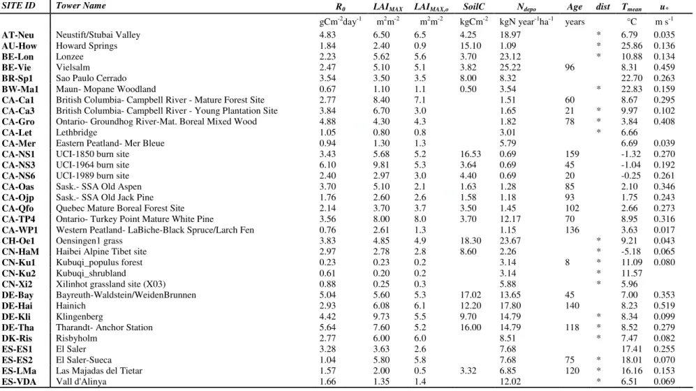
The data used in this analysis is based on the dataset from the FLUXNET (www.fluxdata.org) 187

eddy covariance network (Baldocchi, 2008, Baldocchi et al., 2001). The analysis was restricted to 188

104 sites (cf. Table in Appendix I and II) on the basis of the ancillary data availability (i.e. only 189

sites containing at least both leaf area index (LAI) of understorey and overstorey were selected) and 190

of the time series length (all sites containing at least one year of carbon fluxes and meteorological 191

data of good quality data were used). Further, we only analyzed those sites for which the relative 192

standard error of the estimates of the model parameters E0 (activation energy) and reference 193

respiration (R0) (please see further sections for more details on the meaning of parameters) were 194

less than 50% and where E0 estimates were within an acceptable range (0–450 K). 195

The latitude spans from 71.32° at the Alaska Barrow site (US-Brw) to -21.62° at the Sao Paulo 196

Cerrado (BR-Sp1). The climatic regions include tropical to arctic. 197

All the main PFTs as defined by the IGBP (International Geosphere-Biosphere Programme) 198

were included in this study: the selected sites included 28 evergreen needleleaf forests (ENF), 17 199 3 4 5 6 7 8 9 10 11 12 13 14 15 16 17 18 19 20 21 22 23 24 25 26 27 28 29 30 31 32 33 34 35 36 37 38 39 40 41 42 43 44 45 46 47 48 49 50 51 52 53 54 55 56 57 58 59 60

For Review Only

7

deciduous broadleaf forests (DBF), 16 grasslands (GRA), 11 croplands (CRO), 8 mixed forests 200

(MF), 5 savannas (SAV), 9 shrublands (SHB), 7 evergreen broadleaved forests (EBF) and 3 201

wetlands (WET). Due to limited number of sites and their similarity, the class SAV included both 202

the sites classified as savanna (SAV) and woody savannas (WSA), while the class SHB included 203

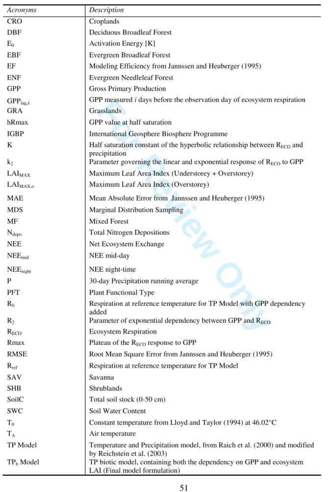
both the open (OSH) and closed (CSH) shrubland sites. For abbreviations and symbols refer to 204

Appendix III. 205

Daily RECO, GPP and the associated uncertainties of NEE data, together with daily 206

meteorological data such as mean air temperature (TA) and 30-day precipitation running average 207

(P), were downloaded from the FLUXNET database. 208

At each site data are storage corrected, spike filtered, u*-filtered according to Papale et al. (2006) 209

and subsequently gap-filled and partitioned as described by Reichstein et al. (2005). Only days 210

containing both meteorological and daily flux data with a percentage of gap-filled half hours below 211

15% were used for this analysis. The median of the u* threshold applied in the FLUXNET database 212

for the site-years used in the analysis are listed in the Appendix II. The average of the median u* 213

values are lower for short canopies (e.g. for grasslands 0.075±0.047 ms-1) and higher for tall 214

canopies (e.g. for evergreen needleleaf forests 0.221 ±0.115 ms-1). 215

Along with fluxes and meteorological data, main ancillary data such as maximum ecosystem 216

LAI (overstory and understory for forest sites) (LAIMAX), LAI of overstory (LAIMAX,o), stand age 217

for forests (StandAge), total soil carbon stock (SoilC) and the main information about disturbance 218

(date of cuts, harvesting) were also downloaded from the database. Total atmospheric nitrogen 219

deposition (Ndepo) is based on the atmospheric chemistry transport model TM3 (Rodhe et al., 2002) 220

and calculated at 1°x1° resolution. These data are grid-average downward deposition velocities and 221

do not account for vegetation effects. The data used for the selected sites are shown in the Appendix 222

II. 223 224

Development of the ecosystem respiration model 225

226

Site-by-site analysis – TP Model description

227 228

For the analysis of RECO we started from a widely used climate-driven model: ‘TP Model’ (Eq. 1) 229

proposed by Raich et al. (2002) and further modified by (Reichstein et al., 2003a). Here we used the 230

‘TP Model’ for the simulation of RECO at the daily time-step using as abiotic drivers daily TA and P: 231 232 ) ( ) (T f P f R R_ECO = _ref ⋅ _A ⋅ (1) 233 3 4 5 6 7 8 9 10 11 12 13 14 15 16 17 18 19 20 21 22 23 24 25 26 27 28 29 30 31 32 33 34 35 36 37 38 39 40 41 42 43 44 45 46 47 48 49 50 51 52 53 54 55 56 57 58 59 60

For Review Only

8 234

where Rref (gC m-2day-1) is the ecosystem respiration at the reference temperature (Tref, K) 235

without water limitations. f(TA) and f(P) are functional responses of RECO to air temperature and 236

precipitation, respectively. 237

Here temperature dependency f(TA) is changed from the Q10 model to an Arrhenius type equation 238

(Eq. 2). E0 (K) is the activation energy parameter and represents the ecosystem respiration 239

sensitivity to temperature, Tref is fixed at 288.15 K (15°C) and T0 is fixed at 227.13 K (-46.02°C): 240 241         − − − = 0 0 0 1 1 ) ( T T T T E A A ref e T f (2) 242 243

We refine the approach of Reichstein et al. (2003) and propose a reformulation of the response 244

of RECO to precipitation (Eq. 3), where k (mm) is the half saturation constant of the hyperbolic 245

relationship and α is the response of RECO to null P. 246 247

(

)

(

)

Although soil water content is widely recognized as the best descriptor of soil water availability, 250

we preferred to use precipitation since the model developed is oriented to up-scaling and soil water 251

maps are more affected by uncertainty than precipitation maps. 252

The model parameters – RREF, E0, α, k - were estimated for each site in order to evaluate the 253

accuracy of the climate-driven model. At each site the Pearson’s correlation coefficient (r) between 254

‘TP Model’ residuals (RECO observed minus RECO modelled ) and GPP was also computed. 255

256

Site-by-site analysis - Effect of productivity on the temporal variability of RECO 257

258

The role of GPP, as an additional biotic driver of RECO that has been included into Eq. 1, was 259

analysed at each site using three different formulations of the dependency of ecosystem respiration 260 on productivity f(GPP): 261 Linear response: f(GPP)=k₂⋅GPP (4) 262 Exponential response:

(

)

For Review Only

9

Beside the linear dependency the exponential and Michaelis-Menten responses were tested. 265

According to different authors (e.g. Hibbard et al., 2005, Reichstein et al., 2007) we hypothesized 266

that respiration might saturate at high productivity rates in a similar way to the Michaelis-Menten 267

enzyme kinetics. This saturation can also occur by a transition of carbon limitation to other 268

limitations. The exponential curve was used as another formulation of a saturation effect. 269

We tested two different schemes for the inclusion of f(GPP) (Eqs. 4, 5, 6) in the ‘TP Model’ 270

(Eq.1): 271

272

1) f(GPP) was included by replacing the reference respiration at reference temperature 273

(Rref in Eq. 1)with the sum of a new reference respiration (R0) and the f(GPP): 274

(

)

2) f(GPP) was included as an additive effect into the ‘TP Model’. In this case one part 276

of ecosystem respiration is purely driven by biotic factors (e.g. independent from 277

temperature) and the other one by abiotic ones. 278

279

In Table 1, R0 is the new reference respiration term (i.e. ecosystem respiration at Tref, when the 280

GPP is null and the ecosystem is well watered). This quantity is considered to be an indicator of the 281

ecosystem respiration of the site, strictly related to site conditions, history and characteristics, while 282

k2, R2, Rmax and hRmax describe the assumed functional response to GPP. 283

284

[TABLE1] 285

286

The model parameters - R0, E0, α, k and the parameters of ƒ(GPP) - were estimated for each site 287

in order to evaluate which model formulation best describes the temporal variability of RECO. 288

With the aim of confirming the existence of a time lag between photosynthesis and the 289

respiration response we ran the model with different time lagged GPP time-series (GPPlag,i), starting 290

from the GPP estimated on the same day (GPPlag,0), and considering daily increments back to GPP 291

estimated one week before the measured RECO (GPPlag,7). 292

GPP and RECO estimated with the partitioning method used in the FLUXNET database are 293

derived from the same data (i.e. GPP=RECO-NEE) and this may to some extent introduce spurious 294

correlation between these two variables. In literature two different positions on that can be found: 295

Vickers et al., (2009) argue that there is a spurious correlation between GPP and RECO when these 296

component fluxes are jointly estimated from the measured NEE (i.e. as estimated in the FLUXNET 297

database). Lasslop et al., 2009 demonstrated that, when using daily sums or further aggregated data, 298 3 4 5 6 7 8 9 10 11 12 13 14 15 16 17 18 19 20 21 22 23 24 25 26 27 28 29 30 31 32 33 34 35 36 37 38 39 40 41 42 43 44 45 46 47 48 49 50 51 52 53 54 55 56 57 58 59 60

For Review Only

10

self-correlation is important because of the error in RECO rather than because RECO being a shared 299

variable for the calculation of GPP. 300

Lasslop et al., 2010 further suggested a ‘quasi’-independent GPP and RECO estimates (GPPLASS 301

and RECO-LASS). The method by Lasslop et al., (2010) do not compute GPP as a difference, but 302

derive RECO and GPP from quasi-disjoint NEE data subsets. Hence, if existing, spurious correlations 303

is minimized. 304

To understand whether our results are affected or not by the ‘spurious’ correlation between GPP 305

and RECO estimated in FLUXNET, we also performed the analysis using the GPP and RECO 306

estimated by the partitioning method of Lasslop et al., (2010). The details of the analysis are 307

described in the Appendix IV. The results obtained confirmed (Appendix IV) that the data 308

presented and discussed in follow are not influenced by the possible ‘spurious’ correlation between 309

RECO and GPP reported in the FLUXNET data set. 310

311

Site-by-site analysis – Spatial variability of reference respiration (R0) 312

313

Once the best model formulation was defined, we analyzed the site-by-site (i.e. spatial) 314

variability of R0: the relationships between the estimated R0 at each site and site-specific ancillary 315

data were tested, including LAIMAX, LAIMAX,o , Ndepo, SoilC and Age. Leaf mass per unit area and 316

aboveground biomass were not considered because these are rarely reported in the database for the 317

sites studied and poorly correlated with spatial variability of soil respiration, as reported by 318

Reichstein et al. (2003a). In this analysis the sites with incomplete site characteristics were removed 319

(Age was considered only for the analysis of forest ecosystems). On the basis of this analysis the 320

model was reformulated by adding the explicit dependency of R0 on the site characteristics that best 321

explained its variability. 322

323

PFT–Analysis

324 325

In this phase we tried to generalize the model parameters in order to obtain a parameterization 326

useful for diagnostic PFT-based up-scaling. For this reason model parameters were estimated 327

including all the sites for each PFT at the same time. The dependency of R0 was prescribed as a 328

function of site characteristics that best explain the spatial R0 variability within each PFT class. 329

The model was corroborated with two different cross-validation methods: 330 331 3 4 5 6 7 8 9 10 11 12 13 14 15 16 17 18 19 20 21 22 23 24 25 26 27 28 29 30 31 32 33 34 35 36 37 38 39 40 41 42 43 44 45 46 47 48 49 50 51 52 53 54 55 56 57 58 59 60

For Review Only

11

1) Training/evaluation splitting cross-validation: one site at a time was excluded using the 332

remaining subset as the training set and the excluded one as the validation set. The model 333

was fitted against each training set and the resulting parameterization was used to predict the 334

RECO of the excluded site. 335

2) k-fold cross-validation: the whole data set for each PFT was divided into k randomly 336

selected subsets (k=15) called a fold. The model is fitted against k-1 remaining folds 337

(training set) while the excluded fold (validation set) was used for model evaluation. The 338

cross-validation process was then repeated k times, with each of the k folds used exactly 339

once as the validation set. 340

341

For each validation set of the cross-validated model statistics were calculated (see ‘Statistical 342

Analysis’ section). Finally, for each PFT we averaged the cross-validated statistics to produce a 343

single estimation of model accuracy in prediction. 344

345

Statistical analysis 346

347

Model parameters estimates

348 349

Model parameters were estimated using the Levenberg-Marquardt method, implemented in the 350

data analysis package “PV-WAVE 8.5 advantage” (Visual Numerics, 2005), a non-linear regression 351

analysis that optimize model parameters finding the minimum of a defined cost function. The cost 352

function used here is the sum of squared residuals weighted for the uncertainty of the observation 353

(e.g. Richardson et al., 2005). The uncertainty used here is an an estimate of the random error 354

associated with the night-time fluxes (from which RECO is derived). 355

Model parameter standard errors were estimated using a bootstrapping algorithm with N=500 356

random re-sampling with replacement of the dataset. As described by Efron and Tibshirani (1993), 357

the distribution of parameter estimates obtained provided an estimate of the distribution of the true 358

model parameters. 359

360

Best model formulation selection

361 362

For the selection of the ‘best’ model from among the six different formulations listed in Table 1 363

and the ‘TP Model’ we used the approach of the information criterion developed by Akaike (1973) 364

which is considered a useful metric for model selection (Anderson et al., 2000, Richardson et al., 365 3 4 5 6 7 8 9 10 11 12 13 14 15 16 17 18 19 20 21 22 23 24 25 26 27 28 29 30 31 32 33 34 35 36 37 38 39 40 41 42 43 44 45 46 47 48 49 50 51 52 53 54 55 56 57 58 59 60

For Review Only

12

2006). In this study the Consistent Akaike Information Criterion (cAIC, eq. 8) was preferred to the 366

AIC because the latter is biased with large datasets (Shono, 2005) tending to select more 367

complicated models (e.g. many explanatory variables exist in regression analysis): 368 369

( )

[

( )

]

where L(Θ) is the within samples residual sum of squares, p is the number of unknown parameters 372

and n is the number of data (i.e. sample size). Essentially, when the dimension of the data set is 373

fixed, cAIC is a measure of the trade-off between the goodness of fit (model explanatory power) 374

and model complexity (number of parameters), thus cAIC selects against models with an excessive 375

number of parameters. Given a data set, several competing models (e.g different model 376

formulations proposed in Table 1) can be ranked according to their cAIC, with the formulation 377

having the lowest cAIC being considered the best according to this approach. 378

For the selection of the best set of predictive variables of R0 we used the stepwise AIC, a 379

multiple regression method for variable selection based on the AIC criterion (Venables & Ripley, 380

2002, Yamashita et al., 2007). The stepwise AIC was preferred to other stepwise methods for 381

variable selection since can be applied to non normally distributed data (Yamashita et al., 2007). 382

383

Evaluation of model accuracy

384 385

Model accuracy was evaluated by means of different statistics according to Janssen and 386

Heuberger (1995): RMSE (Root Mean Square Error), EF (modelling efficiency), determination 387

coefficient (r2) and MAE (Mean Absolute Error). In particular EF is a measure of the coincidence 388

between observed and modelled data and it is sensitive to systematic deviation between model and 389

observations. EF can range from −∞ to 1. An EF of 1 corresponds to a perfect agreement between 390

model and observation. An EF of 0 (EF = 0) indicates that the model is as accurate as the mean of 391

the observed data, whereas a negative EF means that observed mean is a better predictor than the 392

model. In the PFT-analysis for each validation set the cross-validated statistics were calculated. The 393

average of cross-validated statistics were calculated for each PFT both for the training/evaluation 394

splitting (EFcv, RMSEcv, r2cv) and for the k-fold cross-validation (EFkfold-cv, RMSEkfold-cv, r2kfold-cv). 395 3 4 5 6 7 8 9 10 11 12 13 14 15 16 17 18 19 20 21 22 23 24 25 26 27 28 29 30 31 32 33 34 35 36 37 38 39 40 41 42 43 44 45 46 47 48 49 50 51 52 53 54 55 56 57 58 59 60

For Review Only

Results

The RMSE and EF obtained with ‘TP Model’ fitting (Table 2) showed a within-PFT-average EF 403

ranging from 0.38 for SAV to 0.71 for ENF and an RMSE ranging from 0.67 for SHB to 1.55 gC 404 m-2 d-1 for CRO. 405 406 [TABLE 2] 407 408

The importance of productivity is highlighted by residual analysis. A significant positive 409

correlation between the ‘TP Model’ residuals (z) and the GPP was observed with a systematic 410

underestimation of respiration when the photosynthesis (i.e. GPP) was intense. 411

In Fig. 1a, the mean r between the residuals and GPP for each PFT as a function of the time lag 412

is summarised. 413

The lowest correlation was observed for wetlands (r=0.29±0.14). The mean r is higher for 414

herbaceous ecosystems such as grasslands and croplands (0.55±0.11 and 0.63±0.18, respectively) 415

than for forest ecosystems (ENF, DBF, MF, EBF) which behaved in the same way (Fig. 1a), with a 416

r ranging from 0.35±0.13 for ENF to 0.45±0.13 for EBF. No time lag was observed with the

417

residuals analysis. 418

419

Gross Primary Production as driver of RECO 420

421

The effect of GPP as an additional driver of RECO was analyzed at each site by testing 6 different 422

models with the three different functional responses (Eqs. 4, 5 and 6) of respiration to GPP (Tab. 1). 423

The model ranking based on the cAIC calculated for each different model formulation at each site 424

showed agreement in considering the models using the linear dependency of RECO on GPP 425

(‘LinGPP’) as the best model formulation (Tab. 2), since the cAICs obtained with ‘LinGPP’ were 426

lower than those obtained with all the other formulations. This model ranking was also maintained 427

when analysing each PFT separately, except for croplands in which the ‘addLinGPP’ formulation 428

provided the minimum cAIC although the difference between the average cAIC estimated for the 429 3 4 5 6 7 8 9 10 11 12 13 14 15 16 17 18 19 20 21 22 23 24 25 26 27 28 29 30 31 32 33 34 35 36 37 38 39 40 41 42 43 44 45 46 47 48 49 50 51 52 53 54 55 56 57 58 59 60

For Review Only

14

two model formulations was almost negligible (cAIC was 38.22 ± 2.52 and 38.26 ± 2.45 for 430

‘addLinGPP’ and ‘LinGPP’, respectively) and the standard errors of parameter estimates were 431

lower for the ‘LinGPP’ formulation. In general, the cAIC obtained at all sites with the ‘LinGPP’ 432

model formulation (39.50 [37.50 – 42.22], in squared parentheses the first and third quartile are 433

reported)were lower than the ones obtained with the ‘TP Model’ (41.08 [39.02 - 44.40]), although the 434

complexity of the latter is lower (one parameter less). On this basis we considered the ‘LinGPP’ as 435

the best one model formulation. 436

The statistics of model fitting obtained with the ‘LinGPP’ model formulation are reported in 437

Table 2. The model optimized site by site showed a within-PFT-average of EF between 0.58 for 438

EBF to 0.85 for WET with an RMSE ranging from 0.53 for SAV to 1.01 gC m-2 day-1 for CRO. On 439

average EF was higher than 0.65 for all the PFTs except for EBF. In terms of improvement of 440

statistics, the use of ‘LinGPP’ in the ‘TP Model’ led to a reduction of the RMSE from 13.4 % for 441

shrublands to almost one third for croplands (34.8%), grasslands (32.5%) and savanna (32.0%) with 442

respect to the statistics corresponding to the purely climate driven ‘TP Model’. 443

444

[FIGURE 1] 445

446

No time lag between photosynthesis and respiration response was detected. In fact using GPPlag,-i 447

as a model driver we observed a general decrease in mean model performances for each PFT (i.e. 448

decrease of EF and increase of RMSE) for increasing i values (i.e. number of days in which the 449

GPP was observed before the observed RECO). The only exception were DBFs in which we found a 450

time lag between the GPP and RECO response of 3 days as shown by the peak in average EF and by 451

the minimum in RMSE in Fig. 1b, although the differences were not statistically significant. 452

453

Spatial variability of reference respiration rates

454 455

The reference respiration rates (R0) estimated site by site with the ‘LinGPP’ model formulation 456

represent the daily ecosystem respiration at each the site at a given temperature (i.e. 15°C), without 457

water limitation and carbon assimilation. Hence, R0 can be consider the respiratory potential of a 458

particular site. R0 assumed highest values for the ENF (3.01±1.35 gC m-2 day-1) while the lowest 459

values were found for SHB (1.49±0.82 gC m-2 day-1) and WET (1.11 ±0.17 gC m-2 day-1), possibly 460

reflecting lower carbon pools for shrublands or lower decomposition rates due to anoxic conditions 461

or carbon stabilization for wetlands. 462 3 4 5 6 7 8 9 10 11 12 13 14 15 16 17 18 19 20 21 22 23 24 25 26 27 28 29 30 31 32 33 34 35 36 37 38 39 40 41 42 43 44 45 46 47 48 49 50 51 52 53 54 55 56 57 58 59 60

For Review Only

15

By testing the pairwise relationship between R0 and different site characteristics we found that 463

the ecosystem LAIMAX showed the closest correlation with R0 (R0=0.44(0.04)LAIMAX+0.78(0.18), 464

r2=0.52, p<0.001, n=104, in parentheses standard errors of model parameters estimates were 465

reported), thus LAIMAX was the best explanatory variable of the retrieved R0 variability (Fig 2a). 466

Conversely, LAIMAX,o correlated weakly (r2=0.40, p<0.001, n=104) with R0 (Fig. 2b) indicating 467

that, for forest sites, understorey LAI must be also taken into account. A very weak correlation was 468

found with SoilC (r2=0.09; p<0.001, n=67) and no significant correlation with Age, Ndepo and 469

TMEAN were found for forest sites (Fig. 2 c-f). 470

471

[FIGURE 2] 472

473

The multiple regression analysis conducted with the stepwise AIC method including 474

simultaneously all sites, showed that the two best predictors of R0 were LAIMAX and SoilC 475

(Multiple r2=0.57; p<0.001; n=68) which were both positively correlated with R0 (Tab. 3). LAIMAX 476

was the best predictor of spatial variability of R0 for all sites confirming the results of the pairwise 477

regression analysis above mentioned but the linear model which included the SoilC as additional 478

predictor led to a significant, though small, reduction in the AIC during the stepwise procedure. 479

Considering only the undisturbed temperate and boreal forest sites (ENF, DBF, MF), the 480

predictive variables of R0 selected were LAIMAX and Ndepo. (Multiple r2=0.67; p<0.001; n=23). For 481

these sites both LAIMAX, which was still the main predictor of spatial variability of R0, and Ndepo 482

controlled the spatial variability of R0, with Ndepo negatively correlated to R0 (Tab. 3). This means 483

that for these sites, once removed the effect of LAIMAX, Ndepo showed a negative control on R0 with 484

a reduction of 0.025 gC m-2 day-1 in reference respiration for an increase of 1 kg N ha-1year-1. 485

Considering only the disturbed forest sites we found that SoilC and TMEAN were the best predictors 486

of spatial variability of R0 (Multiple R2= 0.80, p<0.001, n=10). 487

In Table 5 (left column) the statistics of the pairwise regression analysis between R0 and LAIMAX 488

for each PFT are reported. The best fitting was obtained with the linear relationship for all PFTs 489

except for deciduous forests for which the best fitting was obtained with the exponential 490

relationship R0=RLAI=0(1-e-aLAI). 491

492

[TABLE 3 AND TABLE 4] 493 494 PFT-Analysis 495 496 3 4 5 6 7 8 9 10 11 12 13 14 15 16 17 18 19 20 21 22 23 24 25 26 27 28 29 30 31 32 33 34 35 36 37 38 39 40 41 42 43 44 45 46 47 48 49 50 51 52 53 54 55 56 57 58 59 60

For Review Only

16

Final formulation of the model

497 498

On the basis of the aforementioned results, the GPP as well as the linear dependency between R0 499

and LAIMAX were included into the ‘TP Model’ leading to a new model formulation (Eq 9). The 500

final formulation is basically the ‘TP Model’ with the addition of biotic drivers (daily GPP and 501

LAIMAX) and hereafter referred to as ‘TPGPP-LAI Model’, where the suffixes GPP and LAI reflect 502

the inclusion of the biotic drivers in the climate-driven model: 503 504

(

)

(

)

where the term, RLAI=0 + aLAI LAIMAX, describes the dependency of the basal rate of respiration (R0 507

in Table1) on site maximum seasonal ecosystem LAI. Although we found that SoilC and Ndepo may 508

help to explain the spatial variability of R0, in the final model formulation we included only the 509

LAIMAX. In fact the model is primarily oriented to the up-scaling and spatial distributed information 510

of SoilC, Ndepo and disturbance may be difficult to be gathered and usually are affected by high 511

uncertainty. 512

The parameters RLAI=0 and aLAI listed in Table 4 were introduced as fixed parameters in the 513

‘TPGPP-LAI Model’. For wetlands and mixed forests the overall relationship between LAIMAX and 514

R0 was used. For wetlands, available sites were insufficient to construct a statistically significant 515

relationship while for mixed forests the relationship was not significant (p=0.146). 516

PFT specific model parameters (k2, E0, k, α) of ‘TPGPP-LAI Model’ were then derived using all 517

data from each PFT contemporarily and listed with their relative standard errors in Table 4. No 518

significant differences in parameter values were found when estimating all the parameters 519

simultaneously (aLAI, RLAI=0, k2, E0, k, α). 520

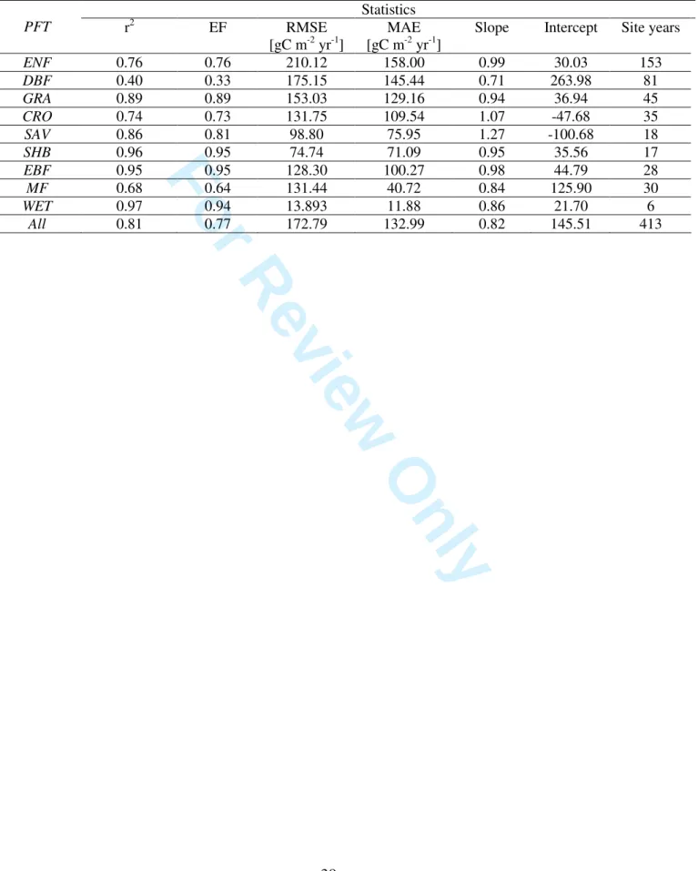
The scatterplots of the observed vs modelled annual sums of RECO are shown in Figure 3, while 521

results and statistics are summarized in Table 5. The model was well able to describe the 522

interannual and intersite variability of the annual sums over different PFTs, with the explained 523

variance varying between 40% for deciduous forests and 97% for shrublands and evergreen 524

broadleaved forests. Considering all sites, the explained variance is 81%, with a mean error of about 525

17% (132.99 gCm-2yr-1) of the annual observed RECO. 526 527 [TABLE 5, FIGURE 3] 528 3 4 5 6 7 8 9 10 11 12 13 14 15 16 17 18 19 20 21 22 23 24 25 26 27 28 29 30 31 32 33 34 35 36 37 38 39 40 41 42 43 44 45 46 47 48 49 50 51 52 53 54 55 56 57 58 59 60

For Review Only

17 529

Evaluation of model predictions accuracy and weak points

530 531

The results obtained with the k-fold and training/evaluation split cross-validation are listed in 532 Table 6. 533 534 [TABLE 6] 535 536

The r2cv ranges from 0.52 (for EBF) to 0.80 (for CRO) while the r2cv,kfold ranges from 0.58 (for 537

DBF) to 0.81 (for GRA). The cross-validated statistics averaged for each PFTare always higher for 538

the k-fold than for the training/evaluation splitting cross-validation. 539

The analysis of model residuals time series of the deciduous broadleaf forest (Fig. 4) showed a 540

systematic underestimation during the springtime development phase and, although less clear, on 541

the days immediately after leaf-fall. A similar behaviour was also found for croplands and 542

grasslands during the days after harvesting or cuts (Fig. 5). 543 544 [FIGURE 4,5] 545 546 DISCUSSION 547 548

Gross primary production as driver of ecosystem respiration 549

550

The results obtained with the purely climate-driven model (‘TP Model’) and the best model 551

formulation selected in the site-by-site analysis (i.e. ‘LinGPP’, Tab. 1) confirm the strong 552

relationship between carbon assimilation and RECO highlighting that this relationship must to be 553

included into models aimed to simulate temporal variability of RECO. 554

Respiration appears to be strongly driven by the GPP in particular in grasslands, savannas and 555

croplands as already pointed out by several authors in site-level analysis (Bahn et al., 2008, Moyano 556

et al., 2007, Wohlfahrt et al., 2008a, Xu & Baldocchi, 2004). For croplands and grasslands growth

557

respiration is controlled by the amount of photosynthates available and mycorrhizal respiration, 558

which generally constitutes a large component of soil respiration (e.g. Moyano et al., 2007, 559

Kuzyakov & Cheng, 2001). 560

For wetlands instead the weak relationship between respiration and GPP can be explained by the 561

persistence of anaerobic conditions, decomposition proceeds more slowly with an accumulation of 562 3 4 5 6 7 8 9 10 11 12 13 14 15 16 17 18 19 20 21 22 23 24 25 26 27 28 29 30 31 32 33 34 35 36 37 38 39 40 41 42 43 44 45 46 47 48 49 50 51 52 53 54 55 56 57 58 59 60

For Review Only

18

organic matter on top of the mineral soil layer and respiration is closely related to temperature and 563

water table depth rather than to other factors (Lloyd, 2006). 564

The lower correlation observed for forest ecosystems than for grasslands and croplands may be 565

due to the higher time for translocation, in trees, of substrates from canopy to roots, related to the 566

rates of phloem carbon transport (Nobel, 2005), which affect the reactivity of the respiration and the 567

release of exudates or assimilates from roots as response to productivity (Mencuccini & Höltta, 568

2010). This is very often cause of time lags between photosynthesis and respiration response but 569

may justify the reduction of correlation between model residuals and GPP estimated at the same 570

day. 571

A clear time lag between GPP and RECO response was not detected. In fact both the residual 572

analysis (Fig. 1a) and the analysis conducted with the ‘LinGPP’ model formulation (Fig. 1b) 573

confirmed the general absence of a time lag with the only exception of DBF where a time lag of 3 574

days was observed although the results were not statistically significant. However, in our opinion, 575

these results do not help to confirm or reject the existence of a time lag for several reasons: i) in 576

some studies (e.g. Baldocchi et al., 2006, Tang & Baldocchi, 2005) a lag on the sub-daily time scale 577

was identified and the lags on the daily time scale were attributed to an autocorrelation in weather 578

patterns (i.e. cyclic passage of weather fronts with cycles in temperature or dry and humid air 579

masses) which modulates the photosynthetic activities, since our analysis focused on daily data we 580

were not able to identify the existence of sub-daily time lags; ii) lag effects may be more 581

pronounced under favorable growing conditions or during certain periods of the growing season, the 582

analysis of which analysis is out of scope of present study. 583

584

Spatial variability of reference respiration rates

585 586

The relationship between reference respiration rates (R0) derived by using the ‘LinGPP’ model 587

formulation, and LAIMAX (Fig. 2a) is particularly interesting considering that the productivity was 588

already included into the model (i.e. daily GPP is driver of ‘LinGPP'). While daily GPP describes 589

the portion of RECO that originates from recently assimilated carbon (i.e. root/rhizosphere 590

respiration, mychorrizal and growth respiration), LAIMAX is a structural factor which has an 591

additional effect to the short-term productivity and allows to describe the overall ecosystem 592

respiration potential of the ecosystem. For instance, high LAI means increased autotrophic 593

maintenance respiration costs. Moreover LAIMAX can be considered both as an indicator of the 594

general carbon assimilation potentialand as an indicator of how much carbon can be released to soil 595

yearly because of litterfall (in particular for forests) and leaf turnover which are directly related to 596 3 4 5 6 7 8 9 10 11 12 13 14 15 16 17 18 19 20 21 22 23 24 25 26 27 28 29 30 31 32 33 34 35 36 37 38 39 40 41 42 43 44 45 46 47 48 49 50 51 52 53 54 55 56 57 58 59 60

For Review Only

19

basal soil respiration (Moyano et al., 2007). At recently disturbed sites, this equilibrium between 597

LAIMAX and soil carbon (through litter inputs) may be broken, for example thinning might lead to a 598

reduction of LAIMAX without any short-term effect on the amount soil carbon, while ploughing in 599

crops or plantations leads solely to a reduction in soil carbon content and not necessarily in LAI. 600

Also in cut or grazed grasslands maximum LAI does not correspond well with litter input because 601

most of this carbon is exported from the site and only partially imported back (as organic manure). 602

This explains why the multiple linear model including LAIMAX and SoilC was selected as the best 603

by the stepwise AIC regression using all the sites contemporarily and why considering only 604

disturbed forest ecosystems we SoilC was selected as best predictor of R0 (Tab. 3). 605

Particularly interesting is also the negative control of Ndepo on R0 with a reduction of 0.025 gC m -606

2 _day-1 _{in R}

0 for an increase of 1 kg N ha-1year-1. The reduction of heterotrophic respiration in sites 607

with high total nitrogen deposition load was already described in literature and in some site-level 608

analysis and attributable to different processes. For instance soil acidification at high Ndepo loads 609

may inhibit litter decomposition suppressing the respiration rate (Freeman et al., 2004, Knorr et al., 610

2005) and increasing in Ndepo can increase N concentration in litter with a reduction of litter 611

decomposition rates (Berg & Matzner, 1997, Persson et al., 2000) and the consequent reduction of 612

respiration.The latter process is more debated in literature because increased N supply may lead to 613

higher N release from plant litter, which results in faster rates of N cycling and in a stimulation of 614

litter decomposition (e.g. Tietema et al., 1993). However this process is not always clear (e.g. Aerts 615

et al., 2006): in litter mixtures, N-rich and lignin-rich litter may chemically interact with the 616

formation of very decay-resistant complexes (Berg et al., 1993). In addition, litter with a high 617

concentration of condensed tannins may interact with N-rich litter reducing the N release from 618

decomposing litter as described in Hattenschwiler and Vitousek (2000). Thus, the supposed 619

stimulating effects of N addition on N mineralization from decomposing litter may be counteracted 620

by several processes occurring in litter between N and secondary compounds, leading to chemical 621

immobilization of the added N (e.g. Pastor et al., 1987, Vitousek & Hobbie, 2000) 622

Although the absolute values are a matter of recent debate (De Vries et al., 2008, Magnani et al., 623

2007, Sutton et al., 2008), it is agreed that Ndepo stimulates net carbon uptake by temperate and 624

boreal forests. As net carbon uptake is closely related to respiration, once the effect of age is 625

removed, it can be seen that increased Ndepo has the potential to drive RECO in either directions. The 626

stimulation of GPP as consequence of the increasing Ndepo is already include in the model since 627

GPP is a driver. Additionally our analysis suggests that overall an increased total Ndepo in forests 628

tends to reduce reference respiration. Without considering the effects introduced by Ndepo in our 629

models we may overestimate RECO, with a consequent underestimation of the carbon sink strength 630 3 4 5 6 7 8 9 10 11 12 13 14 15 16 17 18 19 20 21 22 23 24 25 26 27 28 29 30 31 32 33 34 35 36 37 38 39 40 41 42 43 44 45 46 47 48 49 50 51 52 53 54 55 56 57 58 59 60

For Review Only

20

of such terrestrial ecosystems. It is also clear that, in managed sites, such interactions apply equally 631

to other anthropogenic nitrogen inputs (fertilizers, animal excreta) (e.g. Galloway et al., 2008). 632

However, considering i) that LAIMAX is the most important predictor of R0, ii) that the uncertainty 633

in soil carbon and total nitrogen deposition maps is usually high, iii) that the spatial information on 634

disturbance is often lacking and finally iv) that our model formulation is oriented to up-scaling 635

issues, we introduced LAIMAX as the only robust predictor of the spatial variability of R0 in the final 636

model formulation. 637

The use of LAIMAX is interesting for an up-scaling perspective (e.g. at regional or global scale) 638

since can be derived by remotely sensed vegetation indexes (e.g. normalized vegetation indexes or 639

enhanced vegetation indexes) opening interesting perspectives for the assimilation of remote 640

sensing products into the ‘TPGPP-LAI Model’. 641

The intercepts of the PFT-based linear regression between R0 and LAIMAX (Tab.4) suggest that, 642

when the LAIMAX is close to 0 (‘ideally’ bare soil), the lowest R0 takes place in arid (EBF,SHB and 643

SAV) and agricultural ecosystems,. The frequent disturbances of agricultural soils (i.e. ploughing 644

and tillage), as well as management, reduce soil carbon content dramatically. In croplands, the 645

estimated R0 is very low in sites with low LAI. However, with increasing LAIMAX, R0 shows a rapid 646

increase, thus resulting in high respiration rates for crop sites with high LAI. For EBF, SHB and 647

SAV the retrieved slopes are typical of forest ecosystems, while the intercepts are close to zero 648

because of the lower soil carbon content usually found in these PFTs (Raich & Schlesinger, 1992). 649

Because of the few available sites representing and on similarity in terms of climatic characteristics, 650

savannas, shrublands were grouped. 651

In grasslands, the steeper slope (aLAI) value found (1.14 ± 0.33) suggests that R0 increases 652

rapidly with increasing aboveground biomass as already pointed out in literature (Wohlfahrt et al., 653

2008a, Wohlfahrt et al., 2005a, Wohlfahrt et al., 2005b), i.e. an increase in LAIMAX leads to a 654

stronger increase in R0 than in other PFTs. 655

In forest ecosystems, and in particular in evergreen needleleaf and deciduous broadleaf forests, 656

the physical meaning of the higher intercept may be found in less soil disturbance. In boreal forests, 657

the soil carbon stock is generally high even at sites with low LAIMAX, thus maintaining an overall 658

high R0 which is less dependent on the LAIMAX. 659

660

Final formulation of the model and weak points

661 662

These results obtained with the ‘TPGPP-LAI Model’ cross-validation indicate that the developed 663

model describes the RECO quite well. In particular results indicate a better description of the 664 3 4 5 6 7 8 9 10 11 12 13 14 15 16 17 18 19 20 21 22 23 24 25 26 27 28 29 30 31 32 33 34 35 36 37 38 39 40 41 42 43 44 45 46 47 48 49 50 51 52 53 54 55 56 57 58 59 60

For Review Only

21

temporal variability of RECO rather than the spatial variability (or across-site variability). In the 665

training/evaluation splitting in fact, the excluded site for each PFT is modelled using a 666

parameterization derived from the other sites within the same PFT. However, the k-fold is more 667

optimistic than training/evaluation splitting cross-validation because the data set is less disturbed 668

and the calibration and validation datasets are statistically more similar. In the training/evaluation 669

splitting, instead, we exclude one site which is completely unseen by the training optimization 670

procedure. 671

The derived parameterization of the ‘TPGPP-LAI Model’ reported in Table 4 may be considered 672

as an optimized parameterization for the application of the model at large scale (e.g. continental or 673

global). For this application is necessary to link of the developed model with a productivity model 674

and remote sensing products necessary for the estimation of LAI. One of the main advances 675

introduced by this model formulation is the incorporation of GPP and LAI as driver of the 676

ecosystem respiration, which importance in modeling Reco is above discussed. These variables are 677

necessary to improve the description of both the temporal and spatial dynamics or RECO. These 678

results imply that empirical models used with remote sensing (e.g. Reichstein et al., 2007, 679

Reichstein et al., 2003a, Veroustraete et al., 2002) underestimate the amplitude of RECO an might 680

lead to wrong conclusions regarding the interpretation of seasonal cycle of the global CO2 growth 681

rate and annual carbon balance. 682

The values of the ‘TPGPP-LAI Model’ parameters (Tab. 4) related to the precipitation (k, α) 683

indicated a much stronger nonlinearity in the response of RECO to precipitation for shrublands, 684

wetlands and croplands than for forest ecosystems (Fig. 6). Wetlands and croplands reached 685

saturation (no limitation of water on respiration) after a small rain event underlying their 686

insensitivity to precipitation owing to the presence of water in wetland soils and irrigation in 687

croplands. Grasslands are very sensitive to rain pulseas described in Xu & Baldocchi et al. (2004), 688

while savannas and evergreen broadleaved forests showed a strong limitation when rainfall was 689

scanty and f(P) saturation exceed 50 mm month-1. The parameters related to GPP dependency (k2) 690

estimated at PFT level confirm all the results obtained at site level indentifying a clear sensitivity of 691

grasslands and savannah to GPP. 692

[FIGURE 6] 693

However, when comparing these parameterizations, it is very likely that a background 694

correlation between precipitation, short-term productivity and soil respiration confused the apparent 695

response of respiration to water availability in the ‘TPGPP-LAI Model’. 696

Despite the good accuracy, some criticisms and limitations of the ‘TPGPP-LAI Model’ were 697

identified, in particular for the deciduous broadleaf forests. The systematic underestimation during 698 3 4 5 6 7 8 9 10 11 12 13 14 15 16 17 18 19 20 21 22 23 24 25 26 27 28 29 30 31 32 33 34 35 36 37 38 39 40 41 42 43 44 45 46 47 48 49 50 51 52 53 54 55 56 57 58 59 60