Ab-Initio Simulation of Novel Solid Electrolytes
by
William D. Richards
Submitted to the Department of Materials Science and Engineering
in partial fulfillment of the requirements for the degree of
Master of Science in Materials Science and Engineering
"
"""
MA SSACHUSETTS INSTM/tE.at the OF TECHNOLOGY
IMAY
14
2O14
MASSACHUSETTS INSTITUTE OF TECHNOLOGY!
February 2014
LIBRARIES
@
Massachusetts Institute of Technology 2014. All rights reserved.
Author ...
...
Department of Materials Science and Engineering
October 3, 2013
Certified by...
Gerbrand Ceder
R. P. Simmons Professor of Materials Science and Engineering
Thesis Supervisor
A ccepted by ...
...
Gerbrand Ceder
Chairman, Department Committee on Graduate Students
Ab-Initio Simulation of Novel Solid Electrolytes
by
William D. Richards
Submitted to the Department of Materials Science and Engineering on October 3, 2013, in partial fulfillment of the
requirements for the degree of
Master of Science in Materials Science and Engineering
Abstract
All solid-state batteries may be a solution to some of the problems facing conventional organic electrolytes in Li and Na-ion batteries, but typically conductivities are very low. Reports of fast lithium conduction in Lii0GeP 2S1 2 (LGPS), with conductivity
of 12 mS/cm at room temperature, have shown that Li -diffusion in solid electrolytes can match or exceed the liquid electrolytes in use today. I report results of ab-initio calculations on a related system of materials, Nai0MP 2SI2 (M = Ge, Si, Sn), which are predicted to have similar properties to LGPS as candidates for electrolytes in Na-ion batteries. I also derive methods to estimate the error associated with diffusNa-ion simulations, so that appropriate tradeoffs between computational time and simulation accuracy can be made. This is a key enabler of a high throughput computational search for new electrolyte materials.
Thesis Supervisor: Gerbrand Ceder
Acknowledgments
I would like to express my gratitude to my advisor, Professor Ceder, for introducing
me to this fascinating field, as well as his continuing genuine interest in all of the work of his students. Discussions with him seemingly always find a way to yield new insights into the problem at hand.
This work is of course made so much more enjoyable by the support from and exchange of ideas with such a talented research group. I especially thank Shyue Ping Ong and Yifei Mo, two postdocs who I joined on the project; none of this work would have been possible without close help from them.
And it goes almost without saying that the support of my friends and family who have encouraged and been there for me throughout this endeavor has been
Contents
1 Introduction 1.1 Intercalation batteries . . . . 1.1.1 L i-ion . . . . 1.1.2 N a-ion . . . . 1.1.3 E lectrolytes . . . . 1.2 Computational modeling . . . .1.2.1 Calculating diffusivity using computational simulation . . . . 1.3 Outline of this thesis . . . .
2 Nai0MP 2S12 (M = Ge, Si, Sn) solid electrolytes
2.1 The structure of NMPS . . . . 2.2 Phase stability . . . . 2.3 Cathodic and anodic stability . . . . 2.4 D iffusivity . . . . 2.5 C onclusions . . . .
3 Error bounds for diffusivity calculations
3.1 Diffusivity from the random walk . . . .
3.2 Distribution of measurements of mean squared displacements . . . . .
3.2.1 Relating the theoretical distribution to simulation observables
3.3 A credible interval for MSD . . . . 3.3.1 Choosing a prior distribution . . . .
13 14 14 14 15 16 16 18 19 20 22 23 24 27 29 30 32 33 34 35
3.4 Comparison of Bayesian credible intervals to the Frequentist confidence interval . . . . 37
List of Figures
2-1 Structures of LGPS determined from (a) Kamaya et al.[13] and (b) K uhn et al.[18] . . . . 20 2-2 Lowest DFT energy LGPS structure (P4m2 symmetry) . . . . 21
2-3 Lowest DFT energy structures of (a) NaSiPS, NaSnPS (C222 symme-try) and (b) NaGePS (P1 symmesymme-try) . . . . 22 2-4 Arrhenius plots for diffusivity of: (a) NaGePS, P1 symmetry (b) NaGePS,
C222 symmetry (c) NaSiPS (d) NaSnPS . . . . 26
3-1 Discrete MSD distributions with (a) nobs = 5, p = 3 (b) nobs =15, t = 3 33 3-2 (a) Single skellam variable + noise with p = 1 (b) MSD probability
distribution with no0b = 3, i 1 . . . . 34
3-3 Bounds as a function of MSD for various nobs: (a) upper bound with uniform prior (b) lower bound with log-uniform prior . . . . 37
3-4 Comparison of Bayesian upper bound with bounds based on Poisson and Chi squared distributions for nobs = 6 . . . . 39
List of Tables
2.1 Phase equilibria and decomposition energies for X1OMP 2S1 2. . . . . . 23 2.2 Phase equilibria for NaiOMP 2X12 composition at cathode and anode PgNa. 24
2.3 Ionic conductivity of cation-substituted compounds X1OMP 2S12 (X=Li,
Chapter 1
Introduction
Continued improvement of battery technology is required and in many cases the driving force for development in a wide range of applications, including consumer electronics, grid load-leveling and storage, and electric vehicles. The function of a battery is a simple one -energy is stored in a chemical potential difference between an anode and a cathode. This energy is harnessed by allowing charged ions to equilibrate across an electrolyte, creating an electrical potential across the electrodes. Recharging of the battery is accomplished by applying a larger voltage in the opposite direction, driving the reverse reaction. The simplicity of the battery puts great emphasis on the materials from which it is made - there are relatively few gains that can be made to the device besides directly improving component materials.
Battery performance is characterized by two main parameters - energy density (or specific energy) and rate capability. Energy density is a function of cell voltage (V) and charge capacity (mAh/g). The achievable discharge rate is determined by the electronic transport through the electrodes, and the ionic transport through the cathode and electrolyte. Improvements therefore come through increasing voltage, charge capacity, or rate capability.
1.1
Intercalation batteries
Early battery technologies, such as lead-acid, Ni-Cd, and Zn-MnO2, involve the
con-version of the electrode structure upon charge and discharge. One of the major breakthroughs in battery technology was the development of intercalation materials, which operate via insertion and deinsertion of ions into a host framework, the struc-ture of which is unchanged through cycling. The composition of the electrolyte is constant in these systems, as the working ion is shuttled between the two electrodes. This allows a much smaller amount of electrolyte to be used, as no ions are stored in the electrolyte. In these batteries, the working ion must diffuse quickly through the electrode materials, so these batteries are restricted highly mobile ions, such as Li+ and Na+.
1.1.1
Li-ion
Lithium ion batteries, first commercialized by Sony in 1991, make up an enormous fraction of the cells used in portable electronics today, and are in use in some electronic cars (e.g. Tesla). They typically operate via reversible intercalation of lithium ions between a graphite (LixC6) anode and a transition metal oxide (LilxMO2) cathode,
most typically with either cobalt, nickel or manganese (or some combination) as the transition metal. Another common cathode is LiFePO4, which has an olivine
structure. The average charge capacity (180 Wh/kg at 3.8V) is a factor of 5 higher than lead-acid batteries.
1.1.2
Na-ion
Despite the long history of development of sodium batteries dating to the 1960s, and their concurrent development with Li-ion, development of Na-ion batteries for a while stagnated due to their lower voltage and energy density compared with Li. The push for lower-cost materials has brought them back into relevance. Sodium occurs naturally with a significantly higher abundance than lithium, and cheaper redox active elements can be used; In Li-ion cells, the cobalt is a large expense.
While phase transformations in many layered Li-ion systems have been observed, their Na-ion counterparts are significantly more stable[16].
A major difference between the Li-ion and Na-ion systems is the choice of anode.
Sodium doesn't intercalate into graphite, and so other anode materials must be used, typically hard carbon, or titania[25]. Cathodes materials are similar between Li-ion and Na-ion systems, though many of the layered oxides that are not stable for Li-ion do not pose a problem in Na-ion batteries.
1.1.3
Electrolytes
In Li and Na-ion batteries, the choice of electrolyte is very important for device performance. Because the cell voltage exceeds 1.23V, aqueous electrolytes cannot be used without significantly reducing the operating voltage. Typically, the electrolyte is an alkyl carbonate such as ethylene carbonate (EC) or dimethyl carbonate (DMC) with LiPF6. These materials are only stable down to 1.5V vs. lithium metal, and
below this a solid-electrolyte-interphase (SEI) layer forms, partially passivating the surface[20]. They can also be oxidized by the cathodes when delithiated. This is especially an issue with high-voltage cathodes (e.g. LiNiO2) and so the use of organic
electrolytes puts an upper limit on the safe operating voltage. Similar problems are seen in Na-ion batteries.
The reactivity of electrolytes is a safety issue as well as a performance one. Organic solvents are flammable, and their proximity to an oxidizing agent (the cathode) can lead to thermal runaway, and in extreme cases fire or explosion. Though with careful engineering, this danger is effectively mitigated, a number of incidents over the years have resulted in product recalls[3].
Solid electrolytes have been proposed as a solution for some of these limitations.
A number of such materials have been known since the 1980s, though large
activa-tion energies have limited their use to high temperature systems, or those with very slow discharge rates. In 2011, Kamaya et al.[13] reported the discovery of a new Li superionic conductor Li10GeP2S12, which achieved a room temperature
large amount of germanium needed is expensive, and large resistances develop at the cathode interface.
1.2
Computational modeling
Computational models of materials are able to both aid in the understanding of existing materials, and to predict the structure and properties of as-yet unsynthesized novel compounds. Computational techniques have been used to great effect in the battery field to study electrode materials, and properties such as stability, capacity,
and even safety can be readily calculated[11, 30].
While it has been, in principle, possible to calculate ground state properties of ma-terials since the development of the Schrodinger equation, this problem has remained computationally intractable for all but the simplest of systems, due to the many in-teractions between every electron in the system. Density functional theory (DFT) provides a method of reducing the problem size such that it can tackle problems at
a size relevant to many more systems, including battery materials. It does this by avoiding calculating single particle orbitals, and instead treating the electrons as an electron gas and defining functionals for the electron-electron interaction energy, the kinetic energy and the exchange energy are defined as functions of its density[7].
Many of the properties relevant to cathode materials are also important for elec-trolytes. Additionally, it is critical that a solid electrolyte have high ionic conductivity. The calculation of material kinetics, while a more complex problem than equilibrium thermodynamics, can also be simulated computationally.
1.2.1
Calculating diffusivity using computational simulation
Depending on the particulars of the system involved, a number of methods are used to study diffusion computationally. These typically fall into categories of either using transition state theory and calculating attempt frequencies and activation energies, or simulating atomic motion explicitly in a molecular dynamics (MD) simulation and determining self diffusivity from atom trajectories. To combat the difficulties in
simulating the long timescales needed to observe diffusion in some systems, a number of methods for artificially accelerating transition events in MD have been developed.
Transition state theory/NEB
Diffusivity can be determined by calculation and integration of the individual dif-fusive mechanisms. This method is very similar to the calculation of reaction rates using transition state theory (TST) in that it involves the calculation of an activa-tion energy (E) and a kinetic prefactor associated with the attempt frequency and vibrational frequency. Typically, the nudged elastic band method (NEB) is used to calculate E,[12]. This method calculates the energy of the transition state by calcu-lating the energies of a series of images allowed to move perpendicular to the reaction path. To find the correct saddle point with fewer images, a climbing image can be used, which is allowed to move towards the saddle point
[9].
These methods allow relatively computationally cheap computation of diffusivity, though a large amount of information needs to be known about the system a priori. The diffusion path needs to be initialized with a reasonable guess, and since most cases of diffusion involve va-cancies or interstitials, the prevalence (and in many cases interaction) of these defects must be understood.Molecular dynamics
Molecular dynamics (MD) simulations simulate a material at finite temperature, tracking the position of atoms over time, calculating diffusivity from the trajectories. These simulations can be performed given any energy model by integrating Newton's equations of motion. Energies have been calculated using atomic potentials, either fit to experimental data, or to ab initio calculations. Due to its importance in hydrogen fuel cells, a large amount of literature is focused on the calculation of 02- diffusion in oxides[14, 15, 5]. Calculations on a range of solid electrolytes including argyrodite Li6PS5X (X = Cl, Br, I) and garnet Li7_,La3(Zr2-M,)O1 2 (M = Ta, Nb) have been performed utilizing a soft bond-valence approach[2, 1].
made simulation with forces directly calculated from DFT practicable for an increas-ing range of systems. These are typically systems with very high diffusivities, and include lithium diffusion in Li3N[28], and hydrogen diffusion in a-iron[27].
Accelerated MD/metadynamics
For systems where diffusivity is too slow to measure via an MD simulation (either ab initio or with an atomic potential), a number of methods have been devised to speed up sampling of diffusive transitions. These include hyperdynamics [29], which applies a bias potential to some aspects of the system and adjust the time scale accordingly, and metadynamics (or conformational flooding)[8], which explores free energy space
by sequentially applying bias potentials to on relevant collective variables to move
out of local minima. A comprehensive review of this class of methods is given by Dellago et al.[6].
1.3
Outline of this thesis
This thesis is part of ongoing work to find novel solid electrolytes. In this search, we are primarily concerned with materials with high diffusivity, though they span many different chemistries. For this reason, ab initio MD is the method of choice, since it requires no adaptation between chemical systems. The restriction of the search to high conductivity materials mitigates the downside of this method -its high computational cost.
Chapter 2 takes an in-depth look at sodium versions of the recently reported LGPS class of solid electrolytes, while chapter 3 uses a statistical approach to address the challenge of determining diffusivity from small amounts of MD data to allow a wider search space with a fixed computational budget.
Chapter 2
Na
1
OMP
2
S
1
2
(M
Ge, Si, Sn) solid
electrolytes
Since the first reports of high Li-ion conductivity in LiiOGeP2SI2 (LGPS), there have
been questions of whether similar materials exist. This is due to a few deficiencies of LGPS: While initially believed to be stable over a wide electrochemical window, computational studies [21] have shown that it is likely unstable against both the cathode and vs. lithium metal. Electrolyte reduction in contact with lithium metal has been observed experimentally[19], and high interfacial resistances at the cathode have also been observed, though the source of these is still not well understood. The use of significant amounts of germanium in the material is also an issue do to the high cost and low availability of the element.
Computational studies, being somewhat chemically agnostic, are a useful tool for answering these questions, as well as clarifying ambiguous experimental results. We examined the LiiOiiMP2X1 2 (M = Ge, Si, Sn, Al; X=O, S, Se) family of materials
isostructural to LGPS to identify promising new electrolytes[22], finding that cation substitutions can generally yield materials comparable to LGPS.
This chapter examines the feasibility of making the substitution of Na for Li to form the NaiOMP 2S12 (NMPS) system, and their suitability for use as electrolytes in
*Li
e
Os
(a) (b)
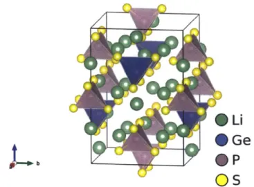
Figure 2-1: Structures of LGPS determined from (a) Kamaya et al.[13] and (b) Kuhn et al.[18]
2.1
The structure of NMPS
The structure of NaioMP2S12 (NMPS) used for this computational study is derived
from the experimentally determined structure of LGPS. The LGPS structure has tetragonal symmetry, and consists of (Geo.5Po.5)S4 tetrahedra, PS4 tetrahedra, LiS6
octahedra, and LiS4 tetrahedra. The LiS4 tetrahedra are arranged in a 1 dimensional
chain along the c-direction. The crystal structure obtained by Rietveld refinement is described in two works, the initial report of LGPS from Kamaya et al.
[13],
and in the results of single crystal XRD [18]. The structures are shown in figure 2-1. The main difference between the two is the presence of an additional lithium site (Li4) at fractional coordinates [0,0,0.25] in the more recent study.In both LGPS structures, there is a high degree of disorder both on the Li and P/Ge sites. In order to determine the ground state energy, the lowest energy order-ing must be found. As an initial approximation, the electrostatic energy was used to determine the lowest energy orderings, taking the idealized charges from the valence state, i.e. P5+, Ge4+ S2-, Li+. The lowest electrostatic energy configurations were
Ge
O s
Figure 2-2: Lowest DFT energy LGPS structure (P4m2 symmetry)
the pymatgen[23] open source software package. Ten of these low-energy configura-tions were calculated using DFT to determine the ground state. These calculaconfigura-tions were performed using the Vienna Ab Initio Simulation Package (VASP) [17] using the projector augmented-wave method[4]. Calculations used the Perdew-Burke-Ernzerhof generalized-gradient approximation (GGA) to density functional theory (DFT)[26].
All energy calculations were performed with k-point densities of at least 500/natoms
and were spin-polarized. The lowest DFT energy structure, shown in figure 2-2 main-tains much of the symmetry of the disordered structure, though the ordering of the P/Ge sites reduces the spacegroup to P4m2. Orderings of the Kamaya structure were all higher energy due to the lack of the low energy Li4 site.
To determine the correct sodium substituted structures, the low energy electro-static orderings for the LGPS structure were substituted with Na, and their energies computed using DFT. Since Li and Na have the same valence state, there is no differ-ence in the electrostatic orderings between the chemistries. The results of DFT cal-culations reveal a slight difference between the low energy Li1oMP2S1 2 structures and
the low energy Na1OMP 2S12 structures. In the Li system, all ground state structures
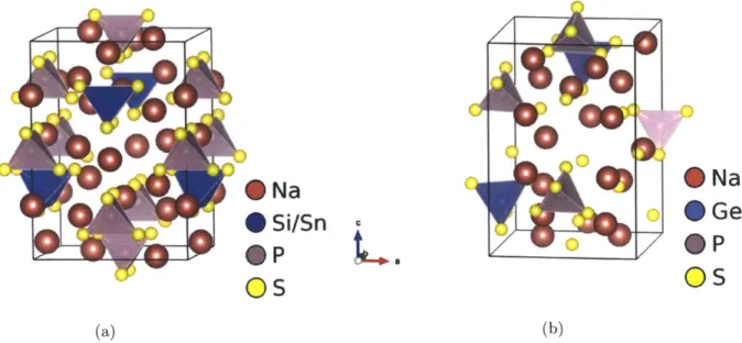
have P4m2 symmetry (figure 2-2). The Na1OSiP 2S12 and Na1oSnP2S12 structures have
L-10
(a)
Figure 2-3: Lowest DFT energy structures of and (b) NaGePS (P1 symmetry)
(b)
*Na
*Ge
ep
Os
(a) NaSiPS, NaSnPS (C222 symmetry)
ordering between the c-axis channels, which may be more favorable due to higher Na-Na repulsion than in the Li structure. In the Nai0GeP2S12 structure, the lowest
energy ordering was found to have P1 symmetry(figure 2-3b), but followed the trend of C222 symmetry being lower energy than P4m2 symmetry.
2.2
Phase stability
The most basic criterion for material stability is that there be little to no driving force for decomposition through phase separation, or by transforming to a lower energy structure at the same composition. The phase diagram, as well as this driving force for decomposition, can be determined by computing the lower convex hull of the structure energies in composition space. The driving force for decomposition is then the energy above the hull, which is typically referenced on a per atom basis.
Obtaining the stability of the structure requires calculating the energies of all neighboring phases in the phase diagram to ensure the correct convex hull at the structure composition. For this analysis, energies of all ICSD structures in the XMPS
chemical system, with X=Li, Na and M=Si, Ge, Sn were calculated, and from these, all stable Li containing structures were substituted with Na and also calculated. Additionally, all LixPySz structures compiled by Holzwarth et al.[10] were computed for both Li and Na.
Similar to our computational results on LGPS [21] and the LMPS system [22], NGPS is found to be slightly unstable at OK, but with a low energy above hull, so that it likely becomes entropically stabilized at moderate temperature due to the large amount of cation disorder. Comparison of the stability of the Li and Na substituted LGPS is given below in table 2.1.
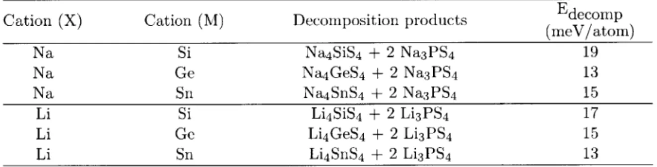
Table 2.1: Phase equilibria and decomposition energies for X10MP2S12.
Cation (X) Cation (M) Decomposition products Edecomp
(meV/atom) Na Si Na4SiS4 + 2 Na3PS4 19 Na Ge Na4GeS4 + 2 Na3PS4 13 Na Sn Na4SnS4 + 2 Na3PS4 15 Li Si Li4SiS4 + 2 Li3PS4 17 Li Ge Li4GeS4 + 2 Li3PS4 15 Li Sn Li4SnS4 + 2 Li3PS4 13
The difference in the LGPS stability between these data and Ong et al.[22] is due to the lower energy configuration found using the newer experimentally determined
LGPS structure[18] as the starting structure for electrostatic ordering.
2.3
Cathodic and anodic stability
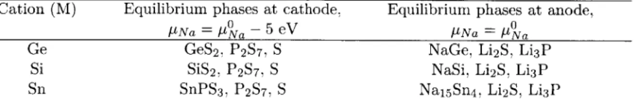
In addition to stability in isolation, an electrolyte material must retain its stability when in contact with the battery cathode and anode, which can act as lithium sources and sinks. To examine phase stability at these extremes, grand potential phase dia-grams were constructed following the procedure of Ong et al.[24]. From these phase diagrams, we determine the equilibrium phases at P4Na corresponding to bulk metallic sodium (anode) and (puNa - 5) eV corresponding to a 5V charged cathode. Results are summarized in table 2.2.
Table 2.2: Phase equilibria for Na1 0MP 2X1 2 composition at cathode and anode IptNa-Cation (M) Equilibrium phases at cathode, Equilibrium phases at anode,
0 0
pNa f1Na- 5 eV PNa pNa
Ge GeS2, P2S7, S NaGe, Li2S, Li3P
Si SiS2, P2S7, S NaSi, Li2S, Li3P
Sn SnPS3, P2S7, S Nai5Sn4., Li2S, Li3P
Unsurprisingly, the results are very similar to LMPS. When all of the alkali metal is removed from the system (at the cathode), the equilibrium phases are identical between LMPS and NMPS. At the anode, the reaction products are similar to LMPS, though the Na content in the resulting NaM. phases is lower.
2.4
Diffusivity
The ionic conductivity of an electrolyte is an important measure of its performance, as it contributes to the rate capability of the overall battery. Low electrolyte conduc-tivity requires large overpotentials to drive ion migration, which leads both to reduced energy output and heat generation within the cell. Direct simulation of the conduc-tivity is difficult due to the system size required, but unnecessary for calculating the ionic conductivity.
The ionic conductivity is directly dependent on the diffusivity (D) of the mobile ion, and the two properties are related by the Nernst-Einstein equation:
_DNq 2
kT (2.1)
kT
We performed ab initio molecular dynamics (MD) simulations under the Born-Oppenheimer approximation to determine Na diffusivity in the NMPS system. Under the Born-Oppenheimer approximation, electronic relaxation is assumed to be much faster than ionic motion, and the ground state electronic structure is used to calculate forces on the atomic species. Atom trajectories are then calculated using Newtonian dynamics with Verlet integration. From the resulting trajectories of the Na-ions relative to the host structure, the diffusivity is calculated. The AIMD simulations were performed
Table 2.3: Ionic conductivity of cation-substituted compounds X1OMP 2S12 (X=Li,
Na; M = Si, Sn, P, Al)
Compound Ea (eV) Conductivity (mS/cm)
Na1oGeP2S1 2 (P1) 0.234 5.4 Na1OGeP 2S12 (C222) 0.244 3.3 Na1oSiP2S12 0.226 5.9 NaioSnP2SI2 0.313 0.62 Li1OGeP2S12 0.21 13 Li1OSiP2S12 0.20 23 Li1OSnP 2S12 0.24 6
on a single unit cell of NMPS, with 50 ions (2 formula units). The volume and shape of the cells were obtained from the fully relaxed cells used for the energy calculations. The time step of the simulation was chosen to be 2 fs. To reduce the computational cost of the calculation, forces were calculated using a single k-point. Temperatures were initialized at 300K, and scaled to the appropriate temperature over 1000 time steps (2 ps).
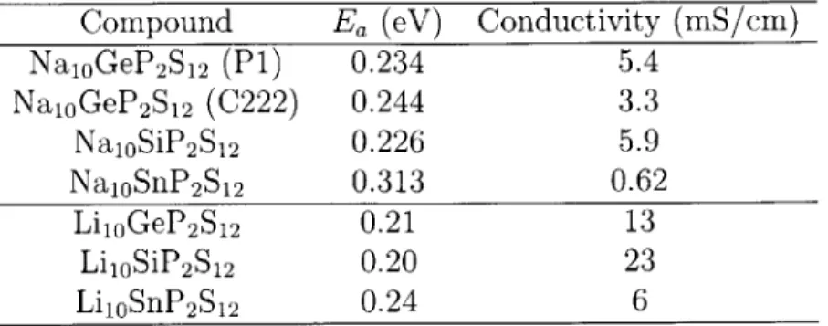
At low temperatures, even in superionic conductors, diffusion occurs on a long timescale relative to ab initio simulations. For materials with conductivity on the order of 10 mS/cm, each mobile atom experiences a single diffusive jump only every few hundred ps. Compared to the achievable timescales of ab initio MD (10s to hun-dreds of ps for small systems), simulation at room temperature is generally infeasible. For that reason, we perform simulation at elevated temperature, and extrapolate the conductivity at room temperature using an Arrhenius relation. This extrapolation assumes no change in the diffusive mechanism between the simulation temperature and desired operating temperature. For each structure, diffusivities were calculated at 8 temperatures between 600K and 1300K. For temperatures 1000-1300K, 200 ps were simulated. At the lower temperatures, simulations were extended to 400 ps to achieve better convergence. Arrhenius plots of the diffusivity are shown in figure 2-4. From these results, we calculate the diffusivity and extrapolated room temperature conductivity for the 4 structures (Table 2.3). For comparison, results from our study on the similar Li-ion electrolyte system are included[22].
Ea =234 meV * 0.8 1.0 1.2 1.4 1.6 1000FT (K- 1) (a) Ea =226 meV Se 0.8 1.0 1.2 1000FT (K- 1) (c) 1.4 1.6 -N E %L) -5.0 0 -5.5 45 E 0 -5.C 0 , E =244 meV a eS eS 0.8 1.0 1.2 1.4 1.6 1000FT (K- 1) (b) Ea =313 meV * '' '' S 0.8 1.0 1.2 1000/T (K-1)
Figure 2-4: Arrhenius plots for diffusivity
C222 symmetry (c) NaSiPS (d) NaSnPS
of: (a) NaGePS, P1 symmetry (b) NaGePS, -4.5 E 0-5. ,_-4.5 E %u -5.0 0 -- 5.1 1.4 1.6 (d)
In general, the diffusivities between the LMPS and NMPS systems are similar, which is expected given the similarity between the two frameworks. The activation energy for the Na materials are slightly higher than for their lithium counterparts. Similar to LMPS, NMPS is relatively unaffected by the choice of cation, though reveals the same trend of increasing E, across Si, Ge and Sn.
2.5
Conclusions
The NMPS system is in most respects very similar to LMPS. The intrinsic stabilities are comparable, with ground state structures 15 meV/atom above the hull. Like
LGPS, NGPS and its substitutions are found to be unstable against both the anode
and cathode with very similar decomposition products, though in most cases with less Na rich anode alloys of Si, Sn and Ge. Somewhat surprisingly, given the size difference of the mobile ion, even the activation energy for diffusivity is calculated to be only ~30 meV higher than LMPS for the Si and Ge versions. The extrapolated conductivities, ranging from 0.6 to 6 mS/cm for the various compositions, are high enough to rival existing liquid organic electrolytes. The relative order of diffusivity for the various cation substitutions of LMPS is also replicated in NMPS.
Chapter 3
Error bounds for diffusivity
calculations
While much of the previous discussion has been on a single class of materials, the search for a better solid electrolyte must extend beyond this narrow approach. In a broad search for new materials, it is important to be able to tune the tradeoff between precision of diffusivity measurements and the scope of material structures and chemistries. To do so efficiently requires an understanding of the error associated with the simulation and measurement of diffusivity. Typically, these errors are estimated
by making a large number of observations and invoking the central limit theorem so
that the mean value can be assumed to be normally distributed. A confidence interval is then constructed from the sample mean and variance.
With a limited computational budget, ideally one would run a simulation for the minimum amount of time such that a decision can be made on its suitability as a solid electrolyte, i.e. whether it passes some threshold in its conductivity. This chapter develops an understanding of the atomistic process of diffusion and the errors associated with measurements, so that these determinations can be made.
3.1
Diffusivity from the random walk
At the macroscopic scale, diffusivity is described by Fick's laws, which relate the flux of atoms to concentration or potential gradients via a simple linear relation:
J = -D-- 6(3.1) 6X
o#6
2q5= D 6(3.2)
6t 6x2
While useful for describing phenomena at macroscopic scales, this description does little to elucidate the diffusive mechanisms at work, and is infeasible to model via ab initio calculations due to the large system size required.
At an atomistic level, self diffusion arises from the random walk behavior of in-dividual atoms; the fluxes that Fickian diffusion models are due to small biases of otherwise random trajectories. The relationship between the random walk and the macroscopic diffusion constant is given by the Einstein-Smoluchowski diffusion rela-tion
((r - ro)2) = 2dDt (3.3)
where r is the atom displacement, d is the dimensionality of the system, D is the diffu-sivity, and t is the elapsed time. From an atomic simulation, diffusivity is determined
by measurement of the value of ((r - ro)2),
the mean squared displacement (MSD) of the diffusing species. While equation (3.3) holds in the long-time and many-particle limit, it breaks down at short timescales and for small numbers of atoms. The na-ture of diffusion sites in a crystal discretizes the allowable displacements and causes deviation from this idealized behavior.
On a discrete lattice, diffusivity can be expressed as a function of the lattice parameter and jump frequency:
D = (3.4)
2d
where F is the jump frequency, rj is the jump distance, d is the dimensionality of the system, and
f
is a correlation factor which is introduced to account for the fact thatjumps are not entirely random. In some cases, e.g. vacancy mediated diffusion, it is likely that after an atom has jumped to a neighboring vacancy, it will jump back to its original position due to the presence of the recently formed vacancy. In this case the correlation coefficient will have a value between 0 and 1. Similarly (though less frequently), there can be a tendency of a diffusing atom to continue in the direction of its most recent jump, and in this case the coefficient will be greater than 1. For the rest of this analysis, I define a new term rcorrelation , which is the average motion
caused by a single jump, as
rcorrelation = r f 1/2 (3.5)
With this simplification, correlated motion on a lattice with parameter r is very closely approximated by uncorrelated motion on a lattice with parameter rcorrelation.
Equations (3.4) and (3.3) are related by the expected MSD due to the random hopping at the limit of large times and large numbers of particles.
Fr 2orrelationt= ((r - ro)2) (3.6)
In the one dimensional case, the net motion of an atom during a simulation is given by the number of jumps it makes to the right (nr), minus the number it makes to the left (n1). The jump frequency F is modeled as the product of an attempt frequency
(related to the thermal vibration frequency) and a probability of overcoming an energy barrier Ea.
F = Ae-Ea/RT (3.7)
Probabilities of observing values of ni and n, are given by a binomial distribution, given the success probability and the attempt frequency
Pr(ni = k) = ) k(I _ P)tv-k, p = -Ea/RT (3.8)
I make one final assumption to further simplify the derivation of error bounds. I assume that the jump probability is small, which is justified by the fact that the
timescale for diffusion is typically much longer than for thermal vibration. This
sim-plifies the binomial distributions to Poisson distributions, and the net displacement of a single atom in one dimension to a Skellam distribution (the difference between two Poisson distributions).
/ dDt
r - To = TcorrelationSk(k; p1, P 2 = o )(3.9)
correlation
The Skellam distribution (Sk) typically takes two parameters, p, and P2, which are the expected number of events in each of the underlying Poisson distributions. For the case of diffusion, left and right diffusion are equally likely, so p1 = P2 = p. The
variance of this distribution is P1 + P2 = 2p. These p are a function of diffusivity,
so that the variance of position in equation (3.9) is compatible with the Einstein-Smoluchowski relation for large t.
3.2
Distribution of measurements of mean squared
displacements
This section discusses the distribution of observed values of the MSD given values for D and t. This distribution is directly derived from the underlying distribution of single atom displacement. This is done via a transformation of the distribution to account for the squaring of the displacement vector, and nob, convolutions of the distribution to take the mean.
fsquared(k; Pi, P2) = fskellam(k2; P1, P2) (3.10)
k k k
fmsd(k; pi, P2, nobs= fsquared( ) * fsquared( . * fsquared(
)
(3.11)ns nobs nobs
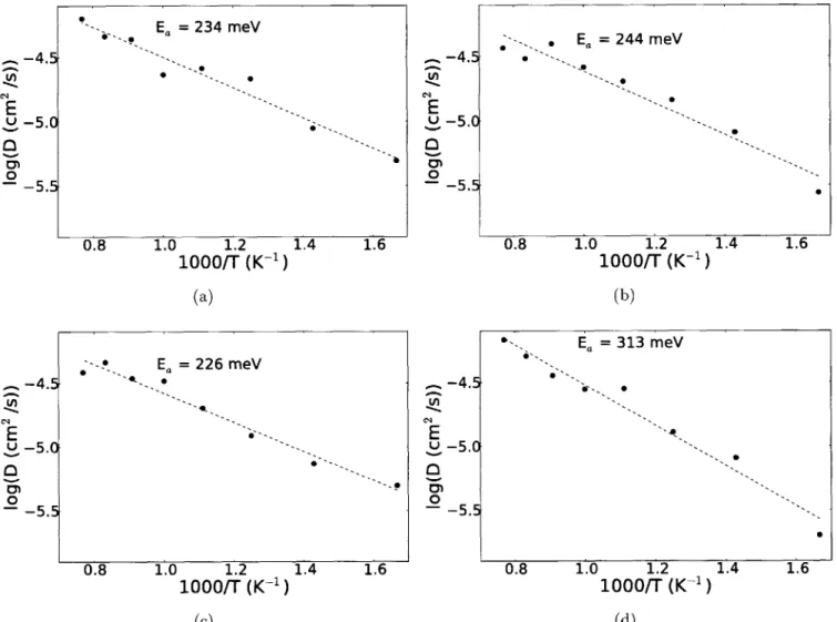
An example of the resulting distributions are given in figure 3-1. It can be seen that for small numbers of observations the convolution is extremely noisy, but smoothens as nobs increases. The discrete distributions are compared with the chi-squared tribution, which would result from starting with a normal, rather than skellam,
dis-020chi squared - chi squared
[ e keIIam 0.20 * squared skellam
0.15- 0.15-0.10 0.10-0.05- * 0.05-0.00 2 4 6 8 10 12 14 16 18 000 2 4 6 8 10 12 14 16 18 (a) (b)
Figure 3-1: Discrete MSD distributions with (a) nobs = 5,ip = 3 (b) nob, = 15,/p = 3
tribution.
Though it is possible to determine the likely values of D given this distribution, and the exact number of jumps taken by each atom, the non-smooth nature of the distribution often results in credible intervals that are not continuous. Additionally, in real simulations it can be difficult or impossible to completely remove the noise due to random thermal fluctuations of the structure.
3.2.1
Relating the theoretical distribution to simulation
ob-servables
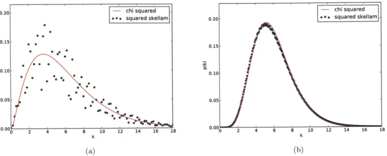
The Skellam distribution is a discrete distribution, though measurements in ab initio MD simulations are of a continuous quantity - atomic displacement. The discrepancy stems from the oscillations of atoms around their idealized lattice positions. These fluctuations are added to the model by the addition of a normally distributed contin-uous variable to the discrete atomic site motion. This is obtained by a convolution of the two distributions. Here I use a standard deviation of 0.2, which is typical for the ab initio MD results at relevant temperatures. Assuming this distribution, the
0.7 0.6- 0.10 -0.5 -0.08 - 0.4- 0.06- 0.3-0.04 0.2-0.02 0.1-0.0 - 0.020 0.0 -6 -4 -2 0 2 4 6 0.004 6 8 10 k k (a) (b)
Figure 3-2: (a) Single skellam variable + noise with p = 1 (b) MSD probability distribution with nobs = 3, p = 1
Figure 3-2 shows the individual atom displacement distribution as well as the MSD distribution with the addition of this noise. In these plots, the chi-squared distri-bution has been scaled to reflect the mean of the squared values, rather than the
sum.
It should be noted that the addition of the noise term causes the MSD distribution to converge to the chi-squared distribution for both small and large values of A. For small values of p, the noise term dominates. For large values of /p, the skellam distribution converges to a normal distribution plus some high frequency noise, which quickly disappears upon convolution. When p is close to 1, however, the effect of the excess kurtosis of the Skellam distribution cannot be ignored, and so the MSD distribution differs significantly from chi-squared.
3.3
A credible interval for MSD
So far, we have determined the distribution of MSD observations with a known value of Dt, though we need to determine Dt given some value of the MSD. In frequentist statistics, this is done by determining the confidence interval, but since the MSD
- skellam+noise
- normal
- squared skellam+noise
observations are significantly non-normal one cannot be constructed for the general case. Analogous to the idea of a confidence interval, in Bayesian statistics the credible interval defines a region in which the true underlying parameters of the distribution are likely to be found. Bayesian inference derives a probability distribution (the posterior probability) from some prior probability, and a likelihood function that is based on observed event.
P(HIE) =P(EH)P(H) (3.12)
P(E)
Our case of estimating a diffusivity parameter is relatively straightforward. E is the measured value of the MSD, P(HIE) is the probability distribution for the true value of Dt, P(H) is some prior distribution, and P(EIH) is the probability of observing our measurement for MSD, given some true value of the diffusivity (the likelihood function). The likelihood function is the previously derived distribution of
MSD measurements.
Given any observed MSD data, the posterior probability of the underlying values of Dt can be calculated. The credible interval is then constructed as the region between 0.1 and 0.9 on the CDF of this distribution.
3.3.1
Choosing a prior distribution
The last decision required is that of the prior probability distribution. While it is possible to construct a prior distribution from the diffusivities of known compounds, it is often desirable to use an uninformed prior, which adds as little information about the distribution as possible. For the case of diffusion, where we estimating a parameter on the interval [0, inf), two such uninformed priors are relevant - the uniform distribution and the log-uniform distribution. We will see that both of these priors have their own complications, and to be conservative a combination of the two must be used.
Log-Uniform distribution
The log uniform distribution seems at first glance to be a perfect choice for a prior. It is invariant to a number of reparameterisations, and diffusivity values span many orders of magnitude. This prior distribution gives the same weight to the interval (1,
10) as it does to (le-4, le-3), which is desirable. An issue arises, however, because
the observed values are due to a diffusive term plus a constant noise term. For low observed MSD, it is possible that the observation is entirely due to noise, and so the PDF of D becomes constant below some value. With this prior, the lower bound of the credible interval is 0, as it should be, but the upper bound is also infinitely small.
Uniform distribution
The use of a uniform prior distribution eliminates the issue of undefined bounds on the credible interval, but does so at the expense of overweighting high diffusivities. Our intuitive notion that diffusivities are log-normally or log-uniformly distributed is somewhat valid (the distinction between these isn't of particular importance when using a log-uniform prior) but the assumption of a uniform prior weights the interval
(0.1,1) with le6 times the weight of (le-7, le-6). This leads to cases where the lower
bound on the credible interval exceeds the observed MSD value (even though the observed MSD has been increased by the addition of noise).
Reconciliation of these distributions
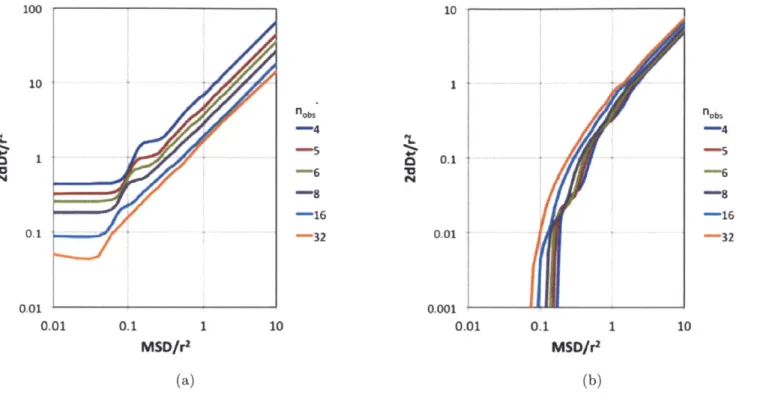
The use of the log-uniform prior for determining a lower bound on diffusivity mea-surements and the uniform prior for determining the upper bounds yields an interval that is numerically stable, and somewhat conservative. For comparison, the 90% up-per bound of an observation of MSD = 30 with nobs = 4 is 112 with the log-normal prior, but 200 with the uniform prior. As nobs increases, the difference in priors is less significant; for nobs = 16, the upper bounds are 51 and 60 respectively.
The credible intervals built from these prior distributions for observed values of MSD and given rcorrelaton are given in figure 3-3. It should be noted that the width
100 10
z
nob nobs m44 -s 0.1 16 16 0.1 -32 0.01 -32 0.01 0.001 0.01 0.1 1 10 0.01 0.1 1 10 MSDOr 2 MSD/r 2 (a) (b)Figure 3-3: Bounds as a function of MSD for various nobs: (a) upper bound with uniform prior (b) lower bound with log-uniform prior
of the credible interval depends both on the number of observations and the amount of diffusion observed. The number of observations is the number of mobile atoms observed over independent time intervals, i.e. if a simulation including 5 Li atoms is run for 200 ps, this can be used as 5 200 ps observations, or split into 10 100ps observations.
3.4
Comparison of Bayesian credible intervals to
the Frequentist confidence interval
The Bayesian method of determining a credible interval is attractive in that it can be used for any observed values of MSD. The general non-normality of the data makes a confidence interval impossible to obtain, except in special circumstances. When the number of MSD observations is large, the central limit theorem holds and the mean MSD value can be assumed to be normally distributed. More usefully, since
individual atomic motion is at long times normally distributed, all that needs to be calculated is a confidence interval on the variance of this distribution. Since the mean is known (0), this is given by
___ 2_ < o. 2 < 2_(3.13)
x2(1 - a/2; k) x2(a/2; k)
It the other extreme, where no diffusive jumps are observed, the distribution approaches the Poisson distribution. For a poisson distribution with parameter A, the confidence interval for confidence level a of the poisson distribution is
12 12
2x(a/2; 2k) A x (1 - a/2; 2k + 2) (3.14)
For a 90% upper bound, this is equal to 2.3/k. This corresponds approximately to the low MSD limit of the Bayesian confidence interval with a uniform prior for low numbers of observations. As the number of observations increases and the sum of squared noise terms approaches one, the distributions diverge. For typical ab initio MD simulations, the number of diffusing atoms is on the order of 10 or 20, so this divergence isn't an issue. For larger simulations, better error bounds could be obtained by attenuating this noise.
These limiting cases (figure 3-4) show the compatibility of the two methods. The advantage of the Bayesian approach is that it can be used with small MSD obser-vations, while if any diffusion is observed a much longer (approx. 10x) simulation must be run before one can be confident in the validity of applying the central limit theorem.
3.5
Summary
This chapter developed a method for generating confidence intervals on data which is known to be strongly non-normal. At its extremes, the upper bound approaches bounds of well-studied distributions; for low MSD and low numbers of atoms it ap-proaches the upper bound on a Poisson parameter, and for large MSD it apap-proaches
100 10 Bayesian Poisson Chi-squared 0.1 0.01 0.001 0.01 0.1 1 10 MSD/r 2
Figure 3-4: Comparison of Bayesian upper bound with bounds based on Poisson and Chi squared distributions for nm = 6
the chi-squared distribution. The confidence intervals produced are applicable to any
MSD observation, a wide range of which are not well described by either a Poisson
process or by normally distributed data. The deviation from the Poisson confidence interval for low-MSD high-nob, is due to atomic vibrations, and with additional data processing can be reduced. For typical ab initio MD simulations, however, this is not necessary.
Bibliography
[1]
S. Adams and R. P. Rao. High power lithium ion battery materials bycompu-tational design. Phys. Status Solidi, 208(8):1746-1753, Aug. 2011.
[2] S. Adams and R. P. Rao. Ion transport and phase transition in Li7-_La3(Zr 2-xMx)O 2 (M = Ta5+, Nb5+, x = 0, 0.25). J. Mater. Chem., 22(4):1426, 2012.
[3] P. Balakrishnan, R. Ramesh, and T. Prem Kumar. Safety mechanisms in
lithium-ion batteries. J. Power Sources, 155(2):401-414, Apr. 2006.
[4] P. B16chl. Projector augmented-wave method. Phys. Rev. B, 50(24), 1994.
[5] A. Chroneos, D. Parfitt, J. a. Kilner, and R. W. Grimes. Anisotropic oxygen
diffusion in tetragonal La2NiO4+6: molecular dynamics calculations. J. Mater.
Chem., 20(2):266, 2010.
[6] C. Dellago and P. Bolhuis. Transition path sampling and other advanced
simu-lation techniques for rare events. Adv. Comput. Simul. approaches ... , 2009.
[7] M. Ernzerhof and G. E. Scuseria. Perspective on "Inhomogeneous electron gas".
Theor. Chem. Accounts Theory, Comput. Model. (Theoretica Chim. Acta),
103(3-4):259-262, Feb. 2000.
[8] H. Grubmiiller. Predicting slow structural transitions in macromolecular
sys-tems: confomational flooding. Phys. Rev. E, 1995.
[9] G. Henkelman, B. P. Uberuaga, and H. Jonsson. A climbing image nudged elastic
band method for finding saddle points and minimum energy paths. J. Chem.
Phys., 113(22):9901, 2000.
[10] N. Holzwarth, N. Lepley, and Y. a. Du. Computer modeling of lithium phosphate
and thiophosphate electrolyte materials. J. Power Sources, 196(16):6870-6876, Aug. 2011.
[11] A. Jain, G. Hautier, C. J. Moore, S. Ping Ong, C. C. Fischer, T. Mueller, K. a.
Persson, and G. Ceder. A high-throughput infrastructure for density functional theory calculations. Comput. Mater. Sci., 50(8):2295-2310, June 2011.
[12] H. Jonsson, G. Mills, and K. Jacobsen. Nudged elastic band method for finding minimum energy paths of transitions. In Class. quantum Dyn. Condens. phase
simulations, pages 385-404. 1998.
[13] N. Kamaya, K. Homma, Y. Yamakawa, M. Hirayama, R. Kanno, M. Yonemura,
T. Kamiyama, Y. Kato, S. Hama, K. Kawamoto, and A. Mitsui. A lithium superionic conductor. Nat. Mater., 10(9):682-686, July 2011.
[14] M. S. Khan. Cation doping and oxygen diffusion in zirconia: a combined atom-istic simulation and molecular dynamics study. J. Mater. Chem.,
8(10):2299-2307, 1998.
[15] M. Kilo and C. Argirusis. Oxygen diffusion in yttria stabilised
zirconiaexperimen-tal results and molecular dynamics calculations. Phys. Chem. ... , 5(11):2219,
2003.
[16] S.-W. Kim, D.-H. Seo, X. Ma, G. Ceder, and K. Kang. Electrode Materials for
Rechargeable Sodium-Ion Batteries: Potential Alternatives to Current Lithium-Ion Batteries. Adv. Energy Mater., 2(7):710-721, July 2012.
[17] G. Kresse and J. Furthmiiller. Efficient iterative schemes for ab initio
total-energy calculations using a plane-wave basis set. Phys. Rev. B. Condens. Matter,
54(16):11169-11186, Oct. 1996.
[18] A. Kuhn, J. Koehler, and B. V. Lotsch. Single-Crystal X-ray Structure
Anal-ysis of the Superionic Conductor Lii0GeP2S12. Phys. Chem. Chem. Phys.,
15(28):11620-2, July 2013.
[19] Z. Liu, W. Fu, E. A. Payzant, X. Yu, Z. Wu, N. J. Dudney, J. Kiggans, K. Hong, A. J. Rondinone, and C. Liang. Anomalous high ionic conductivity of nanoporous
/3-LiPS4. J. Am. Chem. Soc., 135(3):975-8, Jan. 2013.
[20] R. Marom, S. F. Amalraj, N. Leifer, D. Jacob, and D. Aurbach. A review of advanced and practical lithium battery materials. J. Mater. Chem., 21(27):9938, 2011.
[21] Y. Mo, S. Ong, and G. Ceder. First principles study of the Lij0GeP 2S12 lithium
super ionic conductor material. Chem. Mater., pages 12-14, 2011.
[22] S. Ong, Y. Mo, W. Richards, and L. Miara. Phase stability, electrochemical stability and ionic conductivity of the LiioiiMP2X1 2 (M= Ge, Si, Sn, Al or P,
and X= 0, S or Se) family of superionic conductors. Energy Environ. Sci., 6(1):148, 2013.
[23] S. P. Ong, W. D. Richards, A. Jain, G. Hautier, M. Kocher, S. Cholia, D. Gunter,
V. L. Chevrier, K. a. Persson, and G. Ceder. Python Materials Genomics (py-matgen): A robust, open-source python library for materials analysis. Comput.
[24] S. P. Ong, L. Wang, B. Kang, and G. Ceder. Li-Fe-P-0 2 Phase Diagram from First Principles Calculations. Chem. Mater., 77(4):755-759, 2008.
[25] V. Palomares, M. Casas-Cabanas, E. Castillo-Martinez, M. H. Han, and T. Rojo.
Update on Na-based battery materials. A growing research path. Energy Environ.
Sci., 6(8):2312, 2013.
[26] J. Perdew, K. Burke, and M. Ernzerhof. Generalized Gradient Approximation
Made Simple. Phys. Rev. Lett., 77(18):3865-3868, Oct. 1996.
[27] J. Sanchez, J. Fullea, M. Andrade, and P. D. Andres. Ab initio molecular
dy-namics simulation of hydrogen diffusion in ac-iron. Phys. Rev. B, pages 1-14, 2010.
[28] J. Sarnthein, K. Schwarz, and P. Bl6chl. Ab initio molecular-dynamics study of
diffusion and defects in solid Li3N. Phys. Rev. B, 53(14):9084-9091, Apr. 1996.
[29] A. Voter. Hyperdynamics: Accelerated molecular dynamics of infrequent events.
Phys. Rev. Lett., 1997.
[30] L. Wang, T. Maxisch, and G. Ceder. A First-Principles Approach to Studying
the Thermal Stability of Oxide Cathode Materials. Chem. Mater., 19(3):543-552, Feb. 2007.
![Figure 2-1: Structures of LGPS determined from (a) Kamaya et al.[13] and (b) Kuhn et al.[18]](https://thumb-eu.123doks.com/thumbv2/123doknet/13812623.441916/20.918.166.758.155.473/figure-structures-lgps-determined-kamaya-et-al-kuhn.webp)