HAL Id: hal-01149529
https://hal.inria.fr/hal-01149529v3
Submitted on 8 Jun 2015
HAL is a multi-disciplinary open access
archive for the deposit and dissemination of
sci-entific research documents, whether they are
pub-lished or not. The documents may come from
teaching and research institutions in France or
abroad, or from public or private research centers.
L’archive ouverte pluridisciplinaire HAL, est
destinée au dépôt et à la diffusion de documents
scientifiques de niveau recherche, publiés ou non,
émanant des établissements d’enseignement et de
recherche français ou étrangers, des laboratoires
publics ou privés.
LMI-based 2D-3D Registration: from Uncalibrated
Images to Euclidean Scene
Danda Pani Paudel, Adlane Habed, Cedric Demonceaux, Pascal Vasseur
To cite this version:
Danda Pani Paudel, Adlane Habed, Cedric Demonceaux, Pascal Vasseur. LMI-based 2D-3D
Registra-tion: from Uncalibrated Images to Euclidean Scene. CVPR 2015 - 28th IEEE Conference on Computer
Vision and Pattern Recognition, Jun 2015, Boston, United States, Jun 2015, Boston, United States.
�hal-01149529v3�
LMI-based 2D-3D Registration: from Uncalibrated Images to Euclidean Scene
Danda Pani Paudel
1, Adlane Habed
2, C´edric Demonceaux
1, Pascal Vasseur
31
Le2i laboratory, University of Bourgogne, CNRS, France
2ICube laboratory, University of Strasbourg, CNRS, France
3
LITIS EA laboratory, University of Rouen, France,
{danda-pani.paudel,cedric.demonceaux}@u-bourgogne.fr
,
[email protected],
Abstract
This paper investigates the problem of registering a scanned scene, represented by 3D Euclidean point coordi-nates, and two or more uncalibrated cameras. An unknown subset of the scanned points have their image projections detected and matched across images. The proposed ap-proach assumes the cameras only known in some arbitrary projective frame and no calibration or autocalibration is required. The devised solution is based on a Linear Matrix Inequality (LMI) framework that allows simultaneously es-timating the projective transformation relating the cameras to the scene and establishing 2D-3D correspondences with-out triangulating image points. The proposed LMI frame-work allows both deriving triangulation-free LMI cheirality conditions and establishing putative correspondences be-tween 3D volumes (boxes) and 2D pixel coordinates. Two registration algorithms, one exploiting the scene’s structure and the other concerned with robustness, are presented. Both algorithms employ the Branch-and-Prune paradigm and guarantee convergence to a global solution under mild initial bound conditions. The results of our experiments are presented and compared against other approaches.
1. Introduction
With the ongoing surge in affordable high quality 3D and 2D capture sensors, the two modalities are increasingly of-ten jointly used in vision-based systems. Using informa-tion from both 2D and 3D sensors, such as a laser scan-ner or RGB-D camera, provides several advantages rang-ing from texture mapprang-ing to scene understandrang-ing. It, how-ever, may also come with its share of difficulties and chal-lenges. When the 3D sensor and 2D cameras are rigidly attached, the system can be calibrated at once. If the two
sensor modalities are free, many such systems require the 2D cameras to be internally calibrated and registered with the 3D sensor at all time. Camera calibration can be carried out either by using a dedicated pattern in the scene or via autocalibration. The registration of the 2D cameras and the 3D sensor is generally achieved by establishing correspon-dences in two ways: (i) between scanned 3D data and 2D features; (ii) between scanned 3D points and 3D triangu-lated points from calibrated cameras.
The problem of establishing correspondences between 3D data and 2D features has been tackled in [23] for points, [5] for lines, [12] using planes, [22] using skylines and [13] by relying on scene constraints. The success of such methods is often undermined by the absence of re-liable 3D descriptors and their lack of compatibility with 2D descriptors. They may also be undermined by the like-wise unreliable descriptors for certain image features such as lines. Other registration methods are based on mutual information [29] and region segmentation [27] but suffer from similar drawbacks. Establishing correspondences be-tween scanned and triangulated 3D points is often carried out using the Iterative Closest Point (ICP) algorithm. The image-induced scene may however be reconstructed only up to a scale ambiguity making the problem particularly diffi-cult to solve. In [6], this ambiguity is handled by an ex-tension of the 4-points congruent sets algorithm [1]. Other scale-invariant registration methods perform registration ei-ther by a voting approach [19] or performing mean-shift in the scale invariant space [20]. None of these methods guar-antees convergence to a globally optimal solution. The re-cent Go-ICP method, proposed in [30], is a globally opti-mal method for registering 3D point clouds with the same scale. The scale of the image-induced 3D scene can only be corrected with additional knowledge. However, using any of [6,19,20,30] requires the cameras to be calibrated.
This paper investigates the problem of registering a scanned scene, represented by Euclidean 3D point coor-dinates, and two or more uncalibrated cameras. An un-known subset of the scanned points have their image pro-jections detected and matched across images. The pro-posed approach assumes camera matrices to be calculated in some arbitrarily chosen projective frame and no cali-bration or autocalicali-bration is required. We argue here that camera calibration may turn out to be impractical due to possible changes in the cameras’ internal geometry when zooming and focusing. As for camera autocalibration, al-though globally convergent methods [8, 3,4,9] do exist, the process fails for numerous critical motions of the cam-eras and is generally sensitive to 2D pixel localization er-rors. When cameras are uncalibrated, the transformation relating the cameras to the scene is projective. Our pro-posed registration solution is based on a Linear Matrix In-equality (LMI) framework that allows simultaneously esti-mating this unknown projective transformation and estab-lishing 2D-3D correspondences without triangulating im-age points. The proposed LMI framework allows both de-riving triangulation-free LMI cheirality conditions and es-tablishing putative correspondences between 3D volumes (boxes) and 2D pixel coordinates. Directly using raw 2D points in lieu of triangulated 3D points is believed to yield more accurate motion computation [24]. In practice, trian-gulation results are rather uncertain in the depth direction. Using a small set of such reconstructed points for alignment may have a devastating effect on the results [17].
Two registration algorithms, one exploiting the scene’s structure and the other concerned with robustness, are pre-sented. Both algorithms employ the Branch-and-Prune paradigm and guarantee convergence to a global solution under some mild initial bounding conditions. Our algo-rithms require initial box-2D correspondences with 5 non-overlapping boxes to guarantee convergence to a global so-lution. Alternatively, non-overlapping bounds on camera centers can also be used. Finding initial bounds on cam-era positions is relatively easy as far as hand-held or GPS-equipped cameras are concerned. The results of our experi-ments, on both simulated and real data, are also presented.
2. Background and notations
Consider a static scene consisting of m 3D points {Xj}mj=1observed byn ≥ 2 uncalibrated 2D pinhole
cam-eras{Pi}n
i=1. Scene points and cameras may be retrieved
from point correspondences across images up to an un-known projective ambiguity. Let Pi be the 3 × 4 matrix representation ofPi and X
j the homogeneous coordinate
vector ofXj, all expressed in a common projective frame.
The special pointCi, with coordinates Ciin this frame
sat-isfying PiC
i= 0 (0 is the null-vector), is the optical center
of cameraPi. The 2D pixel projectionxi
j of a scene point
Xjonto cameraPi is given by xij ∼ PiXj where∼ refers
to the equality up to an unknown scale.
Triangulation: Any pointXj can be triangulated in a 3D
coordinate frame given camera matrices and 2D pixel cor-respondences{xi
j}ni=1 across images. So long as at least
two 2D points are matched in at least two images, if a xi j
is unknown in one given image (no corresponding feature point detected and/or matched in that image), it can safely be replaced by the null vector without prejudice for what follows. Let Sjbe the3n × 3n block-diagonal matrix
Sj = diag([ x1j]×, [ x2j]×, [ x3j]×, . . . [ xnj ]×) (1)
with matrices[ xi
j]×,i = 1 . . . n, on the diagonal blocks and
zeros elsewhere.[ xi
j]×denotes the3 × 3 skew-symmetric
matrix associated with the cross-product and constructed using the projection xijofXjon cameraPi. Let M be the
3n × 4 matrix obtained by stacking all camera matrices: M!= [ P1!P2!P3!. . . Pn!].
(2) The coordinate vector ofXjcan then be obtained by solving
SjMXj = 0. Note that matrix SjM must be of rank-3, or
else assumed to be enforced as such throughout this paper. Cheirality: As far as the true Euclidean camera matrices and 3D points are concerned, the depth of any scene point, relative to a camera in which it is visible, must be posi-tive. The sign of this depth is referred to as the cheirality of the point with respect to the considered camera [11,10]. However, in addition to the projective ambiguity, projective points and cameras are each retrieved up to a different un-known scale generally not preserving cheirality. It is possi-ble though to assign signaturesζi= ±1 to cameras and
sig-naturesηj = ±1 to points to ensure that: (i) each point has
a consistent cheirality with respect to all cameras in which it is visible, and (ii) all points have a consistent cheirality with respect to any one camera in which they are visible. Camera signatures: LetX be a point visible in camera P . The cheirality ofX with respect to any camera Piin which
it is also visible must be identical to that of its cheirality with respect toP . This can be enforced by considering the signaturesζ and ζiof, respectively,P and Pisuch that
(ζPX)3(ζiPiX)3> 0forXvisible inPandPi. (3)
Note that (3) can be used to deduce the signature of one camera given the signature of the other. Indeed, this can be done by initially assigning an arbitrarily chosen signatureζ to one given cameraP and iteratively assigning signatures to all cameras observingX. Every Pi with assigned
sig-nature can in turn be used to deduce sigsig-natures of cameras sharing visible points with it. A robust version of such al-gorithm may be found in [16].
Point signatures: Correcting the signatures of cameras suf-fices to enforce identical cheirality for any given point in all
the views in which it is visible. It, however, remains that any two pointsX and Xj, visible in the same cameraP , may
have different cheiralities,(PX)3(PXj)3 < 0, with respect
to that camera. To make such points share the same cheiral-ity relative to one such camera, one seeks the signaturesη andηjof these points such that
(ηPX)3(ηjPXj)3> 0forXandXjvisible inP. (4)
Using (4), one may arbitrarily assign a signatureη to one of the pointsX and recover the signatures of the remaining visible points. Once a signature is assigned to a point, it can be used to assign signatures to points visible in other views. Cheirality inequalities: Note that(3) allows to assign sig-natures to cameras independently from the homogeneous representation of the considered visible points. Likewise, signatures are assigned to points through (4) independently from the camera signatures. However, this suffices to guar-antee that the cheirality of any point to be identical with respect to all cameras in which it is visible. It also guar-antees that all points visible by one camera carry the same cheirality with respect to it. As in the Euclidean frame, once signatures are assigned to cameras and points, the plane at infinityΠ∞neither cuts through the convex hull of scene
points nor does it cut through the convex hull of camera centers. The projective coordinates ofΠ∞must satisfy:
ηjΠ!∞Xj>0 for j = 1 . . . m, (5)
δζiΠ!∞Ci>0 for i = 1 . . . n (6)
for someδ = ±1. Note that the coordinate vectors Ci
re-ferred to in (6) ought to be obtained exactly through the identity C!
iΠ= det([P
i!| Π]) for some 4-vector Π.
Upgrade: The plane at infinity plays a key role in upgrad-ing a projective reconstruction to its Euclidean or affine counterpart. For instance, the Euclidean coordinates XEj of pointsXj and Euclidean camera matrices P
Ei
ofPi,
satis-fying xij ∼ PEi
XE
j, are only a projective transformation, say
H, away from their projective counterparts: XE
j ∼ HXjand
PEi ∼ PiH−1. The full-rank4 × 4 matrix H is the matrix
representation ofH. Unless the cameras are calibrated and their pose calculated, H is unknown. However, the last row of H is the homogeneous coordinate vector Π∞of the plane
at infinity in the projective frame. If the latter is known, for arbitrarily chosen remaining rows of H, points at infinity in the true scene are mapped back onto the canonical plane. In this case, the scene and cameras are said to be reconstructed in an affine frame. Π∞being generally unknown, one may
use a surrogate plane, say !Π∞whose coordinate vector ˜Π∞
in the projective frame satisfies (5) and (6). The resulting reconstruction is then said to be quasi-affine with respect to the considered points and camera centers.
LMIs and SDPs: When dealing with matrices, A > 0 (resp. A ≥ 0 ) means that the symmetric matrix A is positive-definite (resp. positive semi-definite). A Linear
Matrix Inequality (LMI) is a constraint on a real-valued vec-tor y = (y1, y2, . . .) such that A(y) > 0. The matrix
A(y) = A0+"iyiAi is an affine function of y
involv-ing symmetric matrices A0, A1, A2. . .. A LMI feasibility
problem consists in finding y that satisfies the considered LMI or determining that no solution exists. It is a convex optimization problem that can be efficiently solved using interior-point methods [2]. When a LMI A(y) > 0 arises in homogeneous form, i.e. A(y) ="iyiAi, it is replaced
by a non-homogeneous counetrpart A(y) ≥ I as to avoid numerical issues since A(0) = 0. A Semidefinite program (SDP) consists in minimizing or maximizing a linear ob-jective subject to LMI constraints. A key ingredient in the work presented in this paper is the following lemma: Lemma 2.1 (Finsler’s) Let Y be a vector, Q a symmetric matrix, B a rectangular matrix - all real-valued and of ap-propriate dimensions - andγ a scalar. The following state-ments are equivalent:
(i) Y!QY >0 ∀Y ̸= 0: BY = 0.
(ii) ∃ γ: Q + γB!B >0.
Lemma2.1is due to Paul Finsler [7]. It allows to convert the problem of checking the sign of a quadratic form over a subspace into solving a LMI problem.
Further notations: Additional notations are used through-out the paper: the canonical vectors are denoted ek, k =
1, 2, 3, such that e1 = (1 0 0)!, e2 = (0 1 0)! and
e3 = (0 0 1)!. The superscript ⋆ refers to the
symmet-ric part of a square matrix. For example, the symmetsymmet-ric part Q⋆of a square matrix Q is given by Q⋆= 1
2(Q + Q
!).
3. LMI-based 2D-to-3D registration
In this section, we first introduce a set of LMI and bounding conditions that constitute the backbone of our 2D-3D registration algorithms. The proposed algorithms are also presented in this section. We consider the scene im-aged by a sequence of uncalibrated cameras and scanned by a 3D sensor. In addition to 2D point correspondences across images, the scanned scene points are given by their Euclidean coordinates XE
j, j = 1 . . . m. In the absence
of Euclidean-to-projective (3D-3D) point correspondences and Euclidean-to-image (3D-2D) point correspondences, the scanned points are an unknown projective transforma-tion away, XEj ∼ HXj, from the image-induced 3D points
Xj. Note that H can be linearly calculated if 3D-3D point
correspondences are available. It can also be estimated from 3D-2D point correspondences via xij ∼ PiH−1X
E
j. It goes
without saying that, if H is known, then the correspondences can be established. However, when neither H nor 3D-3D or 3D-2D correspondences are known, the problem is particu-larly challenging and difficult to solve. Our goal is precisely to simultaneously establish such unknown correspondences
and estimate H while using only 2D pixel coordinates and the Euclidean coordinates of the scanned points: i.e. with-out triangulating image points in 3-space. Once the corre-spondences established and H estimated, the Euclidean ma-trices PEi
, camera pose and internal calibration parameters can be extracted. Our proposed solution heavily depends upon finding a surrogate plane at infinity !Π∞that wouldn’t
cross the scene and cameras. This however traditionally re-quires the so-called cheirality inequalities involving image points to be triangulated. Therefore, prior to presenting our registration conditions and methods, we first provide a LMI formulation of the cheirality inequalities for obtaining such “quasi-affine” plane without triangulating image points.
3.1. Cheirality LMIs
Consider a point X visible in camera P . The signa-tureζ of P and that of any camera Pi in whichX is also
visible must satisfy (3). Note that (3) can be rewritten as ζζiX!P!e3e!3PiX > 0. One can only notice that the
lat-ter inequality is equivalent to ζζiX!(P!e3e!3Pi)⋆X > 0
when employing the symmetric part of the involved matrix. Finsler’s lemma can then be used to deduce the LMI
∃γ : ζζi(P!e3e!3Pi)⋆+ γi(SM)!SM> 0 (7)
for X visible inP and Pi. In (7),γiis a scalar and matrices
S and M are constructed as in (1) and (2) from the image projections of pointX and camera matrices. Note that LMI (7) is equivalent to (3). It allows to correct the signature of a camera given the signature of another camera. Unlike (3), LMI (7) does not require triangulating any pointX. As in (3), an arbitrary signatureζ can initially be assigned to camera P and every matrix whose signature is recovered can be used to deduce the signatures of other cameras.
An alternative to (4) would be to enforce that all points Xjvisible in some cameraPi have positive cheirality, i.e.
ζiηje!3PiXj > 0 as demanded when using the true
Eu-clidean points and cameras. From (5), one can deduce thatηj and X!jΠ∞must carry the same sign. Because Π∞
is homogeneous, we can choose the plane at infinity such that ζiX!jΠ∞e
!
3PiXj > 0. The latter inequality remains
true when considering the symmetric part of the matrix in-volved: X!
j(ζiΠ∞e!3Pi)⋆Xj > 0. Using Finsler’s lemma
and accounting for homogeneity, we deduce that LMI (ζiΠ∞e!3Pi)⋆+ γji(SjM)!SjM> I (8)
must hold for any point Xj visible inPi for some scalar
γi
j and the true Π∞. Given the signatures of all cameras
obtained via (7), LMI (8) is an equivalent alternative to us-ing (5) to calculate a “quasi-affine” plane !Π∞, satisfying
(8), not cutting through the convex-hull of visible points. Unlike (5), LMI (8) neither requires the calculation of point signatures nor does it require the reconstruction of the ob-served points in 3-space. A surrogate plane at infinity !Π∞
can be obtained by solving the LMIs (8) along with inequal-ities (6) (withδ = ±1) for all cameras and visible points.
3.2. Bounding LMIs
Definition 3.1 (Positive vs. negative sides of a plane) Consider a plane Π with Euclidean coordinate vector ΠE
. We say that a point X with coordinates XE
in this frame lies on the positive side with respect to this plane if and only if XE!ΠE
∞ΠE!X
E
> 0. The coordinate vector ΠE
∞ = (0 0 0 1)! is that of the plane at infinity in the
Euclidean frame. Points on the negative side with respect Π satisfy XE!ΠE
∞ΠE!X
E
< 0.
Definition 3.2 (Boxing a point) Let B = {(Πk, Πk)}3k=1
be a set of three pairs of planes with Euclidean coordinate vectors ΠEk = (e! k − dk)!and Π E k = (e ! k − dk)!such that
the signed distancesdk anddk of the planes to the origin
of the frame satisfy dk < dk. Without loss of generality,
the normal vectors ek of the planes are assumed to be the
canonical basis vectors. We say that a pointX is boxed by B if for each pair (Πk, Πk), X is on the positive side with
respect toΠkand negative side with respect toΠk.
Let Sj be the matrix constructed as in (1) from 2D
matches. Let ME
(resp. M) be, as in (2), the stack of Eu-clidean (resp. projective) camera matrices PEi
(resp. Pi) ,
i = 1 . . . m. Based on the above definitions, the following corollary can be directly deduced from Finsler’s lemma. Corollary 3.3 A point Xj projecting ontoxij in cameras
{Pi}n
i=1 is boxed byBj = {(Πk, Πk)}3k=1 if and only if
the following LMIs are simultaneously feasible for some scalarsγ jkandγjk: (ΠE∞Π E! k ) ⋆ + γ jk(SjM E )!S jM E >0 k = 1, 2, 3 (9) γjk(SjM E )!S jM E − (ΠE ∞Π E! k ) ⋆ >0 k = 1, 2, 3. (10)
Remark 3.4 Note that if any of LMIs (9) and (10) is fea-sible for someγjk, then the same LMI is also feasible for
anyγ > γjk. Hence, one can seek a singleγ
simultane-ously satisfying (9) and (10) rather than six scalarsγ
jk,
γjk(k = 1, 2, 3) for each point. This also means that a sin-gleγ can be sought for the LMIs induced by multiple points Xj. We henceforth express all our LMIs using a commonγ.
Corollary3.3allows to express the correspondence be-tween a box in 3D and 2D point matches. It basically states that if the 3D pointXj was to be triangulated from 2D
cor-respondences{xi
j}mi=1, then it would be within the boxBj
if LMIs (9) and (10) were feasible and outside this box oth-erwise. However, LMIs (9) and (10) depend upon the un-known Euclidean camera matrices and the true plane at in-finity. Let us now consider the block-diagonal matrix
Bj= diag(B1j, B 2 j, B 3 j, B 1 j, B 2 j, B 3 j) (11)
whose blocks Bkj = (!Π∞ΠE!k H)⋆+γ(SjM)!SjM and B k
j =
γ(SjM)!SjM−(!Π∞Π E!
k H)⋆are expressed using projective
camera matrices, an unknown4 × 4 transformation matrix H, and the surrogate plane at infinity !Π∞(calculated as in
Section3.1). The following holds for visible scene points: Proposition 3.5 LetSx = {(Xj, Bj)}mj=1be a set of
puta-tive point-to-box correspondences (i.e. each pointXj,
pro-jecting onto image points{xi
j}ni=1, is assigned to a boxBj).
IfSx’s correspondences are correct then LMIs
Bj≥ I, j = 1 . . . m (12)
must be simultaneously feasible for a scalarγ and at least the true transformation matrix H satisfying XE
j ∼ HXj.
Proof The proof relies on Corollary3.3. Recall that ME∼ MH−1 and Π
∞ = H!ΠE∞. It is well-known that
congru-ence transformations preserve definiteness. Hcongru-ence, pre- and post-multiplying the left-hand side of each of LMIs (9) and (10) by H and H!, these can be respectively rewritten as
(Π∞ΠE!k H)⋆ + γ(SjM)!SjM > 0 and γ(SjM)!SjM−
(Π∞Π E!
k H)⋆> 0. As per Remark3.4, a commonγ is used.
Because X!
jΠ∞Π!!∞Xjcarry the same sign for all pointsXj,
one can replace Π∞by !Π∞thus leading to all Bkj and B k j
being simultaneously either positive or negative definite. Since H is unknown, one may choose to enforce positive rather than negative definiteness. Bj > 0 then arises
nat-urally since a block-diagonal matrix is positive-definite if and only if each of its diagonal blocks is positive-definite. Because Bj > 0 is homogeneous, it is replaced by (12).
Similarly, consider the matrix Di= diag(D1i, D 2 i, D 3 i, D 1 i, D 2 i, D 3 i) (13)
with blocks Dki = δ(!Π∞ΠE!k H)⋆ + γPi!Pi and D k
i =
γPi!Pi− δ(!Π
∞Π
E!
k H)⋆. Given !Π∞andδ, both obtained
by solving (6) and cheirality LMIs (8), the following holds:
Proposition 3.6 LetSc = {(Ci, Ci)}ni=1be a set of
puta-tive camera-to-box correspondences (i.e. each camera cen-terCiis assigned to a boxCi). IfSc’s correspondences are
correct, then LMIs
Di≥ I, i = 1 . . . n (14)
must be simultaneously feasible for a scalarγ and at least the true transformation matrix H satisfying XEj ∼ HXj.
Proof The proof, omitted here, is along the lines of that of Proposition3.5. It employs Finsler’s lemma while relying on the fact that PiC
i= 0 and that δC!iΠ∞Π!!∞Ci> 0.
When a set of points and/or camera centers are putatively assigned to bounding boxesBj and/or Ci, LMIs (12) and
(14) can be simultaneously tested for feasibility. Should they be infeasible, one is guaranteed that at least one point or one camera center has wrongly been assigned to a box. Alternatively to assigning multiple points to boxes, one may use bounds on the entries of the sought matrix H to check whether or not a single point (or camera center)-to-box hypothesis is viable. Assuming the origin of the projec-tive scene/cameras frame coincides with the centroid of the camera centers and SfM-deduced points, δ and (H)44 can
both be set to 1 (the last row of H being the plane at infinity - see [11] p. 526). The following corollary can be deduced:
Corollary 3.7 Let H and H be the4 × 4 matrices whose en-tries are valid, respectively, lower and upper bounds on the entries of the sought matrix H. If a pointX (resp. camera centerC) is boxed by B (resp. C), the LMI problem
B >0 (resp. D > 0), (H)44= 1
(H)kℓ<(H)kℓ<(H)kℓk, ℓ= 1, 2 . . . 4 (15) is feasible for a scalarγ and the true matrix H.
3.3. Registration
We have devised two algorithms for registering 2D cor-responding points across images with their 3D scanned counterparts. The first algorithm, named here SSR (Scene Structure Registration), is based on Propositions 3.5 and
3.6 and exploits the scene’s structure. SSR is relatively fast, considering the problem at hand, but requires that matched 2D features have their corresponding 3D points scanned. This requirement is relaxed in our second registra-tion method, named RR (Robust Registraregistra-tion), that allows a predefined number of 2D matches not to have scanned 3D counterparts. RR is based on Corollary3.7and considers each point-to-box assignment independently from the oth-ers. Both algorithms exploit the Branch-and-Prune (BnP) paradigm but explore different spaces. On the one hand, SSR subdivides non-empty bounding boxes to which points are assigned in order to iteratively obtain tighter boxes. This algorithm exploits the fact that scanned scenes consist of surface points and much of the explored space is void. A point that can only be assigned to an empty box indicates that the correspondence hypotheses for such assignment are surely incorrect. On the other hand, RR subdivides the space of parameters defined by the 15 bounded entries of the sought transformation matrix in order to obtain tighter bounds on this matrix while guaranteeing that at least a pre-defined number of points are assigned to non-empty boxes. Initialization: In both SSR and RR algorithms, all scanned points are initially assigned to the scene’s bounding box. Some applications and/or setups may allow to assign some
of the points to smaller boxes. Camera centers are initially assigned to bounding boxes obtained either from GPS in-formation or a good guess (possibly application-specific). Because estimating H requires 5 pairs of 3D-3D corre-spondences (no 4 points on one plane), 5 distinct non-overlapping bounding boxes in general position are required for the boundedness of the optimization problems at hand. These could be non-overlapping boxes on 4 cameras in ad-dition to the scene’s bounding box, or boxes around 3 cam-eras and 2 boxes in the scene, etc. Such assumption is con-sidered satisfied throughout. Based on Corollary 3.7, the initial bounds on the entries of H can be obtained by solv-ing a series of SDPs. That is, for each entry(H)kℓ, solve
max
H,γ / minH,γ (H)kℓs.t. Bj > 0, Di> 0, (H)44= 1. (16) SSR: At any given iteration of the SSR algorithm, one is given the sets Sx = {(Xj, Bj)}mj=1 and Sc =
{(Ci, Ci)}ni=1 of respectively point-to-box and
camera-to-box assignments. The set Sx ∪ Sc defines a node in a dynamically-built search tree. The point or camera-to-box assignments therein have feasible H and γ simultaneously satisfying their corresponding LMIs (12) and (14). Algo-rithm 1, that requires solving Problem 1 below, is used to reassess the boxes of all points and camera centers such that smaller boxes contribute to shrinking larger ones and all boxes best fit the scanned points within. If any box as-signed to a point turns out to be empty, the branch is marked for dismissal and the hypothetical assignments are dropped. If a branch is not dismissed, then the feasible H for LMIs (12) and (14) is used to initialize a projective ICP-like re-finement (discussed below). The branch with the lowest cost (19) is processed first. The box inSx with the longest edge is subdivided (along the latter edge) into two boxes resulting in two new branches to be explored.
Algorithm 1 [Sx,Sc] = SSR-NodeProcessing(Sx,Sc)
for eacha∈ Sx ∪ Sc do
(a∈ Sx ∪ Sc consists in a tuple (a.X, a.B))
Refine a.B by solving Problem 1 ifa∈ Sx (i.e. a.X is a point) then
if refined a.B is empty (i.e. no scanned points) then Sx ← ∅; Sc ← ∅ (branch to dismiss)
else
Shrink a.B to best fit scanned points within
Update a inSx end if else Update a inSc end if end for return [Sx, Sc]
Problem 1: Let Sx = {(Xj, Bj)}mj=1 and Sc =
{(Ci, Ci)}ni=1be sets of putative, respectively, point-to-box
and camera-to-box assignments. Let X ∈ {Xj}mj=1 be
boxed byB = {(Πk, Πk)}3k=1 ∈ {Bj}mj=1for which a
pos-sibly tighter box may exist. Recalling that ΠEk = (e !
k −dk)!
and ΠEk= (e !
k −dk)!, a new upper bounddkfor some fixed
k can be obtained by solving
max H,γ,dk dk s.t. (!Π∞(e!k − dk)H)⋆+ γ(SM)!SM > I, Bj≥ I j = 1 . . . m, Di≥ I i = 1 . . . n. (17)
This can be solved by binary search overdk in the range
[dk, dk]. Intuitively, this is equivalent to pushing Π E
k
to-wards ΠEk until either the two planes coincide (no smaller bound ondk) orX cannot be mapped on the positive side
of(e!
k − dk)!. This latter case means thatX can only be
mapped on the negative side of(e!
k − dk)
!thus making the
resultingdk the new upper bounddk. A new lower bound
dkcan be obtained by solving a similar problem to (17) by minimizingdkwhileγ(SjM)!SjM− (!Π∞(e!k − dk)H)⋆>
I and subjected to points and cameras’ bounding LMIs. RR: At any given iteration of the RR algorithm, one is given bounds on the 15 entries of H (given(H)44 = 1) and a set
Sx of point-to-box putative assignments. The set Sx and H’s bounds define a node in a dynamically-built search tree. Algorithm 2 refines the box assigned to each point based on the bounds on H it has been provided. This algorithm returns a new set Sx with updated boxes and, more im-portantly, empty box assignments taken away. The cardi-nality ofSx hence provides the number of points actually assigned to non-empty boxes. The node is dropped if the number of such point-to-box assignments is below a prede-fined threshold or LMIs (15) are infeasible when considered simultaneously for all assignments in the refinedSx. Other-wise, the feasible H satisfying LMIs (15) due toSx is used to initialize the projective ICP-like refinement. The branch with the lowest cost (19) is processed first. In this case, H is branched along its longest edge thus creating two new branches (inheriting the refinedSx) to explore.
Algorithm 2Sx = RR-NodeProcessing(Sx,H,H)
for eacha∈ Sx do
Refine a.B by solving Problem 2
ifa.B is empty (i.e. no scanned points) then
Remove a fromSx else Update a inSx end if end for return Sx
Problem 2: Now consider bounds on H are given andB = {(Πk, Πk)}3k=1 be the box to whichX is assigned. With
X. A new upper bound dkcan be obtained by solving max H,γ,dk dk s.t. (!Π∞(e!k − dk)H)⋆+ γ(SM)!SM> 0, (H)kℓ< (H)kℓ< (H)kℓk, ℓ = 1, 2 . . . 4, (H)44= 1 (18)
assuming the SfM-scene and cameras centered at the origin of the projective frame. As in (17), this can be solved by binary search overdk in the range[dk, dk]. The largest dk
is the newdk. A lower bounddkcan very much be obtained
in the same manner as discussed for Problem 1.
Termination: Both SSR and RR algorithms terminate when the cost of the projective ICP-like refinement reaches a predefined objective or when all branches have been pro-cessed (up to bound gap in the branching parameters). In the latter case the best solution is returned.
Projective ICP-like refinement: Let Xj be the set of
scanned 3D points boxed by some box Bj. Given
initial-ization on H, it can be refined by minimizing the cost, !(H) = n # i=1 m # j=1 min X∈Xj d(xi j, P i H−1XE )2 (19) where d(., .) is the Euclidean distance. This is carried out by alternating matching 3D scanned points in bounding boxes and 2D points (based on projection error) and re-estimating H.
4. Experiments
We tested the proposed methods using synthetic and real images. Projective reconstruction was obtained using [18] and refined via Bundle Adjustment [28] in [14] using Rabauds SfM Toolbox [21]. The algorithms were imple-mented in MATLAB2012a and the LMI problems were solved using the LMI Control Toolbox. All experiments were carried out on a Pentium i7/2.50GHz with 8GB RAM. Synthetic data: We generated a set of 800 random 3D points scattered on the surface of four faces of a 20m × 20m × 20m scene box. The cameras were placed about 20 ± 2m away from the scene’s centroid with randomly generated rotations while looking towards the scene. 800 additional points were also generated on the surface of a hemisphere placed at a corner of the box. Of these points, 1000 were randomly selected and projected onto512 × 512 images with zero-skew,200 pix. focal length and an image-centered principal point. The projected points were im-posed 0.0 to 2.0 pixels random noise (with a step of 0.4). Only 20 image points were assumed to be matched across the image sequence. The SSR method was tested by chang-ing various parameters while conductchang-ing 50 experiments for each setup. The number of views was varied from 5 to 15
(with a step of 2) while bounding camera centers inside cu-bic bounding boxes (denoted Bbx) of different sizes (sides of 20cm, 2m, and 4m), with no constraints on the scene points. The number of branching was allowed to be no more than 50 to restrict the maximum processing time. The 2D projection error threshold was set to10−2.
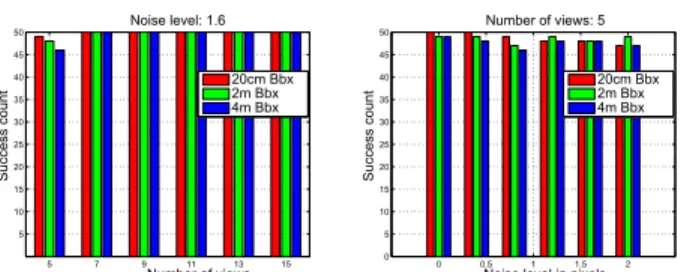
The median time taken for various experiments against the number of bounded cameras and image noise are shown in Figure 1. Similarly, Figure 2 shows the success count over 50 experiments. 2D-to-3D registration accuracy was measured by computing the 3D registration error of all 1000 reconstructed points to the scene. Measured 3D RMS reg-istration error is shown in Figure3. An experiment is as-sumed to be successful if it produces less than 0.1 3D er-ror. The estimated camera intrinsics and pose were com-pared against that of ground truth. The Euclidean projec-tion matrix of the first camera was recovered using PE1 = K1[R1 t1] = P1H−1. For the evaluation, error measurement
metrics forN number of experiments are defined as follows ∆f = $ N ! i=1 (α1 i−α)2+(βi1−β)2 N(α2+β2) , ∆R = $ N ! i=1 ||r1 i−r||2 3N , ∆uv = $ N ! i=1 (u1 i−u)2+(vi1−v)2 N(u2+v2) , ∆t = $ N ! i=1 ||t1 i−t||2 N(||t||2) ,
whereα1, β1represent two focal lengths, and(u1, v1) is the
principal point. r1is a vector obtained by stacking three ro-tation angles in degrees. These angles are obtained from R1 after enforcing its orthogonality. The corresponding vari-ables without subscript represent the ground truth. The er-rors in camera intrinsics and pose are shown in Figure4. The success, speed, and accuracy improve with the increase in number of views and decrease in the box size.
5 10 15 0 50 100 150 200 250 Number of views T ime in se co nd s Noise level: 2.0 20cm Bbx 2m Bbx 4m Bbx 0 0.5 1 1.5 2 0 50 100 150 200 250
Noise level in pixels
T ime in se co nd s Number of views: 7 20cm Bbx 2m Bbx 4m Bbx
Figure 1: Time vs. number of views and noise.
5 7 9 11 13 15 5 10 15 20 25 30 35 40 45 50 Number of views Su cce ss co un t Noise level: 1.6 20cm Bbx 2m Bbx 4m Bbx 0 0.5 1 1.5 2 0 5 10 15 20 25 30 35 40 45 50
Noise level in pixels
Su cce ss co un t Number of views: 5 20cm Bbx 2m Bbx 4m Bbx
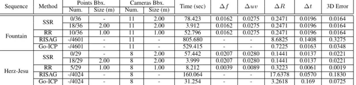
Sequence Method Points Bbx. Cameras Bbx. Time (sec) ∆f ∆uv ∆R ∆t 3D Error
Num. Size (m) Num. Size (m)
Fountain SSR 0/36 - 11 2.00 78.423 0.0162 0.0275 0.2471 0.0196 0.0164 18/36 2.00 11 2.00 3.912 0.0162 0.0275 0.2471 0.0196 0.0164 RR 10/36 1.00 11 1.00 52.796 0.0162 0.0275 0.2471 0.0196 0.0164 RISAG -/4601 - 11 - 805.680 - - 8.6825 0.1408 0.3275 Go-ICP -/4601 - 11 - 529.415 - - 0.7225 0.0163 0.0348 Herz-Jesu SSR 0/29 - 8 2.00 57.442 0.0207 0.0280 0.1441 0.0137 0.0221 18/29 2.00 8 2.00 3.999 0.0207 0.0280 0.1441 0.0137 0.0221 RR 5/29 1.00 8 1.00 8.212 0.0039 0.0089 0.3223 0.0061 0.0019 RISAG -/4024 - 8 - 160.064 - - 17.6378 0.0570 0.1830 Go-ICP -/4024 - 8 - 31.254 - - 3.2618 0.169 0.0725
Table 1: Four different methods with real data. Points Bbx.p/q means p number of points are bounded out of q sought.
5 10 15 0 0.001 0.002 0.003 0.004 0.005 0.006 0.007 0.008 0.009 0.01 Number of views 3D Err or Noise level: 1.2 20cm Bbx 2m Bbx 4m Bbx 0 0.5 1 1.5 2 0 0.001 0.002 0.003 0.004 0.005 0.006 0.007 0.008 0.009 0.01
Noise level in pixels
3D Err or Number of views: 7 20cm Bbx 2m Bbx 4m Bbx
Figure 3: Registration error vs. number of views and noise.
5 10 15 0 0.02 0.04 0.06 0.08 0.1 0.12 0.14 0.16 0.18 0.2 Number of views
Error in focal length (
∆ f) Noise level: 1.6 20cm Bbx 2m Bbx 4m Bbx 5 10 15 0 0.01 0.02 0.03 0.04 0.05 0.06 0.07 0.08 0.09 0.1 Number of views
Error in principal point (
∆ uv) Noise level: 1.6 20cm Bbx 2m Bbx 4m Bbx 5 10 15 0 0.5 1 1.5 2 2.5 3 3.5 4 4.5 5 Number of views Error in rotation ( ∆ R) Noise level: 0.8 20cm Bbx 2m Bbx 4m Bbx 5 10 15 0 0.01 0.02 0.03 0.04 0.05 0.06 0.07 0.08 0.09 0.1 Number of views Error in translation ( ∆ t) Noise level: 0.8 20cm Bbx 2m Bbx 4m Bbx
Figure 4: Intrinsic and pose errors vs. number of views.
Figure 5: Fountain: (left) 11 cameras 2m Bbx and scene, (right) estimated cameras in textured scene using SSR.
Real data: We tested our method with two real datasets: Fountain-P11 and Herz-Jesu-P8 (from [25]). These datasets consist, respectively, of 11 and 8 images of size3072×2048 captured by a moving camera ofα = 2759.5, β = 2764.2, u = 1520.7 and v = 1006.8, along with the laser scanned
Figure 6: Herz-Jesu: (left) matched 2D features with out-liers in red, (right) texture-mapped scene using RR.
3D scenes. Our results were compared against two meth-ods: RISAG [6] and Go-ICP [30]. RISAG requires met-ric reconstruction, hence works only for the calibrated case. Likewise, Go-ICP requires an Euclidean reconstruction, which was obtained by upgrading the metric reconstruc-tion using ground truth projecreconstruc-tion matrices. The metric re-construction was obtained using openMVG [15]. The re-sults obtained for all four methods are shown in Table1. For qualitative analysis, estimated projection matrices were used for texture mapping. The obtained results using our methods were very accurate. These are shown in Figures5
-6which also provide the results after further refinement us-ing [29]. Note that a small error in pose can significantly affect the texture mapping. For the Fountain sequence, both SSR and RR converged to the same solution. RR, however, converged to a better solution for Herz-Jesu.
5. Conclusion
We have presented a novel approach for registering two or more uncalibrated cameras to a 3D scanned scene. The proposed approach only assumes point correspondences across images. Our solution allows estimating the unknown projective transformation relating the cameras to the scene and establishing 2D-3D correspondences. A LMI frame-work was used to overcome the image-induced point trian-gulation requirement. Using this framework, we have de-rived triangulation-free LMI cheirality conditions and LMI constraints for establishing putative correspondences be-tween 3D boxes and 2D points. Two globally convergent al-gorithms, one exploiting the scene’s structure and the other concerned with robustness, have been presented.
Acknowledgments
This research has been funded by the International Project NRF-ANR DrAACaR: ANR-11-ISO3-0003.
References
[1] D. Aiger, N. J. Mitra, and D. Cohen-Or. 4-points congruent sets for robust surface registration. ACM Transactions on
Graphics, 27(3):85, 1–10, 2008.1
[2] S. Boyd and L. Vandenberghe. Convex Optimization.
Cam-bridge University Press, New York, NY, USA, 2004.3
[3] M. Chandraker, S. Agarwal, F. Kahl, D. Nister, and D. Krieg-man. Autocalibration via rank-constrained estimation of the absolute quadric. In IEEE Conference on Computer Vision
and Pattern Recognition (CVPR), 2007.2
[4] M. Chandraker, S. Agarwal, D. Kriegman, and S. Belongie. Globally optimal algorithms for stratified autocalibration. In-ternational Journal of Computer Vision (IJCV), pages 236–
254, November 2009.2
[5] S. Christy and R. Horaud. Iterative pose computation
from line correspondences. In Comput. Vis. Image Underst
(CVIU), pages 137–144, January 1999.1
[6] M. Corsini, M. Dellepiane, F. Ganovelli, R. Gherardi, A. Fusiello, and R. Scopigno. Fully automatic registration of image sets on approximate geometry. International Jour-nal of Computer Vision (IJCV), pages 91–111, March 2013.
1,8
[7] P. Finsler. Uber das vorkommen definiter und semidefiniter formen in scharen quadratischer formen. Comment. Math.
Helv., 9, pages 188–192, 1936/37.3
[8] A. Fusiello, A. Benedetti, M. Farenzena, and A. Busti. Glob-ally convergent autocalibration using interval analysis. IEEE Transactions on Pattern Analysis and Machine Intelligence
(PAMI), pages 1633–1638, December 2004.2
[9] A. Habed, D. Pani Paudel, C. Demonceaux, and D. Fofi. Ef-ficient pruning lmi conditions for branch-and-prune rank and chirality-constrained estimation of the dual absolute quadric. IEEE Conference on Computer Vision and Pattern
Recogni-tion (CVPR), pages 493–500, 2014.2
[10] R. I. Hartley. Chirality. International Journal of Computer
Vision (IJCV), pages 41–61, January 1998.2
[11] R. I. Hartley and A. Zisserman. Multiple View Geometry in Computer Vision. Cambridge University Press, second edition, 2004.2,5
[12] J. Knopp, J. Sivic, and T. Pajdla. Avoiding confusing features in place recognition. In European Conference on Computer
Vision (ECCV), pages 748–761, 2010.1
[13] L. Liu and I. Stamos. Automatic 3d to 2d registration for the photorealistic rendering of urban scenes. In IEEE Confer-ence on Computer Vision and Pattern Recognition (CVPR),
pages 137–143, 2005.1
[14] M. A. Lourakis and A. Argyros. SBA: A software package for generic sparse bundle adjustment. In ACM Trans. Math.
Software, pages 1–30, 2009.7
[15] P. Moulon, P. Monasse, and R. Marlet. Adaptive structure from motion with a contrario model estimation. In Asian
Conference on Computer Vision (ACCV), pages 257–270,
2013.8
[16] D. Nist´er. Untwisting a projective reconstruction. Interna-tional Journal of Computer Vision (IJCV), pages 165–183,
November 2004.2
[17] D. Nister, O. Naroditsky, and J. Bergen. Visual odometry. In IEEE Conference on Computer Vision and Pattern
Recogni-tion (CVPR), pages 652–659, 2004.2
[18] J. Oliensis and R. Hartley. Iterative extensions of the
sturm/triggs algorithm: Convergence and nonconvergence. IEEE Transactions on Pattern Analysis and Machine
Intelli-gence (PAMI), pages 2217–2233, December 2007.7
[19] D. P. Paudel, C. Demonceaux, A. Habed, and P. Vasseur. Lo-calization of 2d cameras in a known environment using di-rect 2d-3d registration. In IEEE International Conference on
Pattern Recognition (ICPR), pages 1–6, 2014.1
[20] M.-T. Pham, O. J. Woodford, F. Perbet, A. Maki, B. Stenger, and R. Cipolla. A new distance for scale-invariant 3d shape recognition and registration. In IEEE International
Confer-ence on Computer Vision (ICCV), pages 145–152, 2011.1
[21] V. Rabaud. Vincent’s Structure from Motion
Tool-box. http://vision.ucsd.edu/˜vrabaud/ toolbox/.7
[22] S. Ramalingam, S. Bouaziz, P. Sturm, and M. Brand. Geolo-calization using skylines from omni-images. In IEEE Inter-national Conference on Computer Vision Workshops (ICCV
Workshops), pages 23–30, 2009.1
[23] T. Sattler, B. Leibe, and L. Kobbelt. Fast image-based lo-calization using direct 2d-to-3d matching. In IEEE Interna-tional Conference on Computer Vision (ICCV), pages 667–
674, 2011.1
[24] D. Scaramuzza and F. Fraundorfer. Visual odometry, part i: The first 30 years and fundamentals. In IEEE ROBOTICS and AUTOMATION MAGAZINE, pages 80–92, December
2011.2
[25] C. Strecha, W. von Hansen, L. Van Gool, P. Fua, and U. Thoennessen. On benchmarking camera calibration and
multi-view stereo for high resolution imagery. In IEEE
Conference on Computer Vision and Pattern Recognition,
(CVPR), pages 1–8, 2008.8
[26] P. Sturm. Critical motion sequences for monocular
self-calibration and uncalibrated euclidean reconstruction. In
IEEE Conference on Computer Vision and Pattern Recog-nition (CVPR), pages 1100–1105, 1997.
[27] A. Taneja, L. Ballan, and M. Pollefeys. Registration of spher-ical panoramic images with cadastral 3d models. In
3DIM-PVT, pages 479–486, 2012.1
[28] B. Triggs, P. Mclauchlan, R. Hartley, and A. Fitzgibbon.
Bundle adjustment a modern synthesis. In Vision
Al-gorithms: Theory and Practice, LNCS, pages 298–375.
Springer Verlag, 2000.7
[29] P. Viola and W. M. Wells, III. Alignment by maximization of mutual information. International Journal of Computer
Vision (IJCV), pages 137–154, September 1997.1,8
[30] J. Yang, H. Li, and Y. Jia. Go-icp: Solving 3d registration ef-ficiently and globally optimally. In IEEE International Con-ference on Computer Vision (ICCV), pages 1457–1464,