COMPUTER SIMULATION OF RELATIVISTIC
MULTIRESONATOR CYLINDRICAL MAGNETRONS
by
Hei-Wai Chan
Chiping Chen
onald C. Davidson
February, 1990
This research was supported in part by SDIO/IST under the
managment of Harry Diamond Laboratories, in part by the
Department of Energy High Energy Physics Division, and
in part by the Naval Surface Warfare Center.
MULTIRESONATOR CYLINDRICAL MAGNETRONS
Hei-Wai Chan, Chiping Chen and Ronald C. Davidson Plasma Fusion Center
Massachusetts Institute of Technology Cambridge, MA 02139
ABSTRACT
The relativistic multiresonator magnetron is analyzed in cylindrical geometry, using the two-dimensional particle-in-cell simulation code MAGIC. Detailed comparisons are made between the simulation results and the experiments by Palevsky and Bekefi
(Phys. Fluids 22, 986 (1979)] using the A6 magnetron configura-tion. Within a constant scale factor, the computer simulations show a similar dependence of microwave power on magnetic field, with dominant excitations in the n and 2n modes. In the
preoscil-lation regime, the electron flow in the simupreoscil-lations differs sub-stantially from the ideal Brillouin flow model. In the nonlinear
regime, the saturation is dominated by the formation of spokes.
In relativistic magnetrons, 1-6 pulsed high-voltage diodes
(operating in the several hundred kV to MV range, say) are used to generate microwaves at gigawatt power levels. Although magnetrons are widely used as microwave sources, a fundamental understanding of the underlying interaction physics is still being developed,7 particularly in the nonlinear regime. Much of the theoretical challenge in describing multiresonator magnetron operation arises from the complexity introduced by the corrugated anode boundary8 and the fact that the electrons emitted from the cathode interact with the electromagnetic waves in the anode-cathode gap in a
highly nonlinear way. This is manifest through strong azimuthal bunching of the electrons and the formation of large-amplitude "spokes" in the electron density. In this regard, computer simulation studies9~1 1
provide a particularly valuable approach to analyze the interaction physics and nonlinear electrodynamics in magnetrons.
In this letter, we summarize recent computer simulations of the multiresonator A6 magnetron configuration using the two-dimensional (a/az - 0) particle-in-cell code MAGIC.12 The code includes cylindrical effects, and relativistic and electromagnetic effects in a fully self-consistent manner. Unlike previous com-puter simulations, the magnetron oscillations are excited from noise, i.e., without preinjection of a finite-amplitude rf signal or preferential excitation of 2n-mode or n-mode oscillations. In addition, the present simulations are carried out in cylindrical. rather than planar9'1 0 magnetic geometry. Figure 1 shows the
cross section of the A6 magnetron.3 The field-emission cathode is located at radius a - 1.58 cm. The inside radius of the anode block is b - 2.11 cm, and six vane-type resonators with outer
radius d - 4.11 cm are used, with angle * = 20* subtended by the resonators on axis. The applied magnetic field Bfaz ranges from 4-10 kG in typical operation.3 The axial length of the anode
block is L - 7.2 cm, and the operating voltage is 300-400 kV. For transverse electric (TE) excitations with &E perpendicular to BfeZ and SB parallel to B fz, the vacuum electric field pattern in Fig.
1 is such that 6
Ee
is in phase in adjacent resonators for the 2n mode, whereas 6Ee is out of phase in adjacent resonators for the n mode.In the simulations, Maxwell's equations and the particle orbit equations are solved relativistically and electromagnetically, using (typically) more than 3000 macroparticles and a nonuniform,
two-dimensional grid consisting of approximately 3000 cells. When a voltage VD(t) is applied across the diode in Fig. 1, the elec-trons are emitted from the cathode through a space-charge-limited emission process in which the instantaneous electric field normal to the cathode surface vanishes. The radial momenta of the
emitted electrons are randomly distributed from 0 to 0.02 mc. On the other hand, electrons are absorbed by the anode or cathode whenever they strike the surface. The simulations are carried out with one open resonator, which is modeled by a dispersive window placed along the dashed line in Fig. 1 at r - d - 4.11 cm. At the window, the boundary condition is such that most of the electro-magnetic wave energy is absorbed, while a small fraction of the wave energy is reflected back into the cavity.
A quasi-static model is used in the simulations to describe the high-voltage pulse applied to the diode. In such a model, the diode voltage is given by VD(t) - Z(t)V0
(t)/[Z
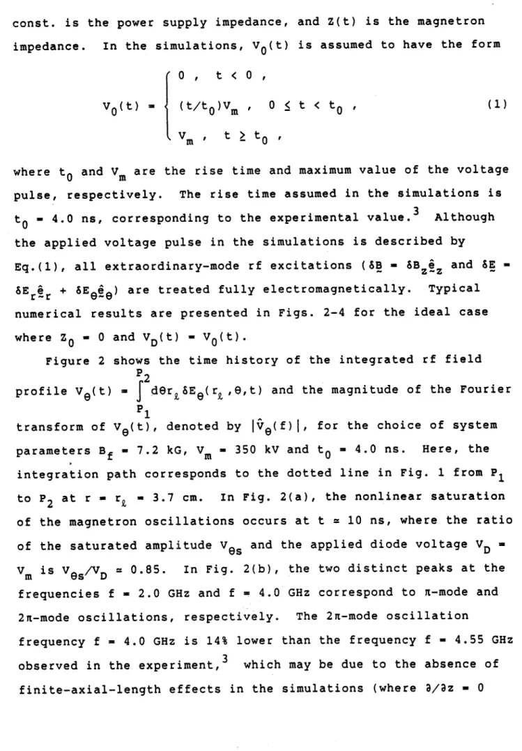
0 + Z(t)], where V0 (t) is the voltage pulse provided by the power supply, Z0-const. is the power supply impedance, and Z(t) is the magnetron impedance. In the simulations, Vo(t) is assumed to have the form
0
,t
<
0,
V0(t) - (t/t0
)Vm
0 t < to 'Vm , t > to '
where t0 and Vm are the rise time and maximum value of the voltage
pulse, respectively. The rise time assumed in the simulations is t0 - 4.0 ns, corresponding to the experimental value. Although the applied voltage pulse in the simulations is described by
Eq.(1), all extraordinary-mode rf excitations (SB -
&Bziz
and SE -SE rr + SEee)
are treated fully electromagnetically. Typical numerical results are presented in Figs. 2-4 for the ideal case where Z - 0 and VD(t) - V0(t).Figure 2 shows the time history of the integrated rf field p2
profile Ve(t) - Iderk SEe(rZ,9,t) and the magnitude of the Fourier p1
transform of Ve(t), denoted by
IVe(f)j,
for the choice of system parameters Bf - 7.2 kG, Vm - 350 kV and t0 - 4.0 ns. Here, theintegration path corresponds to the dotted line in Fig. 1 from P to P2 at r - r. - 3.7 cm. In Fig. 2(a), the nonlinear saturation of the magnetron oscillations occurs at t = 10 ns, where the ratio of the saturated amplitude Ves and the applied diode voltage VD ' Vm is VOs/VD = 0.85. In Fig. 2(b), the two distinct peaks at the
frequencies f - 2.0 GHz and f = 4.0 GHz correspond to n-mode and
2n-mode oscillations, respectively. The 2n-mode oscillation
frequency f - 4.0 GHz is 14% lower than the frequency f - 4.55 GHz observed in the experiment,3 which may be due to the absence of finite-axial-length effects in the simulations (where 8/3z - 0
is assumed). Although both excitations have nearly the same amplitude in Fig. 2(b), the (higher frequency) 2n mode delivers more rf power than the n mode.
By evaluating the area-integral of the outward Poynting flux (c/4n)gEaBz over the surface of the dispersive window at r - d
- 4.11 cm in Fig. 1, the peak rf power output in the simulations is calculated for various values of the applied magnetic field Bf. The dependence of the normalized rf power on magnetic field is shown in Fig. 3. Here, the dots correspond to the experimental values,3 and the triangles are obtained from the simulations with Z0 - 0. In Fig. 3, the normalization is chosen such that the max-imum values of the rf power in both the simulations and the exper-iment are equal to unity. The actual value of the maximum rf out-put per unit axial length in the simulations is 4.3 GW/m. For the A6 magnetron, with axial length L = 7.2 cm, this corresponds to P - 0.3 GW, which is somewhat less than the maximum rf power P - 0.45 GW measured in the experiment.3 (The values of power quoted here are rms values.) Apart from a constant scale factor,
it is evident from Fig. 3 that the simulations are in excellent agreement with the experimental results. The difference in scale factor may be due to the fact that a larger fraction of the rf power in the simulations is reflected back into the cavity, and
the effective Q-value in the simulations (Q - 100) is greater than in the experiment (Q - 20-40). As Bf is decreased below 6 kG, crossing the Hull cut-off curve2 at a diode voltage corresponding to VD - 350 kV, it is found that the 5n/3-mode (Z - 5) becomes the dominant rf excitation in the simulations.
In following the time evolution of the electron density n e(r,e,t) in the simulations, it is found that the profile for
2n
the average density, <ne>(r,t) - (2n)Vf dene(r,e,t), does not
0
2
resemble that corresponding to Brillouin flow, even at early times (t < 4ns, say). In particular, the profile for <ne>(r,t) decreases as r increases from r - a - .2.11 cm, and exhibits a
long tail extending beyond the layer radius rb calculated from an ideal Brillouin flow model.2 Although the azimuthal bunching of the electrons is relatively small for times up to 4 ns, by t ~ 6 ns the system begins to enter a nonlinear regime characterized by spoke formation. Highly developed spokes are evident in
Fig. 4(b) which shows density contour plots at t - 8 ns for the choice of system parameters Bf - 7.2 kG, Vm - 350 kV and t0 = 4 ns. The spokes rotate in the azimuthal direction as the system evolves, and there is current flow from the cathode to the anode. At saturation, which occurs at t = 10 ns, the time-averaged diode current per unit axial length is ID = 100 kA/m, and the amplitude
b
of the integrated rf field profile JdrSEr(r,9,t) is comparable with
a
the diode voltage VD =
Vm
- 350 kV.To summarize, with regard to the dependence of rf power on magnetic field, the simulation results are in excellent agreement with the experiment (within a constant scale factor). Also, in
terms of rf power output, the simulations confirm that the A6 magnetron oscillates preferentially in the 2n mode. In the
pre-oscillation regime, it is found that the electron flow differs substantially from Brillouin flow conditions. In the nonlinear regime, the saturation is dominated by the formation of spokes. The simulations also show that the magnetron performance and rf
power generation are degraded when the impedance z0 of the
external power supply is increased (in agreement with experiment) from the ideal value 0 - 0. As a general conclusion, based on the results of this paper, it is expected that the MAGIC simula-tion code can be used as an effective tool for experimental
magnetron design.
ACKNOWLEDGMENTS
The authors wish to thank George Bekefi, Shien Chi Chen and George Johnston for helpful discussions, and Bruce Goplen and Jim McDonald of Mission Research Corporation for consultations on the
MAGIC simulation code. This research was supported in part by SDIO/IST under the management of Harry Diamond Laboratories, in part by the Department of Energy High Energy Physics Division, and in part by the Naval Surface Warfare Center.
REFERENCES
1. J. Benford, in High-Power Microwave Sources, eds., V. Granatstein and I. Alexeff (Artech House, Boston, Massachusetts, 1987) p. 351. 2. R.C. Davidson, Physics of Nonneutral Plasmas (Addison-Wesley,
Reading, Massachusetts, 1990) Chapter 8.
3. A. Palevsky and G. Bekefi, Phys. Fluids 22, 986 (1979).
4. G. Bekefi and T.J. Orzechowski, Phys. Rev. Lett. 37, 379 (1976). 5. J. Benford, H.M. Sze, W. Woo, R.R. Smith, and B. Harteneck,
Phys. Rev. Lett. 62, 969 (1989).
6. A.G. Nokonov, I.M. Roife, Yu.M. Savel'ev, and V.I. Engel'ko, Sov. Tech. Phys. 32, 50 (1987).
7. Y.Y. Lau, in High-Power Microwave Sources, eds., V. Granatstein and I. Alexeff (Artech House, Boston, Massachusetts, 1987) p. 309. 8. H.S. Uhm, H.C. Chen, R.A. Stark, and H.E. Brandt, Proc. SPIE 1061,
170 (1989).
9. S.P. Yu, G.P. Kooyers and 0. Buneman, J. Appl. Phys. 36, 2550 (1965).
10. A. Palevsky, G. Bekefi, and A.T. Drobot, J. Appl. Phys. 52, 4938 (1981).
11. A. Palevsky, et al., in High-Power Beams, eds., H.J. Doucet and J.M. Buzzi (Ecole Polytechnique, Palaiseau, France, 1981) p. 861.
12. B. Goplen and J. McDonald, private communication (1989). The MAGIC simulation code was developed by researchers at Mission Research Corporation. The simulation results presented in this paper use the code version dated 1988.
FIGURE CAPTIONS
Fig. 1. Cross section of the A6 magnetron used in the computer
simulations.
The rf power is partially absorbed by the
dispersive window (dashed line) located at r - d-4.11 cm in the open resonator. An applied magnetic field B fz points out of the page.
Fig. 2. Shown in Fig. 2(a) is the time history of the
P2
integrated rf field profile Ve(t) - der,6EG(r2,e,t) P1
obtained in the simulations at radius r - rg - 3.7 cm in the open resonator for the choice of system param-eters Bf - 7.2 kG, Vm - 350 kV, t0 - 4.0 ns, and Z0 - 0.
Figure 2(b) shows the Fourier spectrum
IOe(f)]
of the signal in Fig. 2(a). The two distinct peaks at f -2.0 GHz and f - 4.0 GHz correspond to n-mode (t - 3) and 2n-mode (z - 6) oscillations, respectively.Fig. 3. Plots of the normalized peak rf power versus the
applied magnetic field B The dots correspond to the experimental results [A. Palevsky and G. Bekefi, Phys. Fluids 22, 986 (1979)], and the triangles correspond to the simulation results for Vm - 350 kV, t0 - 4.0 ns, and Z - 0.
Fig. 4. Density contour plots for n (r,e,t) obtained in the simulations at (a) t - 3.0 ns and (b) t - 8.0 ns for the same system parameters as in Fig. 2.
DISPERSIVE
WINDOW Fig. 1 d\b
r p0.4