Computational tools for modeling and measuring chromosome structure

Computational Tools for Modeling and Measuring

Chromosome Structure

by

Brian Christopher Ross

B.S., University of Maryland (1998)

Submitted to the Department of Physics

ARCHIVES

in partial fulfillment of the requirements for the degree of

Doctor of Philosophy in Physics

at the

MASSACHUSETTS INSTITUTE OF TECHNOLOGY

September 2012

@

Massachusetts Institute of Technology 2012. All rights reserved.

Author ...

-...

Department of Physics

June 11, 2012

Certified by..

Alexander van Oudenaarden

Professor

Thesis Supervisor

Certified by..

Accepted by ...

Paul Wiggins

Assistant Professor

Thesis Supervisor

...

Krishna Rajagopal

Associate Department Head for Education

Computational Tools for Modeling and Measuring

Chromosome Structure

by

Brian Christopher Ross

Submitted to the Department of Physics on June 11, 2012, in partial fulfillment of the

requirements for the degree of Doctor of Philosophy in Physics

Abstract

DNA conformation within cells has many important biological implications, but there

are challenges both in modeling DNA due to the need for specialized techniques, and experimentally since tracing out in vivo conformations is currently impossible. This thesis contributes two computational projects to these efforts. The first project is a set of online and offline calculators of conformational statistics using a variety of published and unpublished methods, addressing the current lack of DNA model-building tools intended for general use. The second project is a reconstructive analysis that could enable in vivo mapping of DNA conformation at high resolution with current experimental technology.

Thesis Supervisor: Alexander van Oudenaarden Title: Professor

Thesis Supervisor: Paul Wiggins Title: Assistant Professor

Acknowledgments

I want to acknowledge at the outset that much of the work presented here as my

own originated from conversations of my advisor, coworkers, thesis committee and even friends and family. In particular I am grateful to Hyun Jin Lee for help with microscopy, David Johnson for advice on the Traveling Salesman Problem, Henrik Vestermark for the use of his complex root solver in the Wormulator, and numerous coworkers for their helpful comments on both the oral and written parts of my thesis. Most of all I want to thank my research mentor Paul Wiggins for his patient guidance and consistent support of me throughout my graduate career. Paul gave me more credit than I deserved for many of his ideas, and trusted me with my own ideas more than I had any right to expect, for which I am enduringly grateful.

Finally, this thesis would have been much more difficult without the considerable patience and support from my friends and family. Longtime friends Pak and John helped me find a research group; many other friends gave critical support and advice during this time. My lovely girlfriend Yanghee endured many late evenings at the lab while I was working on my 3d-alignment method. A number of friends and family (from Maryland!) gave considerable moral support from the back rows at my thesis defense. My heartfelt thanks go out to everyone who supported and encouraged me throughout this long process.

Contents

1 Introduction

1.1 DNA mechanics ... ...

1.1.1 DNA mechanical parameters . . . .

1.1.2 Modeling DNA Conformation . . . .

1.1.3 Solution methods for conformational statistics 1.2 DNA conformation in vivo . . . . 1.3 Experimental techniques for measuring DNA conform

1.3.1 Chromosome conformation capture . . . .

1.3.2 Electron microscopy . . . . 1.3.3 Fluorescence microscopy . . . .

DNA labeling methods . . . .

Superresolution fluorescence microscopy . . .

2 End Statistics Calculator

2.1 End-to-end distribution . . . . 2.2 M ethod . . . .

2.2.1 Gaussian chain . . . . 2.2.2 Eigenfunction method . . . .

2.2.3 M onte Carlo . . . . 2.2.4 Harmonic approximation method . . . .

2.2.5 Finite-width delta function . . . .

2.3 Im plem entation . . . . 2.3.1 W eb interface . . . . ation

11

12 12 16 19 22 27 27

30

31 31

33

41 . . . . 42 . . . . 43 . . . . 43 . . . . 44 . . . . 46 . . . . 52 . . . . 54 . . . . 57 . . . . 57

2.3.2

Com m and-line tool . . . .

2.4

Results and Discussion . . . .

2.4.1

V alidation . . . .

2.4.2

Example: going beyond wormlike chain using cyclization data

2.5 Appendix A: Derivatives of the constraint functions . . . .

2.6 Appendix B: Converting p into a density in angular coordinates . . .

3 Measuring Chromosome Conformation In Vivo

3.1

Proposed experiment . . . .

3.2 Analysis: the 3D-alignment method . . . .

3.2.1 The partition function Z . . . .

3.2.2 Step 1: calculate Z . . . .

3.2.3 Step 2: adjust weighting factors . . . .

3.2.4 Connection to the Traveling Salesman Problem . . 3.2.5 General comments . . . . 3.3 Performance of 3D-alignment algorithm on simulated data 3.4 Conclusions and Outlook . . . .

58

59

59

62

65

68

71

. . . .

72

. . . .

74

. . . .

76

. . . .

78

. . . .

80

. . . .

84

. . . .

85

. . . .

86

. . . .

93

List of Figures

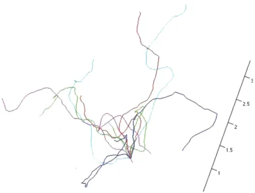
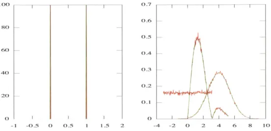
2-1 Monte Carlo-generated conformations . . . . 2-2 Monte Carlo sampling of single-segment distributions . . . .

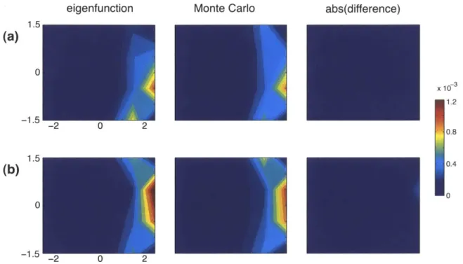
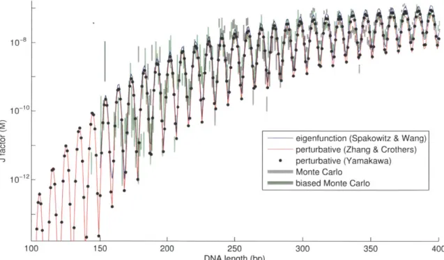
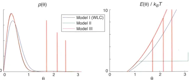
2-3 Comparison of distributions calculated by eigenfunction and Monte C arlo m ethods . . . . 2-4 Comparison of methods for calculating DNA cyclization rates . . . . 2-5 Cyclization of nicked DNA: energy functions of different models . . . 2-6 Cyclization of nicked DNA: energy-minimized kinked and unkinked

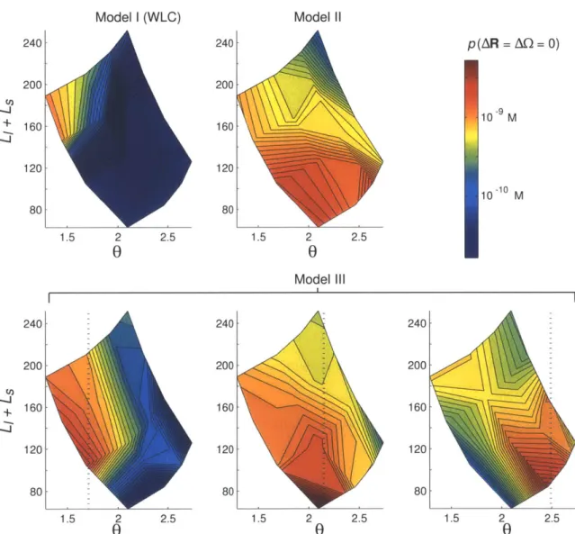
contours . .... ... .. . . .. . . . ... . . . .. ... 2-7 Cyclization of nicked DNA: cyclization frequencies . . . .

3-1 3-2

3-3

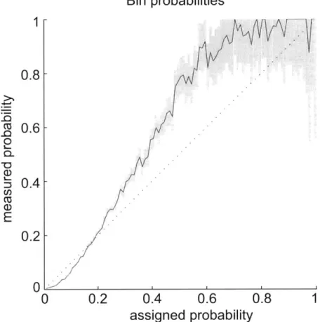
3-4 3-5 3-6

Quality of mapping probabilities . . . .

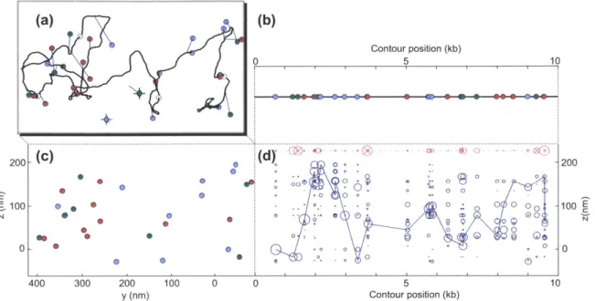
Comparison with control mappings . . . . Mapping of simulated 10 kb conformation . . . .

Obtaining discrete conformations . . . .

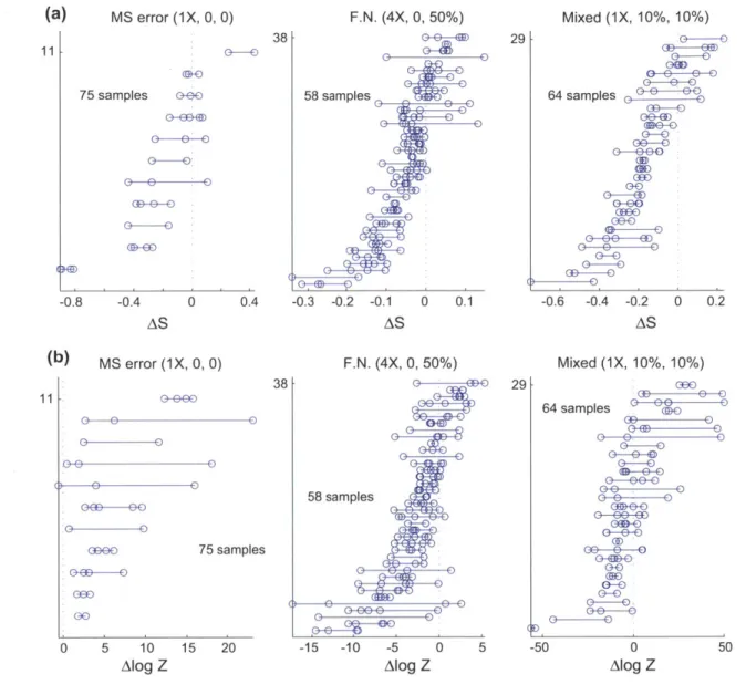
Information recovery and experimental error of 3D 10 Information recovery from simulated conformations .

kb conformations 47

60

61 62 63 64 66 88

90

92 93 94 95

Chapter 1

Introduction

The goal of structural biology is to build an engineering blueprint of an organism that catalogs all of its molecular parts, where they reside and how they fit together to form a cell. Of all these molecules, none is more famous or (arguably) more important than the double strands of DNA called chromosomes whose base-pair sequences control the cell. Owing to the central role of DNA and the accumulating lines of evidence that

DNA structure plays a large factor in many biological processes, a major research

effort is now devoted to understanding how chromosomes are arranged inside of the cell. The importance of this effort was captured in the closing paragraph of a recent commentary on epigenomics[7], which christened the task of uncovering chromosome structure the 'Fourth Era' in the genomics revolution.

The sheer size of a chromosome gives it a structure unlike that of any other molecule. A single chromosome can sprawl from one end of its cell to the other

a thousand times, forming an unfathomable tangle that is apparently organized in biologically important ways. Modeling this enormous and complex structure is com-plicated by the fact that the small-scale mechanics are poorly understood, and that a wide range of length and energy scales are important for various biological pro-cesses. Experimentally photographing the structure of a chromosome in a single cell is quite impossible with current technology, although coarse-grained and cell-averaged structural data are now becoming available.

chromosome structure. The first of these, called the 'Wormulator', bundles a suite

of methods for calculating conformational statistics into a usable modeling tool for

the scientific community. Chapter 2 describes the Wormulator and demonstrates how

it can be applied to refine models of DNA bending. In Chapter 3 we propose an

experiment that could obtain extended high-resolution, single-cell conformations of

DNA. The proposed experiment requires a '3d-alignment' data analysis which we

demonstrate with our second tool.

The remainder of Chapter 1 briefly reviews the current state of knowledge of

DNA mechanics, the in vivo conformation of chromosomes, and relevant experimental

techniques with an emphasis on super-resolution fluorescence imaging.

1.1

DNA mechanics

A general goal of DNA structure models is to determine the free energy required

to impose certain conformational constraints on the DNA molecule. For example,

the cell may wish to bring together a gene and an enhancer, or wrap 150 base pairs

around a nucleosome, or supercoil a topological domain. These activities are typical

of those involved in chromosome packaging and segregation, gene regulation and other

essential cellular activities. The energetics of these processes help determine when and

to what extent they happen in a live cell, and those energetics are in turn determined

by basic mechanical properties of DNA.

1.1.1

DNA mechanical parameters

The starting point for any model of large-scale chromosome structure is a fine-scale

DNA model which specifies mechanical properties such as stiffness. Measurements of

these properties have typically fallen into two classes: those related to the consecutive

base pairs that form a dinucleotide step, and bulk properties such as the persistence

length that average over many bases.

A standard reference frame has been developed[31, 101] for specifying the

along the major groove, the y axis runs along the sequence strand, and z is defined

by x x y. Translations along x, y and z are called shift, slide and rise respectively; rotations about those axes are tilt, roll and twist respectively. In accordance with these definitions, both the mean values and variances of each of these six variables have been determined between each possible pair of base sequences, based on X-ray crystallographic structures of DNA-protein complexes[102]. The mean values deter-mine the unstressed conformation of a DNA contour, while the variances deterdeter-mine the stiffnesses in various degrees of freedom. An alternative convention is to define the base steps relative to a helical axis rather than a body-fixed axis. A full description of a base pair involves the relative position and orientation of one of the two bases with respect to the other: these translations and rotations are called shear, stretch, stagger, buckle, propeller, and opening.

Over the span of many subunits, any relaxed polymer of identical subunits takes the shape of a helix (or, in limiting cases, a line or a circle). Coarse-grained descrip-tions of DNA describe the mechanics of DNA in terms of the rate of bending of, and twisting about, the helical axis, rather than the translations and rotations of individ-ual subunits. The mean bend angle of a stretch of DNA about any perpendicular axis is zero because the helicity makes the bending isotropic (i.e. it is as likely to bend left as right, forwards or backwards). However, the mean twist is nonzero: relaxed

DNA twists in the right-handed sense about its helical axis on average once per every 10.5 base pairs. Over- and under-twisting are referred to as positive and negative

supercoiling respectively.

In a thermal environment the bending and twisting profile of a polymer will differ from that of the unstressed conformation, depending on the polymer stiffness and temperature of the thermal bath. The expected deviations in bending and twisting are parametrized by the bending and twisting persistence lengths. The mean dot product of the helical axis vectors between two loci decays exponentially with the interlocus spacing, and the length scale for this decay is the (bending) persistence length. Likewise the twist persistence length determines the mean decay of corre-lations in the rotation angle about the tangent, after having adjusted for the mean

twist. By convention the term 'persistence length' refers to the bending persistence

length.

The bending persistence length of double-stranded DNA has been experimentally

measured using many methods, with the consensus being that it is at about 50 nm

in vitro (reviewed in [52]). An early technique for measuring the bending persistence

length relied on the absorbance of a DNA solution where the DNA molecules had

been aligned by an electric field, then allowed to relax diffusively for a short time.

The degree of relaxation was then measured by measuring the opacity of the solution

to light polarized along the electric field. The relaxation rate in turn depends on

the stiffness of the molecule[147], yielding a persistence length[111]. Translational

diffusion can also be used to measure the persistence length. The persistence length

of single-stranded DNA at electrophoresis conditions was measured to be about 4

nm[146] using fluorescence recovery after photobleaching (FRAP), in which a solution

of fluorescently-labeled DNA is bleached by overexposure within a small region of the

solution, and the subsequent rate of recovery of fluorescence in that region is measured

to determine the diffusion rate of the DNA and indirectly the persistence length.

A technique for measuring DNA persistence length that is very sensitive to

highly-bent conformations is to measure the cyclization rate of short

(~

100 base pair)

oligonucleotides[131]. In this assay a dilute mixture of DNA is ligated, and the ratio

of intermolecular ligations to cyclizations gives the effective concentration of one end

relative to the other, which is called the J factor. From the J factor one can determine

the persistence length[161, 129]. The single-stranded DNA persistence length has been

measured using the proximity of the two ends, rather than cyclization which requires

strict matching of the two ends' orientations[92]. The single-stranded measurement

used F6rster resonance energy transfer (FRET), a fluorescence method whereby an

excited donor fluorophore on one end of the DNA transfers some of its energy to

an acceptor fluorophore on the other end, causing the latter to emit a photon. The

persistence length of single-stranded DNA was measured by FRET to be only 1.25

-

3

nm, depending on NaCl concentration, which indicates that the mutual support of the

complementary strands contributes considerably to the stiffness of double-stranded

DNA.

The stiffness of DNA has been probed more directly by pulling on it with optical tweezers[6, 154], in a setup in which one end of a DNA oligo is fixed to a surface while the other is attached to a transparent bead in an optical trap. The optical trap is a converging beam of light refracts through, and thereby imparts momentum to, the bead thus creating a force on the bead towards the focus of the beam. The displace-ment of the bead from the center of the beam indicates a net external force which can be determined from the magnitude of the displacement. From the force required to pull the two ends of a given length of DNA to a given separation distance, one can obtain the persistence length[100, 85]. There are non-optical ways of stretching

DNA as well. One experiment fixed one end of a DNA oligo, pulled the other end

with an atomic force microscope, and inferred the pulling force from the deflection of the tip[117]. Finally, bending-force measurements were made by pulling DNA oligos between a bead caught in a pipette and the tip of a perpendicular optical fiber; the displacement of the fiber was imprinted on an optical beam passing through it and recorded by a photodetector[25].

Electron microscopy has also been used to measure the DNA persistence length

by directly imaging DNA contours in two[40] and three[8] dimensions. By measuring

the tangents along the contour at various locations on a DNA sample, and tracing out the contour distances between those points, one can measure the decay constant in tangent correlations that defines the bending persistence length. A correction has to be made for dimensionality: DNA prepared on electron microscope slides that has equilibrated in two dimensions will have a larger persistence length by a factor of 2 than a three-dimensional contour, although the extent to which the samples are truly two-dimensional on a microscope slide can be unclear.

The twist persistence length It has been estimated in a number of ways. One type of measurement exploits the fact that fluorophores have nonisotropic polarization cross sections for excitation and emission; exciting fluorescently labeled DNA with polarized light and measuring the rate at which the polarization of emission decays to isotropic can be used to find the twist persistence length[65] (this method can

also measure bending stiffness). Another estimate[90] of the twist persistence length comes from fixing one end of a stretch of DNA, attaching a magnetic bead to the other end, rotating the bead by an external magnet and measuring the fluctuations of the bead at different torsional angles[143]: this measurement yielded it = 120 nm.

Other measurement methods compare the cyclization efficiency of DNA oligos differ-ing slightly in length[130], or the efficiency of cyclizdiffer-ing at various linkdiffer-ing numbers[29]. The various estimates of l are generally close to 100 nm.

1.1.2

Modeling DNA Conformation

The most accurate computational models of molecules are those that compute the trajectories of each bonded atom in the molecule from first principles, a technique which is called molecular dynamics (MD)[12]. Using MD to model DNA requires simulation not just of the DNA oligonucleotide but also of the surrounding solution consisting of water molecules and ions, since the solvent interacts strongly with the negatively-charged DNA backbone. In order to initialize a MD simulation the system is first brought to a minimum-energy state close to a known structural conformation of the system, then evolved in time until the initial state is forgotten. MD can resolve dynamical processes such as the structural transition from A-form DNA to B-form[19], equilibrium conformational properties such as mean bending between base pairs[165], and mechanical properties that depend on thermal fluctuations such as the bending and twisting stiffnesses[77, 99, 108]. Simulations by MD usually require a lot of computation time.

Coarse-grained models of DNA omit the details of the individual atoms, and instead resolve the contour of either the helix or the helical axis. These models fall into two classes: discrete and continuous[160]. In a discrete model the contour is represented as a series of rigid line segments connected by joints (the segments may or may not correspond to individual base pairs). In a continuous model the DNA contour is represented as a mathematically smooth curve in space. Within these categories the various models differ in how rotations and twists occur between adjacent segments along the contour. Some models treat only bending, by parametrizing each segment

with a tangent vector pointing along the contour; other models use both a tangent vector and a normal vector which establishes a twist sense. Different models treat polymers as inextensible by fixing each segment length, or extensible in which the segment length varies according to some distribution. A final distinction is between models that consider non-adjacent interactions between segments, such as excluded volume, and those that ignore them which makes most analyses much more tractable. Excluded volume is often ignorable if either: the interactions between segments are either very rare, or (paradoxically) if they are so common that very long range, isotropic interactions dominate[33]. Models that ignore excluded volume are called phantom-chain models.

Common discrete polymer models are the jointed chain model, the freely-rotating chain model, and the rotational isomeric state model[160], in order of in-creasing complexity. In the freely-jointed chain model each segment is free to rotate arbitrarily with no energy penalty with respect to its neighbors. In the freely-rotating chain model the bend angle

0

of each joint is fixed but the direction of bending

#

may freely take any value from 0 to 2-r. The rotational isomeric state model fixes not only

0

but also

#

to one or several values. Both of these models deal with inextensible polymers. Unlike the first two models the rotational isomeric state model cannot ignore twisting, since the twist angle defines the allowed bending directions between each segment.

A popular continuous polymer model is the wormlike chain model (WLC)[75],

in which the bending energy is given by the function E = (lp/2)

f(du/dl)

2dl. The WLC can be understood as the limit of a discrete polymer divided into infinitesimal segments connected by infinitely stiff springs, where the limits are taken so that the overall bending scale is the persistence length

lp.

The most common wormlike chain models are isotropic in bending and may or may not deal with twist. An extended model called the helical wormlike chain[160] includes twist and allows for a mean bending angle relative to the twist vector, so that the minimum energy configuration

is a helix rather than a straight line.

de-viations of the DNA contour from the minimum-energy configuration, but are not necessarily correct for sharply bent or twisted contours. Indeed, sharp bends or kinks may form in DNA at a much higher rate than a linear model would predict[24], al-though this is controversial [35]. That kinks would form more easily than linear theory predicts is perhaps not surprising given that DNA is often very sharply bent in vivo. One way to incorporate kinking into polymer models is to assume a smooth worm-like chain contour with a quadratic bending energy that is punctuated by a number of kinks, where each kink has an energetic cost that is independent of, or weakly dependent on, bending angle[162, 110, 115, 157, 156].

Over many persistence lengths a polymer effectively performs a random walk in steps of the Kuhn length aK _{21p, resulting in a near-Gaussian probability} distri-bution between the two ends. This fact inspires the Gaussian chain model, which imagines replacing a length-L polymer having persistence length

l

with a polymer having length L/a and persistence length

la

while taking the limit a -+ 0, such that the end-to-end distribution becomes exactly Gaussian whose decay constant converges to a finite value. The Gaussian chain model predicts only the relative displacements of the two ends, not the intermediate contour. The relative twist between the two ends is completely uniform (because the length is effectively infinite), and the probability distribution for the end-to-end displacement R is determined only be the separation distance

R

by the formula

p(R)

=

(a/7)

3/2 _exp

_(-aR

2_{), where a}

_{= 3/IL}

_{for the freely}

jointed chain

(I

_{is the segment length) and a = 3/aKL for a wormlike chain.}

One structural phenomenon of DNA in vivo for which excluded volume cannot be neglected is supercoiling. A supercoiled polymer is subjected to torsion, which is relieved by a mixture of twist and writhe (coiled bending). Analytically, it is possible to impose some small amount of twist and writhe within the framework of phantom chain models[15] as long the configuration is not destabilized much from the unstressed conformation. However, strong supercoiling causes forward-and-back excursions of the contour called plectonemes, in which the forward and backwards halves coil around and support one another. A proper model of a plectoneme thus requires modeling of the support interactions between nonadjacent parts of the polymer; generally this is

done numerically (for example see [17]).

1.1.3

Solution methods for conformational statistics

Starting from a given model of the local mechanical properties of a polymer, a variety of analytical and computational techniques can generate statistics relating to large-scale conformation. These statistics relate to biologically-important quantities such as the rates of DNA looping and cyclization (end-to-end joining of an oligo with matching tangents and twists), and the free energies of supercoiling, compacting and packaging DNA. Each calculational technique is generally tailored to a certain DNA model or class of models, either discrete or continuous, and works best in a certain regime of DNA length (relative to the persistence length) and the degree of bending and twisting (relative to thermal fluctuations).

The conformational statistic we will be most concerned with is the end-to-end probability distribution of a DNA segment. This is the probability density for find-ing the two ends of a length-L polymer segment in a given relative position and/or orientation. For example, suppose we would like to know the free-energy cost paid

by a DNA-bridging protein when it binds two locations on the DNA and holds them

together. If, for simplicity, we ignore crowding effects between different parts of the polymer (as we will do consistently here), then the free-energy penalty is entirely due to the fact that the protein restricts the allowed configurations of the intervening segment between the two binding sites; the remainder of the polymer does not affect the free energy and can thus be ignored. Specifically, we can find the free energy penalty by integrating the length-L end-to-end distribution over the positions and orientations that satisfy the boundary conditions of the protein's binding sites. The particular distribution of interest depends on the boundary conditions. For a rigid bridging protein, the two bound spots are essentially fixed relative to one another, and we need to work with a probability density that accounts for both relative po-sition and orientation. If a sufficiently flexible linker in the protein connects its two binding sites, then the relative orientation may be considered free, so it is simpler to integrate, up to the maximum spacing of the linker length, a reduced distribution

that is only a function of the separation distance of the two ends.

A very general method for obtaining statistics of discrete conformations is Monte

Carlo sampling. A Monte Carlo algorithm draws representative values for the free parameters of a contour (for example the bending and twisting angle between each pair of consecutive segments) based on some prior distribution that comes from the

DNA model being used, then generates conformations using those parameters and

uses those conformations to obtain the statistics of interest. Monte Carlo can ac-commodate very general polymer models, which may or may not involve extension of the contour, nonharmonic energy functions, sequence dependence along the contour, etc.. Since the common form of Monte Carlo samples conformations in proportion to their occurrence in a random thermal environment, and because computational sampling is usually much slower than the thermal sampling performed by a physical system, it can be difficult to sample very rare conformations, implying that Monte Carlo generally works best in the low-energy regime.

A variant of Monte Carlo, called the Metropolis method[89], constructs

confor-mations by a series of iterative perturbations on a starting conformation. The con-formation at each iterative step n is subjected to some permutation in an attempt to generate the next conformation at step n + 1. The new conformation is accepted if: the new conformation satisfies any user-imposed constraints; and if the ratio of statis-tical weights Pn+1/p, is either greater than one or greater than a randomly-generated number on the uniform interval

[0,

1], a rule which ensures the proper weighting of

samples. If any of these tests fails then the n + ith conformation must be resampled using a different permutation of the conformation at step n. Only a well-separated subset of conformations form the sample set, in order to ensure that the samples are relatively uncorrelated. Metropolis sampling is good for enforcing constraints that would rarely be satisfied by the basic Monte Carlo method.

Several techniques have been developed to deal with conformations of discrete polymers that are rare because they are sharply bent or twisted relative to the size of thermal fluctuations. These methods take advantage of the fact that such con-formations tend to be sharply clustered around the minimum-energy conformation

that satisfies a set of constraints. The general method is to find this minimum-energy conformation and calculate the end statistics by perturbation. The original method

by Zhang and Crothers[166] took a quadratic expansion in the energy about the

minimum energy configuration, and integrated them exactly along with the Fourier-transformed constraint functions; this method can accommodate sequence-dependent models since every joint is accounted for separately. A later technique by Wilson and coworkers[158] calculates the normal modes of the polymer about the minimum-energy conformation, subject to endpoint constraints, and integrates over the ampli-tudes of these modes. The normal-mode analysis is similar to an earlier approximate analytical treatment of cyclized DNA[129]. The methods of Zhang and Crothers dis-agreed somewhat with those of Wilson et. al., and although the latter claim to be in better agreement with earlier work[129] it is still unclear which is the more accurate. Both techniques fail outside of the high-bending regime.

A transfer matrix technique exists[163, 164, 162] that can calculate end statistics

in both high- and low-energy regimes, using a formalism that discretizes not only the chain contour but also the orientation of each segment. Each element of a transfer matrix T.f~(klj contains the statistical weight for evolving segment n at orientation

i

to segment n + 1 at orientation

j;

each matrix also absorbs the Fourier-transformed

positional end constraint as denoted by the wavenumber k. Any bending and twisting energy functions may be used, and by interposing different transfer matrices sequence-dependent models can be accommodated.

The end statistics of continuous model polymers can be calculated using formal methods that were originally developed for quantum mechanics. The partition func-tion that integrates over the bending and twisting angles along the DNA length is formally equivalent (up to an imaginary factor) with a path integral over the rotations of a quantum spinor in time. Converting the path integral of the orientation-only par-tition function into a Schr6dinger equation allows one to borrow the solution from quantum mechanics, which is an eigenbasis of Wigner functions[160]. The perturba-tive method of Spakowitz[139, 140, 138, 88] extends the method to include a relaperturba-tive position constraint, by adding off-diagonal terms to the orientation-only Hamiltonian,

which a perturbative analysis reduces to a solution in terms of continued fractions

weighting the eigenstates. This work has been extended beyond the wormlike chain

by Wiggins et. al., who developed the continuous kinkable wormlike chain model[157]

in which each kink pays a fixed energy penalty regardless of the discontinuous bend

angle it imposes, and the subelastic chain model[156] which incorporates an energy

that is first-order in the bend angle.

1.2

DNA conformation in vivo

In all organisms the physical length of genetic material (~ 0.3 - 300 mm) greatly

exceeds the dimensions of the cell (- 1 - 100pm). Compacting and arranging the

genetic material is a necessary chore that every cell must perform. Furthermore, the

genetic material must be faithfully untangled and segregated with each cell division

cycle. Maintaining such a lengthy genome is a necessary hassle, but many cells (mostly

eukaryotes) exploit the rich palette of possible conformational states to aid various

cellular processes.

Cells compact their DNA using a variety of DNA-condensing proteins[83]. In

bac-teria, H-NS and Lrp are proteins containing both DNA-binding domains and

dimer-ization (H-NS) or multimerdimer-ization (Lrp) domains; these associate in vivo to form protein complexes with multiple DNA-binding sites that may help compact the DNA

by bringing distal regions together. Lrp forms either octomeric or hexadecameric

complexes depending on the leucine concentration, indicating that this amino acid sensor may transduce a chemical signal into a physical rearrangement of the chromo-some. Various structural maintenance of chromosome (SMC) proteins such as MukB in

E.

coli are believed to form dimers that loop around DNA, tying multiple DNA strands together either within a single dimer or through the association of dimers into multimeric 'rosettes'. The proteins IHF, HA and Fis introduce bends into the

DNA, leading to an effective shortening of the persistence length and compaction of

the chromosome. Fis may also help compact the genome by multimerizing.

chromo-somes at a variety of scales. Electron microscopy of extracted bacterial chromochromo-somes reveals them as supercoiled loops emanating from a dense central core[72, 112] likely composed of RNA and protein, although the exact picture depends strongly on the preparation. The most recent estimate[112] gives the loop lengths roughly an ex-ponential distribution with a mean of 10 kb. Experiments measuring the level of supercoiling in different parts of the genome suggest that the chromosome is divided into topological domains, where the level of supercoiling equilibrates throughout each domain but cannot propagate beyond the two flanking domain walls. The size of the topological domains in E. coli was originally estimated at 100 kb [72], but newer studies have argued for smaller domains of 10 kb [112], consistent with the sizes of the

DNA loops. On larger scales, recombination experiments[149] and FISH[96] suggest

that the E. coli genome may organize into 2-4 larger 'macrodomain' structures. On the global scale, many prokaryotic genomes seem to be arranged in an orderly way down the length of the cell. For example, the E. co/i genome is packaged linearly along the long axis of the cell, with the origin located at mid-cell and the two arms spreading towards opposite poles[155]. Because the E. coli genomne seems to be a closed loop, as are most bacterial chromosomes (though there is some controversy about this-see [9]), it seems that the terminus region of the genome must stretch tightly from one end of the cell to the other in order to connect the two arms, although this has not yet been seen directly. The arrangement of the Caulobacter genome is also linear at the global scale[152], except that the terminus is at one cell pole, the origin of replication is at the other, and the two arms between origin and terminus are both stretched in parallel along the full length of the cell. Less is known about radial positioning; one very recent study found that loci encoding membrane proteins in the E. coli genome are apparently pulled to the cell periphery when those genes are expressed[81], affecting the positioning of loci up to 100 kb away.

In both E. co/i and Caulobacter, newly-replicated genomic loci are segregated rapidly to their appropriate locations within the two daughter clls[152]. There are two replisomes (replication machines) per parent chromosome in E. coli. Both repli-somes begin their work at the middle of the parent cell where the origin of replication

is located, but soon thereafter follow the two replication forks out towards the

op-posite poles, then come back again to the center of the parent cell as the replication forks meet again at the terminus[116].

The linear arrangement of DNA in

F.

coli[155] and Caulobacter[152] suggests that in these organisms, and perhaps in the majority of prokaryotes, genetic material is simply arranged for convenient packaging and not organized for higher-order control over processes such as transcription. However, nature does exploit the fact that gene copy number and therefore transcription levels correlate with genomic position in dividing cells[137], since origin-proximal regions are replicated first and are therefore present in higher numbers during DNA replication. Genomic position in turn corre-lates with physical position along the long axis of the cell in many species[155, 1521.

Genomic compaction in eukaryotes relies largely on histone proteins which form oc-tameric spool-like complexes called nucleosomes[74]. Each nucleosome tightly wraps 146 base pairs of supercoiled DNA around its outside, corresponding to about l3

4

complete turns of the DNA around the nucleosome particle. Nucleosomes are sepa-rated by 'linker' stretches of DNA of random lengths averaging around 50 base pairs: due to their tight packing the mass of nucleosomes approximately equals the mass of DNA. Protruding tails from the individual histone proteins interact with the tails of other nucleosome particles, causing them to aggregate into higher-order structures and leading to compaction of the DNA.

Nucleosome-bound DNA, called chromatin, has different mechanical properties from bare DNA. It seems that short lengths of chromatin are more flexible than bare DNA[118]. At longer lengths it is believed that nucleosomes bind one another and arrange the DNA into a thicker fiber whose structure is still controversial. The traditional view is that nucleosomes package DNA into a regular '30-nm fiber'[26], although newer measurements suggest that the fiber may under some conditions

be-come _{about 50% thicker[120], and others indicate that such a fiber is nonexistent[37]}

which would imply a disordered arrangement of eukaryotic DNA.

Nucleosome-bound DNA exists in one of two forms: transcriptionally-active eu-chromatin, and repressed heterochromatin. While both forms of chromatin may fold

into a 30-nm fiber, heterochromatin is further compacted on larger scales[45] causing steric exclusion of DNA-binding factors required for transcription and thus preventing expression of genes within that region. Chemical modifications to the nucleosomes nucleate heterochromatic regions, which then spread along open DNA through the action of proteins such those encoded by the silent information regulator (Sir) genes in yeast. The boundaries between euchromatic and heterochromatic regions are de-marcated by 'boundary elements' that in some or all cases are associated with CCTF and cohesin[51]. Cohesin is a member of the SMC protein family, and like MukB is believed to dimerize to form a ring that can ensnare several strands of DNA at a time, thereby bringing them together[64]. It seems likely that CCTF recruits co-hesin to boundary elements, and that coco-hesin in turn somehow prevents the spread

of heterochromatin.

Cohesin also plays a role in activating the transcription of eukaryotic genes by altering the conformation of the chromosome. Transcription initiation requires the assembly of a number of protein factors, some of which bind at the gene promoter and some of which bind to distal enhancer elements which can be up to hundreds of kilobases away. A protein complex containing both cohesin and the mediator complex forms contacts between enhancer elements and gene promoters[97, 71] in order to activate transcription. Other elements termed insulators block the action of enhancers. Insulators are associated with CTCF and cohesin, and it is thought that the cohesin complex tethers DNA in a way that blocks the enhancers from looping over to their target promoters[1]. Cohesin thus upregulates or downregulates gene expression, depending on which protein partners it associates with.

Transcribed genomic loci frequently associate in the cell in DNA-protein complexes called 'transcription factories'[68, 103]. Actively dividing HeLa cells are estimated to have several thousand transcription factories at any given time. It is not clear whether the colocalization of genes has a purpose or is just a byproduct of active transcription, but a recent experiment[79] discovered numerous interacting promoters in human cells whose gene expression levels were both correlated and affected by the presence of the nearby promoters. The authors suggested that the physical coupling of genes during

transcription is involved in the combinatorial regulation of gene expression.

In some cases the positioning of genomic loci relative to the nuclear envelope coor-dinates gene expression and DNA maintenance. Repressed genes are often associated with the nuclear envelope in yeast[1] or the nuclear lamina in mammalian cells[46]. In yeast, association with the nuclear pores can, paradoxically, increase the expres-sion levels of certain genes[1], and damaged DNA has been shown to be recruited to

nuclear pores for repair[931.

Recombination, both intentional and accidental, is influenced by the mutual acces-sibility of the recombining genomic regions. Examples of intentional recombination in mammals are the generation of unique immunoglobulins (which include antibodies) in mammalian B cells, and of T cell receptors in T cells, in which recombination involves the looping of the recombinant regions[70]. Unintentional, mutagenic recombination usually occurs between genomic regions that are nearby in physical space[87], a fact which likely implicates DNA conformation in a cell's predisposition to certain types of cancer.

Eukaryotic chromosomes are organized into megabase-scale domains bounded by CTCF-enriched boundary elements[32, 98]. A given locus associates much more of-ten with chromatin within its own domain than loci residing outside the domain, and gene expression level is strongly correlated within each domain. On the largest scales, individual interphase chromosomes of higher eukaryotes tend to arrange in distinct, non-overlapping chromosomal territories[87], although the territory occupied by each chromosome depends partly on cell type and state and varies considerably between cells. During mitosis and meiosis the chromosomes condense with the aid of con-densins, which are members of the SMC protein and operate similarly to cohesin. Kinetochore motors walking along microtubule spindles partition daughter chromo-somes between dividing daughter cells. The large-scale organization of interphase chromosomes after mitosis is somewhat consistent between cells, but the mechanisms behind, and significance of, this organization are still unknown.

1.3

Experimental techniques for measuring DNA

conformation

A number of experiments have probed conformation in an indirect way, without

re-solving explicit genomic interactions or positions. Information about the compactness of DNA comes from studying the permeability of different cellular regions; high per-meability presumably corresponds to low DNA packing density and vice versa. The permeability can be mapped out directly on the micrometer scale by measuring the mobility of diffusing fluorescent molecules using pair-correlation analysis[63]. An-other method of probing cellular permeability is to measure the frequency with which transposons jump or copy to various genomic loci; this maps density as a function of genomic position rather than density as a function of spatial position. A num-ber of transposon systems have been used for this purpose: recombination between the ')6 transposon[62], self-inhibition of transposition by the Tn7 transposon[27], and recombination between the phage

A

attL/R sites[43, 149], and there have been a number of incidental reports on transposition frequencies from studies of IS1-flanked transposons, Tn1O, and bacteriophage Mu (referenced in the Discussion of [27]).

1.3.1

Chromosome conformation capture

One of the biologically important effects of DNA conformation is that physical con-tact tend to happen between pairs of nearby genomic loci that are close in space. The standard technique for measuring the frequencies of these interactions between genomic regions is called Chromosome Conformation Capture (CCC or 3C)[28]. The first step in the 3C protocol is to fix cells with formaldehyde, which binds DNA to protein and hence can indirectly couple proximal DNA segments. Then the DNA is extracted from the cell and digested with a restriction enzyme, yielding many single oligonucleotides of DNA along with pairs of oligos bound together by protein. This DNA-protein mix is then diluted and self-ligated using a DNA ligase. Upon ligation most single oligonucleotides will simply circularize; however pairs A and B of

oligonu-cleotides that are bound together by protein will sometimes join end-to-end to form a single circular strand of DNA with a hybrid sequence A - B. In the final steps of the

3C protocol, the crosslinking is reversed, and qPCR is performed with one primer for

each pair of loci that one is interested in. The interaction frequency between any two

loci should be proportional to the strength of the PCR signal for that pair of primers.

Each qPCR reaction is compared to a control reaction containing all A - B hybrid

sequences in equal amounts, produced by random ligation of digested chromosomal

DNA, in order to normalize the PCR signals. Both reactions can be conducted over

a range of template concentrations to determine the linear range over which product is proportional to template; over this linear range the relative fold enrichment over the control can be accurately measured.

A disadvantage of the original 3C technique was the need to run a separate qPCR

reaction for each pair of loci whose interactions were to be measured. Thus to com-pletely map out the interactions between N loci required O(N2) separate PCR re-actiQns. A sequence of improvements to the protocol has reduced the number of separate PCR reactions that need to be performed, allowing large contact maps to

be produced with much higher throughput.

The original improved protocols, made independently by two research teams which were each called 4C (Circular CCC[167] or CCC-on-Chip[136]), allow the interaction frequencies of all genomic regions with a given target locus A to be measured in a

single experimental step. The 4C protocols crosslink and digest the chromosome as

in 3C, and then ligate separate crosslinked DNA strands into a circular DNA loop.

The methods differ from each other in the way the circular loop is produced: in one

case the digested chromosome is ligated extensively to directly circularize the long

fragments[167], and in the other the fragmented DNA is further digested using a

4-cutter (DpnI) to speed the ligation[136]. The final steps in both methods are to isolate

any fragment B that has bound to target locus A (and thus incorporated into the

circular DNA loop) by quantitative inverse PCR where both outward-facing primers

reside within locus A, and then to identify those PCR fragments using a microarray.

The next improvement, called 5C (3C-Carbon Copy) [34], allowed all pairwise

interactions between a set of defined loci to be measured in a single experimental step. The 5C protocol follows the 3C protocol up through the construction of the

3C library (the mix of religated oligos whose crosslinks have been removed). At

this point the 5C library is constructed from the 3C library using multiplex ligation-mediated amplification (MLMA) [124]. The first step in MLMA is to anneal a mixture of oligonucleotides to the 3C library, where one end of each oligo is complementary to one of the target sequences, and the other end is an adaptor for PCR. Any pair of crosslinked loci in the 3C library will allow two oligos to bind, directly abutting one other without a single base pair gap. Ligation is then performed to tie abutting oligos into a single strand of DNA containing both target sequences, and these ligated oligo pairs are amplified by PCR using the flanking adaptor sequences. The target sequences in the amplified 5C library are assayed by microarray or sequencing.

Whereas in 3C each pair of potentially interacting loci must be separately queried, 4C finds all interacting partners B of the single query locus A, and 5C obtains all interactions within a set of query loci. In contrast, Hi-C[82] enables query-free inter-rogation of the entire genome. In High-C, the ends of the DNA are labeled with biotin prior to (circular) ligation, generating a library identical to the 3C library except that each circularized DNA fragment has biotin tags at the ligated junctions. The arms of each circularized fragment containing the interacting sequences are generally too long to sequence with high-throughput methods, so their length is reduced by shear-ing the 5C library and purifyshear-ing the junction regions usshear-ing streptavidin. Adaptors are ligated to the ends of these sheared and purified fragments, and those fragments are PCR-amplified and sequenced with a high-throughput machine (Illumina). This allows a comprehensive interaction map of an entire genome to be made in a single experimental step.

A method called Chromatin Interaction Analysis by Paired-End Tag

sequenc-ing method (Chia-PET)[41, 79] is a cousin to the 3C techniques that measures the frequency of interaction between genetic loci and a target protein of interest. The Chia-PET protocol initially follows that of 3C: the cells are crosslinked, and their

en-riched by immunoprecipitation, in which an antibody specific to that protein is used to isolate the protein from the cell lysate. At this point a dilute mixture of the protein-DNA complexes are ligated to adaptors which are then ligated to each other. The adaptors have inverted restriction sites for an enzyme (MmeI) that cuts 18 base pairs away from the restriction sequence; digestion with Mmel therefore releases the restriction site along with enough of either flanking sequence that they can generally be uniquely mapped to the genome using high-throughput sequencing. Each piece of

DNA is either a single sequence interrupted by a restriction site, indicating a simple

DNA-protein binding event, or else two genomic loci separated by the MmeI site, indicating that the protein must have bound, or at least been very close to, two or more genomic regions simultaneously. The sequences thus reveal all single and pair-wise DNA interactions at the locus of the target protein or protein assembly, in a single experimental step.

1.3.2

Electron microscopy

Electron microscopy has been used to study chromosomes in vivo and ex vivo at high resolution[72, 112]. The ex vivo preparations involve lysing the cell, transferring the chromosome onto a flat grid and imaging it in two dimensions using a transmis-sion electron microscope (TEM). Using this approach researchers have traced short stretches of the E. coli chromosome, enabling estimates of the sizes of the loops com-ing out of the central core. There are a number of problems with the use of this method to map out full conformations. First, although it is easy to trace regions of the chromosomal contour that are well separated from other DNA in TEM images, a large part of the nucleoid exists in a dense mass that makes tracing the contour very difficult. A second problem is that labeling techniques for EM are primitive, so it is extremely difficult to identify individual genetic loci. Third, the ex vivo preparation collapses the native 3-dimensional conformation onto a 2-D surface, which hugely perturbs the structure and erases out-of-plane conformational information. Finally, positioning information relative to other cellular structures is lost.

live sample, followed by sectioning and imaging. This method can resolve general questions about the ordering of DNA in the nucleoid. Unfortunately, due to the thickness of the sections most images show overlapping DNA contours that in general cannot be separated, limiting the usefulness for following individual DNA contours. Furthermore, in order to follow a contour over long distances one would have to capture most or all sections and coniputationally align their images, while accounting for distortions of each section. As with the ex vivo preparations, genomic regions are difficult to label, and the monochromatic images preclude multichannel labeling.

1.3.3

Fluorescence microscopy

Optical microscopy is routinely used to image chromosomes with the aid of DNA-binding fluorescent labels or dyes. Fluorescent dyes absorb light of one wavelength to become excited, then radiate part of that excitation energy as photons of a longer wavelength. The wavelength difference is critical for microscopy as it allows the emission to be cleanly distinguished from scattered light by means of highly-selective color filters. One popular fluorescent molecule is the UV-to-blue fluorophore called

DAPI (4',6-diamidino-2-phenylindole) which stains all of the genetic material of a

cell. DAPI passes freely through cellular membranes and nonspecifically binds DNA. Other nonspecific DNA stains are ethidium bromide (usually used in vitro) and the various Hoescht stains. The DNA inside cells that have been fluorescently labeled using these nonspecific dyes generally shows up in an image as a single mass taking up the volume of the chromosome, due to the high cellular density of genetic material. These images are useful for measuring the bulk shape of genetic material in the cell, but cannot be used to resolve the DNA contour.

DNA labeling methods

More sophisticated fluorescent labeling schemes target only certain genetic loci as op-posed to the entire chromosome. All these methods involve a fluorescent molecule or molecular domain which is fused to a molecule or domain that binds a certain genomic

region, or set of genomic regions. There are two main techniques for accomplishing

targeted fluorescent labeling of genetic loci in vivo: fluorescent repressor-operator

sys-tems (FROS) and fluorescent in situ hybridization (FISH). These methods differ in

the molecule used to target the genetic loci, in the need for fixation and

permeabiliza-tion (which kills the cell) and in their ability to target endogenous versus exogenous

DNA sequences.

Using the FROS method, a protein fusion is engineered that connects a fluorescent

protein such as GFP to a DNA-binding protein that binds some defined sequence in

live cells. To create a cell line that can be used for FROS imaging, one first clones

an array of repeats of the binding sequence (so that enough fluorescent proteins will

bind for easy imaging) into a defined genomic locus in the cell of interest. Then,

the fluorescent-fusion protein is introduced into the cell, typically by introducing a

plasmid bearing the gene for the fusion protein which can be inducibly expressed

at high levels. Upon induction, the cell produces the fluorescent fusion proteins

which then bind to the exogenous binding array. To date, FROS has been performed

with both the lacI-lacO and tetR-tetO combinations of binding protein and DNA

se-quence. The related parB-parS system[80] involves the spontaneous polymerization of

a (fluorophore-conjugated) ParB protein from a single 286-bp parS locus. These two

techniques have been used to image genetic loci in live bacteria[152, 155], yeast[142]

and mammals[119], often for visualizing dynamics (chromosome and plasmid

segrega-tion) in the live cells. For example, FROS studies have revealed that the mechanism

by which E. coli positions the F-plasmid is different than its mechanism for

posi-tioning its centromere, because the centromere initially gets pushed to the poles of

the dividing cell whereas the F-plasmid localizes to their quarter-points (the

mid-points of the future daughters)[44]. An advantage of FROS is that it doesn't involve

any physical perturbation to the cells once the cell lines have been produced; the

main disadvantage is that it requires a genetic perturbation (insertion of an operator

sequence). Common protein fluorophores include GFP[18), CFP[56], YFP[94] and

mCherry[126] (green, cyan, yellow and red respectively).

complementary to the genomic sequences of interest. Cells are fixed prior to visu-alization, their membranes are permeabilized, the chromosomes are denatured (i.e. their strands made to separate), and the probes (oligos) are allowed to enter the cell and anneal to the target DNA region. Competitor DNA is also introduced and sub-sequently removed, in order to remove most of the nonspecifically-bound probes and reduce background. FISH has been used to systematically map a number of genomic loci in E. coli[96] and in Caulobacter[152]; in both organisms the chromosome was found to be packed linearly along the axis of the cell. FISH has also been used to locate plasmids within the cell[95]. A major advantage of FISH is that it can target endogenous loci in virtually any type of cell. The disadvantages are that the fixation kills the cell, precluding measurements of dynamic processes, and that the denatura-tion may perturb the native structure of the DNA. FISH is compatible with many small-molecule organic fluorophores; commonly-used fluorophores are the cyanine and Alexa[105] series of dyes, and fluorescein and rhodamine.

There are ways to convert the nucleic acids themeselves into fluorophores, with possible applications to DNA labeling. One approach[104] uses a single-stranded nu-cleic acid (RNA) as a scaffold that binds the central amino acid ring in GFP and maintains it in a fluorescent state, by preventing non-fluorescent decay channels. An-other technique[47] replaces DNA nucleotide bases with organic fluorophores, which interact via FRET to collectively fluoresce with unique excitation and emission spec-tra that depend on the arrangement of individual fluorophores.

Superresolution fluorescence microscopy

A major limitation of optical microscopy is fact that, for realistic microscopes, an

infinitesimal emitter in the sample will produce an image of finite size, called a point spread function (PSF). The intensity profile of the PSF is nearly Gaussian, centered about the true position of the point source, and for optical wavelengths and standard microscopes the width of the Gaussian is on the order of 100 nm. A single emitter can be localized much more accurately than the width of the PSF by numerically fitting the profile of the PSF (usually approximated by a Gaussian) to the observed PSF and