HAL Id: hal-01361868
https://hal.inria.fr/hal-01361868
Submitted on 7 Sep 2016
HAL is a multi-disciplinary open access
archive for the deposit and dissemination of
sci-entific research documents, whether they are
pub-lished or not. The documents may come from
teaching and research institutions in France or
abroad, or from public or private research centers.
L’archive ouverte pluridisciplinaire HAL, est
destinée au dépôt et à la diffusion de documents
scientifiques de niveau recherche, publiés ou non,
émanant des établissements d’enseignement et de
recherche français ou étrangers, des laboratoires
publics ou privés.
Error-Bounded Air Quality Mapping Using Wireless
Sensor Networks
Ahmed Boubrima, Walid Bechkit, Hervé Rivano
To cite this version:
Ahmed Boubrima, Walid Bechkit, Hervé Rivano. Error-Bounded Air Quality Mapping Using Wireless
Sensor Networks. LCN 2016 - The 41st IEEE Conference on Local Computer Networks, Nov 2016,
Dubai, United Arab Emirates. �hal-01361868�
Error-Bounded Air Quality Mapping Using Wireless
Sensor Networks
Ahmed Boubrima
∗, Walid Bechkit
∗and Hervé Rivano
∗∗Univ Lyon, Inria, INSA Lyon, CITI, F-69621 Villeurbanne, France
Abstract—Monitoring air quality has become a major chal-lenge of modern cities where the majority of population lives. In this paper, we focus on using wireless sensor networks for air pollution mapping. We tackle the optimization problem of sensor deployment and propose two placement models allowing to minimize the deployment cost and ensure an error-bounded air pollution mapping. Our models take into account the sensing drift of sensor nodes and the impact of weather conditions. Unlike most of existing deployment models, which assume that sensors have a given detection range, we base on interpolation methods to place sensors in such a way that pollution concentration is estimated with a bounded error at locations where no sensor is deployed. We evaluate our model on a dataset of the Lyon City and give insights on how to establish a good compromise between the deployment budget and the precision of air quality monitoring. We also compare our model to generic approaches and show that our formulation is at least 3 times better than random and uniform deployment.
Keywords— Air quality monitoring, Wireless sensor net-works deployment, error bounded mapping.
I. INTRODUCTION
Air pollution affects human health dramatically. According to the World Health Organization (WHO), exposure to air pollution is accountable to seven million casualties in 2012. In 2013, the International Agency for Research on Cancer (IARC) classified particulate matter, the main component of outdoor pollution, as carcinogenic for humans. Air pollution has become a major issue of modern megalopolis, where the majority of world population lives, adding industrial emissions to the consequences of an ever denser urbanization with traffic jams and heating/cooling of buildings. As a consequence, the reduction of pollutant emissions is at the heart of many sustainable development efforts, in particular those of smart cities.
Current air quality measuring stations are equipped with multiple lab quality sensors [1]. These systems are however massive, inflexible and expensive. An alternative – or comple-mentary – solution would be to use wireless sensor networks (WSN) [2]. [3]. The progress of electrochemical sensors, that are smaller and cheaper while keeping a reasonable measure-ment quality, makes the use of WSN for air quality monitoring viable [4]. Although some WSN-based air quality monitoring systems are already operating [5][6][7], the deployment issue of these tiny nodes while taking into account the precision of the resulting network has not yet been investigated.
Minimizing the deployment cost is a major challenge in WSN design. The problem consists in determining the optimal
positions of sensors and sinks so as to cover the environ-ment and ensure network connectivity while minimizing the deployment cost [8]. The network is said connected if each sensor can communicate information to at least one sink. The coverage issue has often been modeled as a k-coverage problem where at least k sensors should monitor each point of interest. Most research work on coverage uses a simple detection model which assumes that a sensor is able to cover a point in the environment if the distance between them is less than a radius called the detection range [9]. This can be true for some applications like presence sensors but is not suitable for pollution monitoring. Indeed, a pollution sensor detects pollutants that are brought in contact by the wind. The notion of detection range is thus irrelevant in this context. Therefore, a deployment model is still needed for the air quality monitoring application.
In this paper, we propose an integer programming model (ILP) of WSN deployment for error-bounded air quality map-ping. We formulate the constraint of air pollution coverage based on interpolation methods in order to determine the optimal positions of sensors allowing to better estimate pollu-tion concentrapollu-tions at posipollu-tions where no sensor is deployed. Our coverage formulation takes into account the sensing drift of sensor nodes and the impact of weather conditions on air pollution dispersion. We base on the flow problem to formulate the connectivity constraint that ensures that the deployed sensors are able to send pollution data to at least one sink. The deployment formulation that we propose is linear and has two variants. In the first one, coverage and connectivity are formulated together in the same ILP model. The second variant is multilevel and allows to reduce the computational burden of the deployment model and get near-optimal solutions. We evaluate our model on a dataset of the Lyon City and investigate the performance of the two variants of our ILP formulation.
Our main contributions can be summarized as follows: i) we propose a deployment model of WSN for air quality monitoring while taking into account the precision of the resulting pollution mapping; ii) we analyze the performance of the model and propose a near-optimal multilevel variant that is well-adapted to large-scale instances; iii) we give insights on how to establish a good compromise between the deployment cost and the monitoring precision; and iv) we compare our model to generic deployment approaches mainly random and uniform deployment.
first review the related works on the deployment issue of WSN in section II and the most common methods of air quality estimation in section III. Then, we present in details our mathematical model and the linearization process in section IV. After that, we present the simulation data set and analyze the obtained results in section V. Finally, we conclude and propose some perspectives in section VI.
II. RELATEDWORK
The deployment optimization is one of the most challenging issues in wireless sensor networks design. The problem con-sists of determining the optimal node positions while ensuring the coverage of the deployment field and the connectivity of the network [10]. The objective may be to minimize the deployment financial cost or to maximize the lifetime of the network.
Several works have addressed the deployment problem while proposing different mathematical models and algo-rithms. However, the majority of the existing optimization strategies formulate the coverage of points of interest based on the distance between sensor locations and the coordinates of points [8]. This cannot be applied to the air quality monitoring where electrochemical sensors are usually used. In this kind of sensors, the pollutant must touch the sensor in order to be detected. Therefore, works that consider a detection range around sensors cannot be used in our application. A deployment model is still needed for the air quality monitoring application.
Chakrabarty et al. [9] were the first to give an ILP formula-tion to the deployment problem of WSN. They represent the deployment field as a two or three dimensional grid of points. They first propose a nonlinear formulation for minimizing the cost of sensor deployment while ensuring complete coverage of the sensor field. Then, they apply some transformations to linearize the first model and obtain an ILP formulation. The authors formulate coverage based on the distance between the different points of the deployment field. Each sensor has a circular detection area, which defines the points that the sensor can cover. Unfortunately, this measure of coverage is inadequate to the air quality monitoring since a sensor positioned at a point A cannot cover a neighboring point B if there is a difference between pollution concentrations at the two points.
Altinel et al. [11] proposed another formulation based on the Set Cover Problem, which is equivalent to the aforesaid model but less complex. They also extend their formulation to take into account the probabilistic sensing of sensor nodes while assuming that a node is able to cover a given point with a certain predefined probability. Despite that, this new formulation is still generic since the dependency between the errors of the deployed sensors is not considered. However, this has to be taken into account when doing air pollution estimation.
Works that are more recent have targeted the connectivity and multi-objective deployment issues. The authors of [12]
formulate connectivity based on the flow problem while as-suming that sensors generate flow units in the network and verify if sinks are able to recover them. Another connectivity formulation has been introduced in [13] where authors base on an assignment approach. They introduce in their ILP formulation new variables to define the communication paths between sensors and sinks. However, this model involves more variables than the one based on the flow problem and is therefore more complex. In another work [14], authors study the trade-off between coverage, connectivity and energy consumption. They formulate the problem as an ILP model and then propose a multi-objective approach to optimize coverage, the network lifetime and the deployment cost while maintaining the network connectivity.
Even if these recent works are tackling new constraints, all coverage formulations assume that sensors have a detection range, which cannot be applied to air quality monitoring. In order to cope with this issue, we need to introduce methods to estimate the pollution concentration with a bounded error between sensors. Integrating such estimation into coverage constraints allows to compute optimal deployments for a targeted estimation precision.
III. AIR QUALITY ESTIMATION
As claimed in the introduction, our goal is to select sensor locations in such a way that the data gathered by sensors allow a better estimation of pollution concentrations in each loca-tion of the deployment region. Air quality estimaloca-tion allows to determine pollution concentrations of locations where no sensor is deployed, and this based on pollution concentrations gathered by the deployed sensors [15]. Three major methods are used to do so: atmospheric dispersion, interpolation and land-use regression [16].
Atmospheric dispersion models take as input locations of pollution sources, the pollutant emission rate of each pollu-tion source and meteorological data in order to measure the pollutant concentration at a given location [16]. The obtained concentrations can then be calibrated using the measurements of sensors. Interpolation methods formulate the estimated concentration bZp at a given location p ∈ P as a weighted
combination of the measured concentrations Zq, q ∈ P − {p}
[17]. The weights of the measured concentrations Wpq can
be evaluated in a deterministic way based on the distance between the location of the measured concentration and the location of the estimated concentration. In this case, which is called the Inverse Distance Weighting interpolation, bZp is
evaluated using formula 1. The concentration weights can also be evaluated in a stochastic way, the most used method doing so is called kriging. The last method is land-use regression models, which are a kind of stochastic regression models [18]. The idea behind these models is to evaluate the pollution concentration at a given location based on the concentrations of locations that are similar in terms of land-use parameters such as the elevation and the distance to the closest busy road.
b Zp= P q∈P−{p}Wpq∗ Zq P q∈P−{p}Wpq (1) IV. MODEL
In this paper, we propose an integer programming model of WSN deployment for high-precision air quality monitoring. The objective of the model is to minimize the deployment cost of sensor and sink nodes while ensuring air quality coverage and network connectivity. We formulate the cov-erage constraint based on interpolation methods in order to determine the optimal positions of sensors allowing to better estimate pollution concentrations at positions where no sensor is deployed. We base on the flow problem to formulate the connectivity constraint that ensures that the deployed sensors are able to send pollution data to at least one sink. The deployment formulation that we propose is linear and has two variants. In the first one, coverage and connectivity are formulated together in the same ILP model. The second variant is multilevel and starts by determining a coverage solution and then adds relay nodes and sinks to get a connected network, which allows to reduce the computational burden of the deployment model.
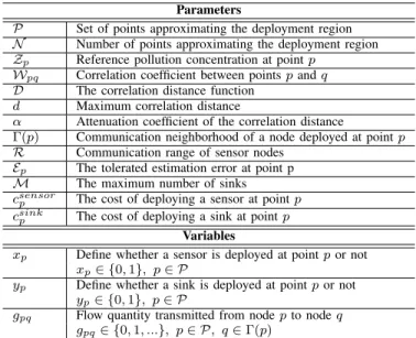
Parameters
P Set of points approximating the deployment region N Number of points approximating the deployment region Zp Reference pollution concentration at point p
Wpq Correlation coefficient between points p and q
D The correlation distance function d Maximum correlation distance
α Attenuation coefficient of the correlation distance
Γ(p) Communication neighborhood of a node deployed at point p R Communication range of sensor nodes
Ep The tolerated estimation error at point p
M The maximum number of sinks csensor
p The cost of deploying a sensor at point p
csinkp The cost of deploying a sink at point p
Variables
xp Define whether a sensor is deployed at point p or not
xp∈ {0, 1}, p ∈ P
yp Define whether a sink is deployed at point p or not
yp∈ {0, 1}, p ∈ P
gpq Flow quantity transmitted from node p to node q
gpq∈ {0, 1, ...}, p ∈ P, q ∈ Γ(p)
TABLE I: Summary of the model notations.
A. Objective function
We consider as input of our model the map of a given urban area that we call the deployment region. We start by discretizing the deployment region in order to get a set of points P approximating the urban area at a high-scale (|P| = N ). Our goal is to be able to determine with a high precision the concentration value at each point p ∈ P . We ensure that for each point p ∈ P , either a sensor is deployed or the pollution concentration can be estimated with a high precision based on the data gathered by the neighboring deployed sensors.
In general case, the set P is thus considered as the set of potential positions of WSN nodes. However, in smart cities applications, some restrictions on node positions may apply because of authorization or practical issues. For instance, in order to alleviate the energy constraints, we may place sensors on only lampposts and traffic lights as experimented in [19]. When this is the case, we do not consider as potential positions the points p ∈ P where sensors cannot be deployed.
We use decision variables xp(respectively yp) to specify if
a sensor (respectively a sink) is deployed at point p or not. Sensors and sinks may have different costs, thus we denote by csensorp (respectively csinkp ) the sensor (respectively the
sink) deployment cost at position p. We summarize in Table I the notations used in the formulations. The deployment cost function to minimize is thus given as follows:
F =X p∈P csensorp ∗ xp+ X p∈P csinkp ∗ yp (2)
B. Air quality coverage
1) Basic formulation: As claimed before, our idea is to base on interpolation methods in order to ensure that the deployed sensors allow to estimate with a high precision the pollution concentrations at locations where no sensor is deployed. This means that we need to have an idea on the dispersion of pollution concentrations in the deployment region in order to be able to formulate the coverage con-straint. More exactly, we need to know the variability of pollution concentrations among the set of points P in order to use the formulation of interpolation methods. Fortunately, using numerical atmospheric dispersion models, we can obtain simulated pollution concentrations that may be considered as reference pollution concentrations [20]. This does not mean that these reference concentrations are real but they reflect the best today’s pollution knowledge.
Let Zp denote the reference concentration value at point
p. Given the set of selected points where sensors will be deployed {p where xp = 1}, we evaluate the estimated
pollution concentrations bZpat points {p where xp= 0} based
on reference values corresponding to the selected points, i.e. based on Zp where p ∈ {p where xp= 1}, as follows:
b Zp= P q∈P−{p}Wpq∗ Zq∗ xq P q∈P−{p}Wpq∗ xq , p ∈ P & xp= 0 X q∈P−{p} Wpq∗ xq> 0, p ∈ P & xp= 0 (3)
The bZp expression is formulated based on formula 1 given
in section III. We have chosen this formula because the weights Wpq are given in a deterministic way, which allows
to integrate them to the ILP deployment model. We ensure that the denominator of bZp is never equal to zero using the
second part of formula 3. The Wpqparameter is the correlation
coefficient between points p and q and is calculated using formula 4 based on the distance between the two points.
D(p, q) is the distance function. α is the attenuation coefficient of the correlation distance, this means that for greater values of α, very low correlation coefficients are assigned to far points. The last parameter of formula 4 is the maximum correlation distance, which defines the range of correlated neighboring points of a given point.
In order to take into account the impact of the urban topography on the dispersion of pollutants, let D be the shortest distance along the roads network. This allows to assign small correlation values to points that are separated by buildings, even if they are close [21].
Wpq= 1 D(p, q)α if q ∈ Disc(p, d) − {p} 0 if q /∈ Disc(p, d) (4)
In order to ensure that the concentration is estimated with high precision at points where no sensor is deployed, we define constraint 5. The Ep parameter corresponds to the estimation
error that is tolerated at point p. The choice of different values of Epin function of p allows to assign low tolerated estimation
errors to locations that are sensitive to air quality such as hospitals, primary schools, etc.
Zbp− Zp ≤ Ep, p ∈ P & xp= 0 (5)
By replacing bZp by its expression given in formula 3, we
obtain the coverage constraints 6 and 7. These two constraints should be linearized in order to get an ILP formulation.
P q∈P−{p}Wpq∗ Zq∗ xq P q∈P−{p}Wpq∗ xq − Zp ≤ Ep, p ∈ P & xp= 0 (6) X q∈P−{p} Wpq∗ xq> 0, p ∈ P & xp= 0 (7)
a) Linearization of constraint 6: The first step is to linearize the fraction part; this allows to get constraint 8. Then, we have to ensure that the constraint is relaxed when xp = 1. To do so, notice that the left member of constraint
8 can be bounded as presented in formula 9. Based on this, we add xp∗Pq∈P−{p}Wpq∗ |Zq− Zp| to the right member
of constraint 8 to relax it when xp = 1. Hence, we obtain
constraint 10. Finally, we have to linearize the absolute-value function. Hence, we get the linear form of constraint 6 in constraints 11 and 12. X q∈P−{p} Wpq∗ xq∗ (Zq− Zp) ≤ Ep∗ X q∈P−{p} Wpq∗ xq, p ∈ P, xp= 0 (8) X q∈P−{p} Wpq∗ xq∗ (Zq− Zp) ≤ X q∈P−{p} Wpq∗ |Zq− Zp| (9) X q∈P−{p} Wpq∗ xq∗ (Zq− Zp) ≤ Ep∗ X q∈P−{p} Wpq∗ xq +xp∗ X q∈P−{p} Wpq∗ |Zq− Zp|, p ∈ P (10) X q∈P−{p} Wpq∗ xq∗ (Zq− Zp) ≤ Ep∗ X q∈P−{p} Wpq∗ xq +xp∗ X q∈P−{p} Wpq∗ |Zq− Zp|, p ∈ P (11) X q∈P−{p} −Wpq∗ xq∗ (Zq− Zp) ≤ Ep∗ X q∈P−{p} Wpq∗ xq +xp∗ X q∈P−{p} Wpq∗ |Zq− Zp|, p ∈ P (12)
b) Linearization of constraint 7: The only thing to do to linearize constraint 7 is to relax the constraint when xp = 1.
This can be obtained by replacing the right member of the constraint by −xp, which allows to get the constraint 13.
X
q∈P−{p}
Wpq∗ xq> −xp, p ∈ P (13)
2) Taking into account sensing drift: Usually, the pollu-tion concentrapollu-tion measured at point q is not equal to the ground truth value Zq and depends on the sensing technology
and the quality of sensors. This involves a certain drift in pollution measurements. The sensing drift is usually given by two parameters aq and bq, which define the measured
concentration that is equal to aq ∗ Zq + bq. By introducing
parameters aq and bq in formula 3, we get in formula 14 the
new definition of the estimated pollution concentration at a given point p depending on the deployed sensors. Using this new definition, we transform the coverage constraints 11 and 12 into constraints 15 and 16, which allows us to include the sensing drift in our coverage model. In this formulation, parameters aq and bq are assumed to be constants. When it is
not the case, stochastic programming should be used instead of integer programming.
b Zp= P q∈P−{p}Wpq∗ (aq∗ Zq+ bq) ∗ xq P q∈P−{p}Wpq∗ xq (14) X q∈P−{p} Wpq∗ xq∗ (aqZq+ bq− Zp) ≤ Ep∗ X q∈P−{p} Wpq∗ xq +xp∗ X q∈P−{p} Wpq∗ |aqZq+ bq− Zp|, p ∈ P (15) X q∈P−{p} −Wpq∗ xq∗ (aqZq+ bq− Zp) ≤ Ep∗ X q∈P−{p} Wpq∗ xq +xp∗ X q∈P−{p} Wpq∗ |aqZq+ bq− Zp|, p ∈ P (16)
3) Taking into account weather conditions: Air pollution dispersion highly depends on weather conditions such as wind and temperature. For instance, reference pollution con-centrations Zp can be totally different if there is a change
in wind direction. In order to cope with that, we consider multiple snapshots of reference concentrations. The resolution of snapshots may be yearly, monthly or daily depending on the needed deployment accuracy and the data availability. Let T be the set of snapshots and Zt
p be the reference pollution
concentration at point p in snapshot t. We propose to ensure that constraints 15 and 16 are verified for each snapshot t ∈ T , hence we get constraints 17 and 18. This allows us to place sensor nodes while taking into account the different weather scenarios corresponding to each pollution snapshot.
X q∈P−{p} Wpq∗ xq∗ (aqZqt+ bq− Zpt) ≤ Ep∗ X q∈P−{p} Wpq∗ xq +xp∗ X q∈P−{p} Wpq∗ |aqZqt+ bq− Zpt|, p ∈ P, t ∈ T (17) X q∈P−{p} −Wpq∗ xq∗ (aqZqt+ bq− Zpt) ≤ Ep∗ X q∈P−{p} Wpq∗ xq +xp∗ X q∈P−{p} Wpq∗ |aqZqt+ bq− Zpt|, p ∈ P, t ∈ T (18) C. Network connectivity
We formulate the connectivity constraint as a network flow problem. We consider the same potential positions set P for sensors and sinks. We first denote by Γ(p), p ∈ P, the set of neighbors of a node deployed at the potential position p. This set can be determined using sophisticated path loss models. It can also be determined using the binary disc model, in which case Γ(p) = {q ∈ P where q ∈ Disc(p, R)} where R is the communication range of sensors. Then, we define the decision variables gpq as the flow quantity transmitted
from a node located at potential position p to another node
located at potential position q. We suppose that each sensor of the resulting WSN generates a flow unit in the network, and verify if these units can be recovered by sinks. The following constraints ensure that the deployed sensors and sinks form a connected wireless sensor network; i.e. each sensor can communicate with at least one sink.
X q∈Γ(p) gpq− X q∈Γ(p) gqp ≥ xp− (N + 1) ∗ yp, p ∈ P (19) X q∈Γ(p) gpq− X q∈Γ(p) gqp ≤ xp, p ∈ P (20) X q∈Γ(p) gpq ≤ N ∗ xp, p ∈ P (21) X p∈P X q∈Γ(p) gpq = X p∈P X q∈Γ(p) gqp (22) X p∈P yp ≤ M (23)
Constraints 19 and 20 are designed to ensure that each deployed sensor, i.e. such that xp = 1, generates a flow unit in
the network. These constraints are equivalent to the following.
X q∈Γ(p) gpq− X q∈Γ(p) gqp = 1 if xp= 1, yp= 0 = 0 if xp= yp= 0 ≤ 0, ≥ −N if xp= 1, yp= 1
The first case corresponds to deployed sensors that should generate, each one of them, a flow unit. The second case, combined with constraint 21, ensures that absent nodes, i.e. xp = yp = 0, do not participate in the communication. The
third case concerns deployed sinks, and ensures that each sink cannot receive more than N units. Constraint 22 means that the overall flow is conservative. The flow sent by deployed sensors has to be received by deployed sinks. Finally, constraint 23 allows to fix the maximum number of sinks M of the resulting network.
D. ILP models
1) Single-level Model: In the first variant of our formula-tion, coverage and connectivity constraints are executed within the same ILP model allowing to get the optimal solution of the deployment problem.
[SLM ]
M inimize (2)
Subject to. (17), (18), (13), (19), (20), (21), (22) and (23)
2) Multilevel Model: In order to allow the execution of the model on large instances, we propose a near-optimal multilevel variant of the ILP model. We first execute MLM-1 to get an optimal coverage solution. Then, we execute MLM-2 that contains the connectivity constraints while fixing to 1 the xp
[M LM − 1]
M inimize (2)
Subject to. (17), (18), (13)
[M LM − 2]
M inimize (2)
Subject to. (19), (20), (21), (22)and (23) V. SIMULATION RESULTS
In this section, we present the simulations that we have performed in order to validate our model and analyze its performances. We first present the data set that we have used and the common simulation parameters. Then, we give a proof-of-concept in order to show how error-bounded deployment is done. Next, we investigate the performance of the two variants of our ILP formulation in terms of execution time and optimal cost. After that, we analyze the network connectivity and pollution coverage results while studying the compromise be-tween the estimation precision and the deployment cost under different configurations of the correlation distance. Finally, we compare the deployment results of our formulation to generic approaches and show the enhancement obtained by our model. A. Dataset
In order to consider the real dispersion of air pollutants in the reference pollution concentrations Zpt, we perform our
simulations on 2 pollution snapshots generated by an enhanced atmospheric dispersion simulator called SIRANE [20]. This simulator is designed for urban areas and takes into account the impact of street canyons on pollution concentrations. The dataset has been provided by Air-Rhone-Alpes, which is an observatory for air pollution monitoring within the Lyon region of France [1].
We depict the 2 reference pollution maps in Figure 1. We focus on nitrogen dioxide (N O2) monitoring since this
pollutant is mainly due to road traffic. We evaluate our ILP model on the La-Part-Dieu district, which is the heart of the Lyon City. Pollution map granularity is around 5 meters and concentrations correspond to the years 2012 and 2013.
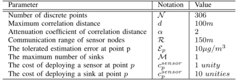
We have implemented the ILP formulations using IBM ILOG CPLEX Optimization Studio and executed them on a PC with Intel Xeon E5649 processor under Linux. Simulation parameters are summarized in Table II. We discretize the de-ployment region which is of around 700m2using a resolution of 50 meters, thus we get 306 discrete points. We consider all these points as potential positions of nodes. We use the same tolerated estimation error Ep = E for all the points p ∈ P.
By default, we use the distance along roads for the evaluation of the correlation coefficients and we suppose that sensing is perfect. In addition, we fix the maximum number of sinks to 1 in order to get mono-sink networks.
Parameter Notation Value Number of discrete points N 306 Maximum correlation distance d 100m Attenuation coefficient of correlation distance α 2 Communication range of sensor nodes R 150m The tolerated estimation error at point p Ep 10µg/m3
The maximum number of sinks M 1 The cost of deploying a sensor at point p csensor
p 1 unity
The cost of deploying a sink at point p csensorp 10 unities
TABLE II: Default values of simulation parameters.
B. Validation by experiments
In order to validate our formulation of error-bounded WSN deployment, we run the single-level model using the 2 ref-erence pollution maps while considering 3 values for the tolerated estimation error: 2, 5 and 8 µg/m3. We depict
in table III the resulting optimal cost corresponding to the snapshot of 2012 alone, the snapshot of 2013 alone and the two snapshots together (using formulations given in section IV-B3). We notice that snapshot 2012 needs more sensors than snapshot 2013. This is because the range of pollution concentrations is larger in snapshot 2012 as shown in figure 1, which involves higher pollution variability and thus more interpolation errors. In addition, when trying to satisfy both of the two snapshots, we place at least the sensors that are required by snapshot 2012 since this snapshot is more complicated than the other one.
Tolerated estimation error 2µg/m3 5µg/m3 8µg/m3 Snapshot 2012 alone 221 146 105 Snapshot 2013 alone 171 67 48 Snapshots 2012 and 2013 together 237 148 105
TABLE III: Deployment cost (monetary units) depending on snapshots and the tolerated estimation error.
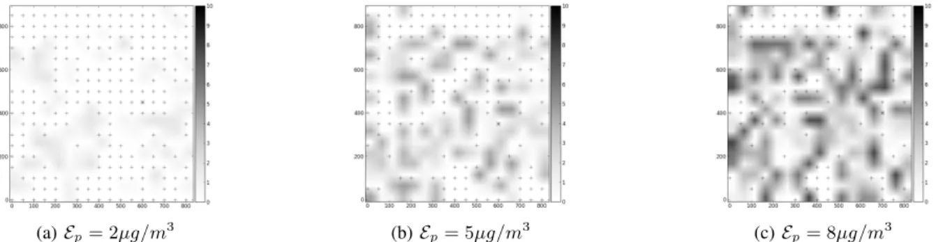
We now depict in Figure 2 the obtained positions of sensors and sinks when using only snapshot 2012. We evaluate at each point of the map the estimated concentration and then we cal-culate the resulting estimation error, i.e. the difference between the reference concentrations and the estimated concentrations. The obtained errors are also depicted in Figure 2.
We notice that more sensors are used when the tolerated estimation error decreases. This is expected since better de-ployment precision needs more sensor nodes. In addition, Figure 2 shows that the maximum error value is bounded by the tolerated estimation error, which fits with our coverage formulation. Moreover, the obtained nodes form a connected network as formulated in our connectivity constraint. In the next simulation cases, we execute the model only on the snapshot of year 2012.
C. Performance evaluation
In this section, we compare the two variants of our ILP model in terms of execution time and objective function. We depict in Figure 3 the deployment cost depending on the tolerated estimation error while executing the single-level
(a) NO2 concentrations (µg/m3) of 2012 (b) NO2 concentrations (µg/m3) of 2013
Fig. 1: Reference NO2 concentrations in Lyon La-Part-Dieu district, average over years 2012 and 2013 (Ref:Air-Rhone-Alpes).
(a) Ep= 2µg/m3 (b) Ep= 5µg/m3 (c) Ep= 8µg/m3
Fig. 2: Deployments with increasing estimation errors (µg/m3) for snapshot 2012. Sensors (respectively sinks) are depicted using "plus signs" (respectively stars).
model, the multilevel model and the coverage formulation alone.
Fig. 3: Deployment cost vs. tolerated estimation error.
We notice that the deployment cost given by the two variants is greater than the coverage cost. This is mainly due to the cost of the sink that ensures the connectivity of the network. We also notice that the near-optimal multilevel model gives the same values as the optimal single-level model when the tolerated estimation error is less than 7µg/m3. This is explained by the fact that for small values of the tolerated estimation error, the network that results from the first stage of the multilevel model, i.e. the coverage formulation, is usually dense and needs no more relay nodes to be connected. However, we notice in Table IV that the execution time is significantly enhanced when using the multilevel model. Indeed, the enhancement factor exceeds 100 in some cases.
The difference in execution time between the two models should be larger when applied on large-scale areas. As a conclusion, the multilevel model allows to get good solutions, and even optimal solutions for high-precision deployments, in a reasonable time.
Tolerated estimation error Single-level Model Multilevel Model 3 µg/m3 1.59 s 0.16 s
6 µg/m3 25.23 s 0.19 s
9 µg/m3 32.45 s 0.27 s 12 µg/m3 6.74 102 s 1.65 s
TABLE IV: Execution time vs. tolerated estimation error.
D. Evaluation of the network connectivity
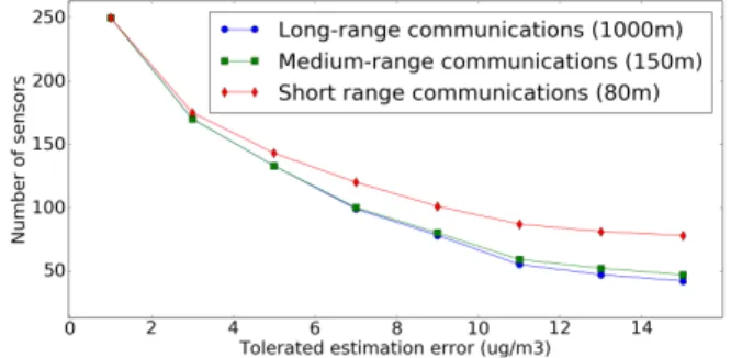
In this simulation case, we analyze the deployment cost that is due to the connectivity constraint, which involves the deployment of sink and relay nodes. We consider 3 possible values of the communication range of sensor nodes: 80m for short range communications like ZigBee, 150m for medium range communications like WiFi and 1000m for long-range communications. We evaluate the number of nodes depending on the tolerated estimation error and depict the results in Fig. 4. Obviously, the longer the communication range, the less the number of sensors is. However, the tolerated estimation error has a considerable impact on the connectivity of the network. On the one hand, the medium and long range communications
involve nearly the same number of nodes. For instance, when estimation errors are less than 10µg/m3, the medium range
communications need at most only two more nodes than the high range communications. This is explained by the fact that small tolerated errors imply a very high density of the network so that sensors are placed almost in all positions. On the other hand, short range communications are very costly and need almost 70% more nodes than the long range communications when the estimation errors reach 15µg/m3. This is because the distance between sensor nodes that are responsible for coverage is very important when high estimation errors are tolerated, which causes the need of too much relay nodes if the communication range is very short.
Fig. 4: Optimal number of sensors depending on the commu-nication range.
E. Evaluation of the coverage results
In this simulation scenario, we study the dependency be-tween the deployment precision and the needed number of sen-sors under different configurations of the correlation distance. Since we are studying the cost of the monitoring precision, we execute only the coverage constraint. We depict in Figure 5 the optimal deployment cost depending on the tolerated es-timation error while considering two different functions of the correlation distance: the Euclidean distance and the distance along roads. We notice in the two curves that less sensors are needed when the tolerated estimation error decreases. This is because less tolerated estimation error involves high-precision deployment and thus more nodes. In addition, the Euclidean distance gives less number of sensors, which is explained by the fact that the distance along roads is more realistic and hence involves more nodes to better estimate pollution concentrations.
Fig. 5: Optimal coverage cost vs. tolerated estimation error.
We now investigate the impact of the correlation distance on the number of sensors that are needed to cover a point where no sensor in deployed. We consider different configurations of the maximum correlation distance d and the attenuation coefficient of the correlation distance α. We depict in Figure 6 the average number of sensors that are deployed within the maximum correlation distance d of each point where no sensor is deployed. We notice that less sensors are used when considering greater values of the attenuation coefficient α and less values of the maximum correlation distance d. To explain this, we recall that smaller values of the d parameter allow to consider less points in the interpolation formula, and higher values of the α parameter allow to assign smaller values of correlation coefficients to the far sensors. This means that with smaller values of d and higher values of α, the interpolation is done with less sensors, which fits with the results depicted in Figure 6.
(a) Impact of the maximum correlation distance
(b) Impact of the attenuation coefficient of correlation distance
Fig. 6: Impact of correlation distance parameters on the mean number of neighbors per point.
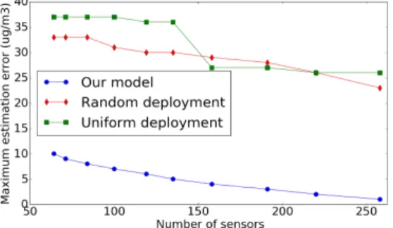
F. A comparison with generic deployment approaches To the best of our knowledge, existing deployment models assume that a sensor has a given detection range, which is not the case of pollution sensors. Instead of that, we constraint the deployment by the error of estimated maps. We believe that the comparison with detection range based solutions would not be convincing since the two approaches are based on different coverage definitions. However, our model can be compared to generic deployment methods based on our coverage definition. Hence, we propose a comparison with random and uniform approaches.
In order to show the enhancement factor of our formulation, we evaluate the maximum estimation error of the estimated pollution concentrations while varying the number of sensors
and the deployment approach. Results are depicted in Fig. 7. We consider random and uniform deployment in addition to our coverage formulation. For random deployment, we depict the average of 100 simulations for each value of the X-axis. The obtained results show that our model is at least 3 times better than the other approaches, which gave nearly the same results. Moreover, the enhancement factor increases with the number of sensors. For instance, when using 258 nodes, the maximum error given by our model is equal to 1µg/m3 whereas uniform and random approaches gave, respectively, 26µg/m3 and 23µg/m3.
Fig. 7: Comparison results
VI. CONCLUSION AND FUTURE WORK
In this paper, we tackled the optimization problem of sensor deployment and proposed integer programming models computing a cost-optimal network topology while ensuring the mapping of air quality with bounded error. Our main contribution is to constraint the deployment of sensors by the quality of the pollution estimation that can be interpolated between the sensors. We applied our model on a dataset of the Lyon City, and have shown how error-bounded deployment is done. We also investigated the performance of our ILP formulation and studied the trade-off between the deployment precision and the deployment cost.
As a future work, we plan to consider the impact of the different urban parameters such as the structure of streets on the deployment results. Moreover, we are also working on the design of specific heuristics to solve the addressed problem faster.
ACKNOWLEDGMENT
This work has been supported by the "LABEX IMU" (ANR-10-LABX-0088) and the "Programme Avenir Lyon Saint-Etienne" of Université de Lyon, within the program "Investissements d’Avenir" (ANR-11-IDEX-0007) operated by the French National Research Agency (ANR).
REFERENCES
[1] Air Rhône-Alpes, “The air quality monitoring organization of the lyon agglomeration,” http://www.air-rhonealpes.fr [2016-01-27].
[2] A. Kumar, H. Kim, and G. P. Hancke, “Environmental monitoring systems: a review,” Sensors Journal, IEEE, vol. 13, no. 4, pp. 1329– 1339, 2013.
[3] J. Yick, B. Mukherjee, and D. Ghosal, “Wireless sensor network survey,” Computer networks, vol. 52, no. 12, pp. 2292–2330, 2008.
[4] M. Mead, O. Popoola, G. Stewart, P. Landshoff, M. Calleja, M. Hayes, J. Baldovi, M. McLeod, T. Hodgson, J. Dicks et al., “The use of electrochemical sensors for monitoring urban air quality in low-cost, high-density networks,” Atmospheric Environment, vol. 70, pp. 186–203, 2013.
[5] D. Hasenfratz, O. Saukh, C. Walser, C. Hueglin, M. Fierz, and L. Thiele, “Pushing the spatio-temporal resolution limit of urban air pollution maps,” in Pervasive Computing and Communications (PerCom), 2014 IEEE International Conference on. IEEE, 2014, pp. 69–77.
[6] A. Marjovi, A. Arfire, and A. Martinoli, “High resolution air pollu-tion maps in urban environments using mobile sensor networks,” in Distributed Computing in Sensor Systems (DCOSS), 2015 International Conference on. IEEE, 2015, pp. 11–20.
[7] S. Devarakonda, P. Sevusu, H. Liu, R. Liu, L. Iftode, and B. Nath, “Real-time air quality monitoring through mobile sensing in metropolitan areas,” in Proceedings of the 2nd ACM SIGKDD International Workshop on Urban Computing. ACM, 2013, p. 15.
[8] C. Zhu, C. Zheng, L. Shu, and G. Han, “A survey on coverage and connectivity issues in wireless sensor networks,” Journal of Network and Computer Applications, vol. 35, no. 2, pp. 619–632, 2012. [9] K. Chakrabarty, S. S. Iyengar, H. Qi, and E. Cho, “Grid coverage
for surveillance and target location in distributed sensor networks,” Computers, IEEE Transactions on, vol. 51, no. 12, pp. 1448–1453, 2002. [10] B. Liu, O. Dousse, P. Nain, and D. Towsley, “Dynamic coverage of mobile sensor networks,” Parallel and Distributed Systems, IEEE Transactions on, vol. 24, no. 2, pp. 301–311, 2013.
[11] ˙I. K. Altınel, N. Aras, E. Güney, and C. Ersoy, “Binary integer programming formulation and heuristics for differentiated coverage in heterogeneous sensor networks,” Computer Networks, vol. 52, no. 12, pp. 2419–2431, 2008.
[12] M. E. Keskin, ˙I. K. Altınel, N. Aras, and C. Ersoy, “Wireless sensor network lifetime maximization by optimal sensor deployment, activity scheduling, data routing and sink mobility,” Ad Hoc Networks, vol. 17, pp. 18–36, 2014.
[13] M. Rebai, H. Snoussi, F. Hnaien, L. Khoukhi et al., “Sensor deployment optimization methods to achieve both coverage and connectivity in wireless sensor networks,” Computers & Operations Research, vol. 59, pp. 11–21, 2015.
[14] S. Sengupta, S. Das, M. Nasir, and B. K. Panigrahi, “Multi-objective node deployment in wsns: In search of an optimal trade-off among coverage, lifetime, energy consumption, and connectivity,” Engineering Applications of Artificial Intelligence, vol. 26, no. 1, pp. 405–416, 2013. [15] J. D. Marshall, E. Nethery, and M. Brauer, “Within-urban variability in ambient air pollution: comparison of estimation methods,” Atmospheric Environment, vol. 42, no. 6, pp. 1359–1369, 2008.
[16] M. Jerrett, A. Arain, P. Kanaroglou, B. Beckerman, D. Potoglou, T. Sahsuvaroglu, J. Morrison, and C. Giovis, “A review and evaluation of intraurban air pollution exposure models,” Journal of Exposure Science and Environmental Epidemiology, vol. 15, no. 2, pp. 185–204, 2005. [17] D. W. Wong, L. Yuan, and S. A. Perlin, “Comparison of spatial
interpolation methods for the estimation of air quality data,” Journal of Exposure Science and Environmental Epidemiology, vol. 14, no. 5, pp. 404–415, 2004.
[18] G. Hoek, R. Beelen, K. De Hoogh, D. Vienneau, J. Gulliver, P. Fischer, and D. Briggs, “A review of land-use regression models to assess spatial variation of outdoor air pollution,” Atmospheric environment, vol. 42, no. 33, pp. 7561–7578, 2008.
[19] V. Gallart, S. Felici-Castell, M. Delamo, A. Foster, and J. J. Perez, “Evaluation of a real, low cost, urban wsn deployment for accurate en-vironmental monitoring,” in Mobile Adhoc and Sensor Systems (MASS), 2011 IEEE 8th International Conference on. IEEE, 2011, pp. 634–639. [20] L. Soulhac, P. Salizzoni, P. Mejean, D. Didier, and I. Rios, “The model sirane for atmospheric urban pollutant dispersion; part II, validation of the model on a real case study,” Atmospheric Environment, vol. 49, pp. 320–337, 2012.
[21] A. Tilloy, V. Mallet, D. Poulet, C. Pesin, and F. Brocheton, “Blue-based no2 data assimilation at urban scale,” Journal of Geophysical Research: Atmospheres, vol. 118, no. 4, pp. 2031–2040, 2013.