Comprehensive Classification of Retinal Bipolar
Neurons by Single-Cell Transcriptomics
The MIT Faculty has made this article openly available.
Please share
how this access benefits you. Your story matters.
Citation
Shekhar, Karthik et al. “Comprehensive Classification of Retinal
Bipolar Neurons by Single-Cell Transcriptomics.” Cell 166, 5
(August 2016): 1308–1323 © 2016 Elsevier Inc
As Published
http://dx.doi.org/10.1016/J.CELL.2016.07.054
Publisher
Elsevier
Version
Author's final manuscript
Citable link
http://hdl.handle.net/1721.1/116759
Terms of Use
Creative Commons Attribution-Noncommercial-Share Alike
COMPREHENSIVE CLASSIFICATION OF RETINAL BIPOLAR
NEURONS BY SINGLE-CELL TRANSCRIPTOMICS
Karthik Shekhar1,*, Sylvain W. Lapan2,*, Irene E. Whitney4,*, Nicholas M. Tran4, Evan Z. Macosko2,5,6, Monika Kowalczyk1, Xian Adiconis1,5, Joshua Z. Levin1,5, James
Nemesh2,5,6, Melissa Goldman2,5, Steven A. McCarroll2,5,6, Constance L. Cepko2,3,7,#, Aviv Regev1,7,8,#, and Joshua R. Sanes4,†
1Broad Institute of Harvard and MIT, Cambridge, MA 02142, USA
2Department of Genetics, Harvard Medical School, Boston, MA 02115, USA 3Department of Ophthalmology, Harvard Medical School, Boston, MA 02115, USA
4Center for Brain Science and Department of Molecular and Cellular Biology, Harvard University,
Cambridge, MA 02130, USA
5Stanley Center for Psychiatric Research, Broad Institute of Harvard and MIT, Cambridge, MA
02142, USA
6Program in Medical and Population Genetics, Broad Institute of Harvard and MIT, Cambridge,
MA 02142, USA
7Howard Hughes Medical Institute, Chevy Chase, MD 20815, USA
8Department of Biology and Koch Institute, MIT, Cambridge, MA 02139, USA
SUMMARY
Patterns of gene expression can be used to characterize and classify neuronal types. It is challenging, however, to generate taxonomies that fulfill the essential criteria of being
comprehensive, harmonizing with conventional classification schemes, and lacking superfluous subdivisions of genuine types. To address these challenges, we used massively parallel single-cell RNA profiling and optimized computational methods on a heterogeneous class of neurons, mouse retinal bipolar cells (BCs). From a population of ~25,000 BCs we derived a molecular
†Lead Contact: [email protected].
*Co-first authors #Co-corresponding authors [email protected] [email protected] AUTHOR CONTRIBUTIONS
Conceptualization, K.S., S.W.L., I.E.W, C.L.C., A.R., J.R.S.; Software, K.S., J.N; Validation and Formal Analysis, K.S., S.W.L., I.E.W., N.T.; Drop-seq experiments, E.Z.M, M.G., S.A.M.; Smart-seq2 experiments, X.A.; Resources, M.K., J.Z.L., S.A.M.; Data Curation, K.S., E.Z.M., Writing – Original Draft, K.S., S.W.L., I.E.W, A.R., J.R.S; Writing – Review & Editing, N.M.T., E.Z.M, S.A.M, C.L.C; Visualization, K.S., S.W.L., I.E.W, N.T;
Publisher's Disclaimer: This is a PDF file of an unedited manuscript that has been accepted for publication. As a service to our customers we are providing this early version of the manuscript. The manuscript will undergo copyediting, typesetting, and review of
HHS Public Access
Author manuscript
Cell
. Author manuscript; available in PMC 2017 August 25.Published in final edited form as:
Cell. 2016 August 25; 166(5): 1308–1323.e30. doi:10.1016/j.cell.2016.07.054.
A
uthor Man
uscr
ipt
A
uthor Man
uscr
ipt
A
uthor Man
uscr
ipt
A
uthor Man
uscr
ipt
classification that identified 15 types including all types observed previously, and two novel types, one of which has a non-canonical morphology and position. We validated the classification scheme and identified dozens of novel markers using methods that match molecular expression to cell morphology. This work provides a systematic methodology for achieving comprehensive molecular classification of neurons, identifies novel neuronal types, and uncovers transcriptional differences that distinguish types within a class.
eTOC
Single-cell transcriptome sequencing of retinal bipolar cells reveals known and new types including one with a non-canonical morphology.
INTRODUCTION
Investigations into brain development, function, and disease depend upon accurate
identification and categorization of cell types. Assignment of roles, genes, or pathologies to specific types allows fundamental processes to be understood with greater precision than when assigned to brain regions or broad classes of cells. Moreover, molecular identifiers of specific types enable comparison of results obtained at different times, in different
laboratories, or following experimental perturbations. In model organisms, they enable genetic access, allowing neurons to be marked and manipulated. Accordingly, numerous methods have been developed to classify neurons (Seung and Sumbul, 2014).
Despite methodological advances, the enterprise of cell type categorization remains
challenging for both technical and conceptual reasons. Conceptually, the very definition of a “cell type” is contentious. Existing taxonomies represent neurons as a hierarchy of types whose distinctions reflect criteria such as morphology, physiology, and gene expression (Sanes and Masland, 2015). While distinctions at the upper levels of this hierarchy are easily agreed upon (e.g. sensory vs. motor neurons), finer divisions are less obvious. It is also
A
uthor Man
uscr
ipt
A
uthor Man
uscr
ipt
A
uthor Man
uscr
ipt
A
uthor Man
uscr
ipt
unclear whether distinctions based on morphological, molecular, and physiological properties agree with each other. Finally, some distinctions are difficult to quantify. Indeed, few diverse neuronal classes have been comprehensively partitioned into types.
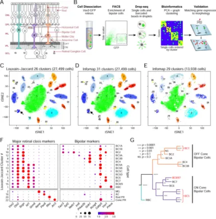
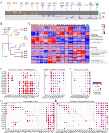
A taxonomy based on molecular features is a potential solution to these problems. Several recent studies have used single-cell RNA sequencing (scRNA-seq) to group cells into types based on gene expression signatures (Darmanis et al., 2015; Macosko et al., 2015; Pollen et al., 2014; Tasic et al., 2016; Usoskin et al., 2015; Zeisel et al., 2015). However, these studies have not been able to determine whether the groups represent distinct types, or whether all types in the population are represented. Among many obstacles, two stand out. First, the number of cells profiled to date, typically ranging from a hundred to a few thousand, is likely too few for complete sampling and categorization. Second, satisfactory classification requires that molecular criteria be validated against an orthogonal criterion of cell type. To address these challenges, we set out to generate a comprehensive, validated classification scheme for a diverse class of interneurons, the bipolar cells (BCs) of the mouse retina. BCs receive synaptic input from rod and cone photoreceptors, process it in diverse ways, and transmit it to retinal ganglion cells (RGCs), which in turn send axons to the rest of the brain (Figure 1A). BCs are divided into rod and cone types, based on the photoreceptors from which they receive their predominant synaptic input. They are also divisible into ON and OFF types based on whether they are excited (depolarized) by increases or decreases in illumination level. BCs have been divided into 9–12 types, initially by morphological features, which were later related to physiological and, in some cases, molecular properties (Euler et al., 2014; Helmstaedter et al., 2013; Wassle et al., 2009). This prior knowledge is useful for evaluating computational methods, and for validating novel markers or types. To comprehensively study BCs in a cost-effective manner we used Drop-seq, a
high-throughput scRNA-seq method that utilizes droplet microfluidics (Macosko et al., 2015). We profiled ~28,000 cells from a transgenic mouse line that marks BCs. This is 10–30 fold more cells than analyzed in recent studies but at far lower sequencing coverage per cell. We applied scalable computational methods to identify cell types. To assess the tradeoff between cell number and sequencing depth for resolving cell types, we performed parallel
experiments using conventional scRNA-seq. To relate clusters defined by unsupervised computational analyses to known BC types, we used previously described type-specific markers, 10 transgenic lines, and a validation method that combines fluorescent in situ hybridization (FISH) with sparse viral labeling. Together, these approaches allowed us to match molecularly defined with morphologically defined BC types (Figure 1B).
Our work addresses three key questions, two of which are technological: (1) how can one best use scRNA-seq to classify neuronal types, and (2) can genes relevant for functional differences among types be identified from an unbiased inquiry? In answering these questions, we present a framework that can be used for similar analyses of other
heterogeneous cell populations. The third question is neurobiological: what is the full cohort of BC types? In answering this question, we identified 15 transcriptionally distinct BC types, including all types identified previously (Euler et al., 2014), as well as two that had not previously been described. We also identified molecular markers for each BC type. The vast
A
uthor Man
uscr
ipt
A
uthor Man
uscr
ipt
A
uthor Man
uscr
ipt
A
uthor Man
uscr
ipt
majority of BCs displayed transcriptional profiles of a single type, with scant evidence for intermediate types or continua of transcriptional identities.
RESULTS
Drop-seq of single retinal bipolar neurons
BCs comprise ~7% of all retinal cells in mice (Jeon et al., 1998). To obtain an enriched population, we used a transgenic line that expresses GFP in all BCs and Müller glia (Vsx2-GFP) (Rowan and Cepko, 2004). We collected GFP-positive cells by fluorescence activated cell sorting (Figure 1B), and prepared scRNA-seq libraries using Drop-seq, wherein single cells are paired in droplets with single microparticle beads coated with oligonucleotides for reverse transcription (Macosko et al., 2015). These oligonucleotides contain a bead-specific barcode (“cell barcode”) uniquely identifying each bead (cell), and a unique molecular identifier (UMI) that allows “amplification duplicates” to be recognized and discarded. Thousands of beads can be processed in a single reaction, dramatically reducing labor and reagent costs.
We obtained data from 45,000 cells, sequenced to a median depth of 8,200 mapped reads per cell (Figure S1A–H, Table S1), and derived a digital expression matrix of 13,166
appreciably expressed genes across 27,499 cells after aligning reads, demultiplexing and counting UMIs. After correcting for batch effects, we applied principal component (PC) analysis, retained the 37 statistically significant PC scores (p<10−3, Figure S1I, J), and visualized the cells in two dimensions using t-distributed stochastic neighborhood embedding (t-SNE; Figure 1C–E, S1K; see Methods and Resources for details). Unbiased graph clustering identifies 26 putative cell type clusters
We tested six unsupervised computational approaches for clustering cells by their transcriptional profiles, without reference to prior knowledge of BC types or markers (Methods and Resources, Figure S2). Two graph clustering algorithms, Louvain-Jaccard (Blondel et al., 2008; Levine et al., 2015) and Infomap (Rosvall and Bergstrom, 2008), exhibited superior performance as judged by a post hoc comparison of predicted clusters to known BC types, their ability to resolve clusters when applied to subsets of the data, and their computational scalability (Figure 1C, D; Methods and Resources). Infomap nominated a larger number of clusters than Louvain-Jaccard (Figure S2A, F), but most differences disappeared upon merging transcriptionally proximal clusters (Figure 1C, D). We focused subsequent validation efforts on the output of Louvain-Jaccard, which produced the fewest spurious clusters prior to merging. We obtained the same clusters when the analysis was repeated using only 50% of the cells in the dataset, but some clusters were merged when only 18% of cells were analysed (Figure 1E, S2K, L, N), suggesting that large numbers of cells are important for resolving transcriptionally similar types.
Fourteen BC clusters, seven align with known types
Fourteen of the 26 clusters generated by Louvain-Jaccard were identifiable as BCs by expression of the pan-BC markers Vsx2 and Otx2 (Baas et al., 2000; Burmeister et al., 1996), and absence of markers of other retinal classes (clusters 1 and 3–15; Figure 1C, F).
A
uthor Man
uscr
ipt
A
uthor Man
uscr
ipt
A
uthor Man
uscr
ipt
A
uthor Man
uscr
ipt
These clusters comprised 84% of all cells analyzed vs. 7% in the whole retina, indicating that FACS resulted in a 12-fold enrichment of BCs. Müller glia (cluster 2), which are also labeled in the Vsx2-GFP line, comprised 10.5% of cells. The remaining 11 clusters,
comprising <4% of the dataset, included rods, cones, amacrine cells and cell doublets (Table S2). It is a strength of scRNA-seq methods that undesired types can be identified and excluded from further analysis rather than contaminating the transcriptomes of the relevant types.
We assigned the 14 BC clusters to types by inspecting the expression of known markers (Table S2). Clusters could be divided into rod and cone BCs based on the presence or absence of RBC markers (e.g., Prkca; cluster 1) or the broad cone BC marker, Scgn (3–15; Figure 1F) (Kim et al., 2008b; Puthussery et al., 2010). The cone BC clusters could be further divided into ON (3–6, 13, 15) and OFF (7–10, 12, 14) BC types based on the ON bipolar markers Isl1 and/or Grm6 (Elshatory et al., 2007; Ueda et al., 1997). Additional known markers allowed for the 1:1 assignment of six clusters (4, 5, 8, 10, 12, and 14) to six matching cone BC types (BC7, 6, 3B, 2, 3A and 4, respectively) (Figure 1F, Table S2). Figure 1G shows relationships among putative BC types, determined by hierarchical clustering (Methods and Resources). These types were consistently reproduced in a reanalysis of ~5,500 BCs from our recent whole retina Drop-seq study (Macosko et al., 2015) (Figure S3A–F).
Seven BC clusters (3, 6, 7, 9, 11, 13 and 15) could not be unequivocally assigned to known types. We tentatively labeled them based on marker expression (Figure 1F) and relationships to known types (Figure 1G). We investigate these “mystery” clusters below.
Validated molecular markers for six BC types
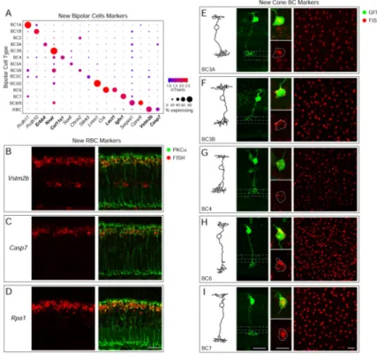
To identify markers for BC types, we devised a binomial test to find genes differentially expressed between clusters (Figures 2A, S3G, Table S3). To relate markers to cellular morphology, we developed a method for sparse labeling of BCs using a lentivirus with a Vsx2 enhancer to express GFP in BCs, and combined this with fluorescent in situ
hybridization (FISH) (Table S4, Methods and Resources). In some cases we also combined FISH with an antibody or a transgenic reporter mouse line.
More than 100 genes were enriched in the RBC cluster (FDR < 0.01) (Table S3), including all previously reported RBC markers and numerous additional candidates. We tested 25 candidate genes and validated expression of all 25 using FISH in combination with a RBC-specific antibody, PKCα (Figures 2B–D and S4A). We also validated expression of several low abundance genes, which were RBC-specific but detected in <30% of the cells in cluster 1 (Figure S4A–C). Thus, the ability to sample a large number of cells across multiple types enables identification of markers across a wide range of expression levels.
We next validated new markers for BC types 3A, 3B, 4, 6 and 7 (Figure 2A, Table S3). The morphology of FISH-positive cells revealed by sparse lentiviral labeling was matched to reconstructions from electron microscopy (Helmstaedter et al., 2013) (Figure 2E–I, leftmost panels). Erbb4, Nnat, Col11a1, Lect1, and Igfn1 labeled cells that corresponded in arbor shape and lamination with BC3A, 3B, 4, 6, and 7 respectively (Figure 2E–I, middle panels).
A
uthor Man
uscr
ipt
A
uthor Man
uscr
ipt
A
uthor Man
uscr
ipt
A
uthor Man
uscr
ipt
We further validated markers for all five types by combinatorial labeling with known markers and use of transgenic lines (Figure S5A–E). Many BC2 markers have been identified previously (Chow et al., 2004; Fox and Sanes, 2007; Haverkamp et al., 2003), all of which were enriched in cluster 10 (Figure S5F). We also devised a FISH protocol to label retinal whole mounts and confirmed that patterns of labeled somata across the whole retina were consistent with authentic neuronal types (Figure 2E–I, rightmost panels).
Together, these results validate markers for 7 BC types. We next turned to the remaining 7 BC clusters, which were less readily assigned to known types.
A BC1 variant with amacrine-like morphology
Clusters 7 and 9 both expressed BC1 markers (Tacr3+Rcvrn−Syt2−). This was unexpected, as previous studies had indicated BC1 to be a single population (Helmstaedter et al., 2013; Wassle et al., 2009). Although these clusters (BC1A and BC1B) were each other’s closest relatives (Figure 1G), 139 genes were >2 fold differentially expressed between them (FDR < 0.01), suggesting that they represented distinct cell types (see Figure 3A for examples). To explore whether BC1A and 1B were morphologically distinct, we used the MitoP transgenic line in which CFP is expressed in BC1s and an amacrine cell (AC) type called nGnG (Kay et al., 2011; Schubert et al., 2008). BC1A markers labeled cells with bipolar morphology. Surprisingly, BC1B markers labeled cells that were unipolar, lacking a dendrite extending to the outer plexiform layer (OPL), where BCs are innervated by photoreceptors (Figures 3B, S6A–F). Moreover, BC1A somata were intermingled with other BCs nearer the OPL border, whereas BC1B somata were located closer to the IPL, amongst AC somata. Nonetheless, BC1B cells, expressed pan-BC markers but neither pan-AC markers nor the nGnG AC marker Ppp1r17 (Figures 1F, 3A, C).
We confirmed the unusual morphology of BC1B cells using the lentiviral method and a Fezf1-cre knock-in mouse line (Figures 3D–F, S6G). Moreover, (Della Santina et al., 2016) recently observed cells that likely correspond to BC1B in another transgenic line, and confirmed that their synaptic ultrastructure is characteristic of BC axon terminals. As BC1B cells have BC-AC hybrid properties, we asked whether their developmental origins
resembled those of BCs or ACs. We stained MitoP retinas at multiple ages with an antibody against Lhx3, which is expressed by BC1B but not BC1A cells (Figure 3A, S6L). We observed two sets of CFP+ Lhx3+ cells, those with a bipolar morphology in the outer part of the INL, where conventional BCs reside, and those with a unipolar morphology closer to where ACs are located. The percentage of CFP+ Lhx3+ cells with a unipolar rather than bipolar morphology progressively increased from 3% at P6 to over 80% by P17 (Figure 3G). BC1B cells with short, seemingly retracting dendrites were observed at an intermediate position at P6–8. Thus, both BC1 types originate with a bipolar morphology, but BC1B cells lose their apical process and translocate to the amacrine layer (Figures 3H, I, S6H–K). Four distinct BC5 types
To date, molecular studies have revealed only a single BC5 type in mice (Wassle et al., 2009), but morphological and physiological analyses have shown the existence of two
BC5-A
uthor Man
uscr
ipt
A
uthor Man
uscr
ipt
A
uthor Man
uscr
ipt
A
uthor Man
uscr
ipt
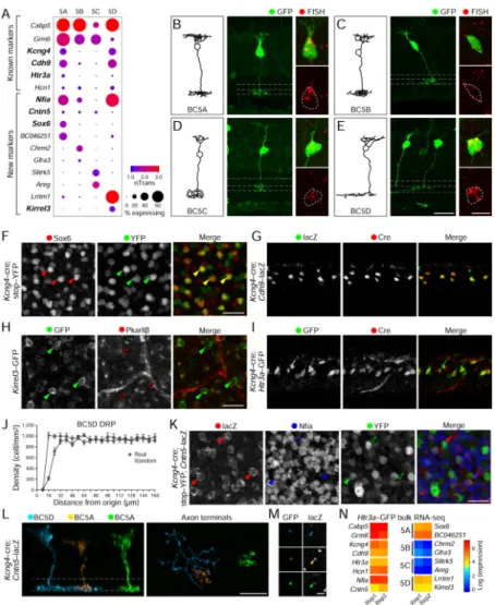
proximity to BC5 (Hellmer et al., 2016; Helmstaedter et al., 2013). Our unsupervised analysis identified four BC5 clusters (Figure 1G), which we termed BC5A–D, as they expressed known BC5 makers (Figure 4A) (Duan et al., 2014; Haverkamp et al., 2003; Hellmer et al., 2016; Wassle et al., 2009).
Using the lentivirus/FISH method, we found that BC5A–D axons all arborized in the sublamina characteristic of canonical BC5s, but displayed morphological distinctions (Figure 4B–E). BC5A (Sox6+) and BC5B (Chrm2+), had narrow monostratified axonal arbors, but only the former extended large dendritic stalks to the OPL, a feature of the ultrastructurally defined BC5A. BC5C (Slitrk5+) cells had bistratified axons. BC5D (Lrrtm1+) cells had wide, thin arbors reminiscent of XBCs (Helmstaedter et al., 2013). We next analyzed five mouse lines that report on the expression of genes enriched in specific BC5 types (Kcng4-cre, Kirrel3-GFP, Cntn5-tau-lacZ, Cdh9-lacZ, and Htr3a-GFP; Figure 4A). In each case results validated patterns predicted from Drop-seq. (Figure 4F–M). Moreover, bulk RNA-seq of GFP+ cells from the Htr3a-GFP line confirmed the expression of markers from the BC5A and BC5D but not BC5B/BC5C clusters (Figure 4N, Methods and Resources). Together, these results provide a definitive division of BC5 into four groups, and a set of transgenic lines with which they can be marked.
BC8 and 9 identified through an alternative unsupervised method
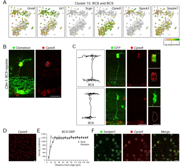
ON BC8 and 9 were the only known BC types that remained unaccounted for, and no endogenous markers of either type have been identified. Cluster 15 expressed markers of ON cone BCs, but no known markers of specific BC types (Figure 1F, 5A). We asked whether Cluster 15 contained BC8 and or BC9. Cluster 15 was unique in comprising two visibly separate lobes on the t-SNE map, suggesting the possibility of sub-populations (Figures 1C, 5A). These clusters were distinguished by applying the Infomap algorithm (Figure 1D), with 71 DE genes (>2-fold expression difference FDR < 0.01). The most specific marker for Cluster 15, Cpne9, was expressed exclusively in one of the two putative sub-populations (Figure 5A). Neither of the general ON BC markers, Grm6 or Isl1 exhibited this bias. These observations suggested that cluster 15 contains both BC8 and BC9 cells, with Cpne9 marking one type. (Figures 2A, 5A). To test this idea, we used the Thy1-Clomeleon-1 (Clm-1) line, previously described to label BC9 cells (Breuninger et al., 2011; Haverkamp et al., 2005). BCs that expressed clomeleon (a YFP/CFP fusion) were Cpne9+, indicating this to be a marker for BC9 (Figure 5B). We also identified both Cpne9+ and Cpne9− cells with BC8/9-like morphology using the FISH/lentiviral method (Figure 5C); likewise, two-color FISH identified two populations of Seripini1+ cells (a marker of both subclusters), some Cpne9+ (BC9) and others Cpne9− (BC8) (Figure 5F). Cpne9+ somas in retinal whole mount exhibit uniform spacing (Figure 5D, E), consistent with this being a single cell type. We conclude that Serpini1+ Cpne9− and Serpini1+ Cpne9+ BCs correspond to BC8 and 9, respectively.
Taken together, our histological validation of a computationally derived molecular taxonomy unifies molecular and morphological signatures of BCs (Figure 6A, B).
A
uthor Man
uscr
ipt
A
uthor Man
uscr
ipt
A
uthor Man
uscr
ipt
A
uthor Man
uscr
ipt
Transcriptional programs underlie functional differences between BC types
To gain insight into functional or developmental differences among BC types, we tested genes driving the top principal components for enriched functional categories as defined by Gene Ontology (GO) (Wagner, 2015) (Figure 6C, Table S5). Top enriched categories included genes consistent with BC function and development (p < 10−6), such as “axonogenesis”, and “glutamate receptor signaling pathway”. These categories exhibited modest differences between BC clusters. However “extracellular ligand-gated ion channel activity” was enriched in OFF types reflecting their usage of ionotropic glutamate receptors, and “neuron migration” was moderately enriched in BC1B, consistent with its translocation from the bipolar to the amacrine cell layer. As expected, these categories differed
substantially from those enriched in Müller glia and photoreceptors (Figure S7A).
We next analyzed expression of genes that encode neurotransmitter receptors (Figures 6D, E). Patterns of glutamate and acetylcholine receptors were noteworthy.
Glutamate receptors—There are four main classes of synaptic glutamate receptors: NMDA (Grin), AMPA (Gria), and Kainate (Grik), which are ionotropic (glutamate-gated channels) and metabotropic (Grm; glutamate-activated G protein-coupled receptors). All BCs respond to glutamate, which is released from photoreceptors in the dark. OFF BCs use ionotropic receptors, likely of the Grik category (Borghuis et al., 2014) that lead to
depolarization by glutamate; thus, they hyperpolarize in response to illumination. In contrast, ON BCs use the metabotropic receptor mGluR6 (Grm6), which leads to hyperpolarization by glutamate; thus, they depolarize in response to illumination.
Patterns of glutamate receptors were generally consistent with this prior knowledge (Figure 6D), but there were five exceptions. First, BC1A showed little, if any, Grik-class receptor expression (see also (Ichinose and Hellmer, 2016; Puller et al., 2013)). Second, Gria2 was expressed by all cone BC types, including BC1B, but not by RBCs. Third, Grin2b and 3a were detected in several BC types, albeit at low levels. Fourth, Grm6, was expressed at much lower levels in BC5D than in other ON BCs, a result we confirmed by in situ hybridization (Figure S7B–F). Fifth, Trpm1, Gng13, and Nyx, which encode Grm6-associated proteins, are expressed not only by ON BCs but also by some OFF BCs (Figure 6D).
Acetylcholine receptors—BC2, BC3A and BC5 cells provide direct input to the direction-selective circuit in the retina, synapsing with starburst amacrine cells (SACs) and the ON-OFF direction-selective ganglion cells (ooDSGCs; (Duan et al., 2014; Helmstaedter et al., 2013; Kim et al., 2014). SACs are the sole source of acetylcholine (ACh) in the retina, but the role of ACh in the mature retina is not well understood (Taylor and Smith, 2012). BC2 and BC3A both express the nicotinic acetylcholine receptors Chrnb3 and Chrna6, and BC2 and BC5B express the muscarinic receptor Chrm2 (Figure 6E). This pattern raises the possibility that SACs provide cholinergic feedback to the BCs that innervate them.
Other gene categories showed evidence of type-specific roles. Several potassium channel subunits were expressed selectively, including Kcnab1, Kcng4, Kcnj9, and Kcnk3.
A
uthor Man
uscr
ipt
A
uthor Man
uscr
ipt
A
uthor Man
uscr
ipt
A
uthor Man
uscr
ipt
expressed in single (Fezf1, Ebf1, Irx3) or small sets of types (Fezf2, Zfhx4, Vsx1, Six3, Nfib, Meis2, Nfia, Neurod2) (Figure 6G). However, aside from the previously described Isl1 (Elshatory et al., 2007), we did not find TFs whose expression correlates strictly with the ON/OFF division or other subdivisions in our dendrogram, indicating the importance of combinatorial TF codes in regulating type-specific gene expression.
Finally, consistent with their role in establishing type-specific connections and lamination patterns, genes encoding some adhesion/recognition molecules showed expression in single types (Ptprt, C1ql3, Kirrel3, Tpbg) or small sets of types (Nxph1, Ntng1, Lsamp, Cdhr1). The cell surface receptor Amyloid beta A4 protein (App) appears to be a robust pan-cone BC marker. Interestingly, genes from the same family typically had unique or non-overlapping expression patterns across types (Pcdh7, 9, 10, and 17, Ncam1 and 2, Slitrk5 and 6, Lrrtm1 and 3, Fam19a3 and 4, Cdh8, 9 and 11, and Cadm1–3) (Figure 6H). Single cell profiling at earlier time points (e.g., as circuits assemble) will likely reveal additional, selectively expressed TFs and recognition molecules.
Fewer, deeply sequenced single-cell libraries do not enable better classification
Given limited time and money, it is important to achieve an optimal balance between the number of single-cell libraries and the sequencing depth per library. We sequenced our Drop-seq single-cell libraries at a shallow depth of 8,200 mapped reads per cell. For the 27,499 cells analyzed in this study, this meant an “effective” combined library and sequencing cost of $0.34/cell, including the cost of low-quality libraries that were not analyzed.
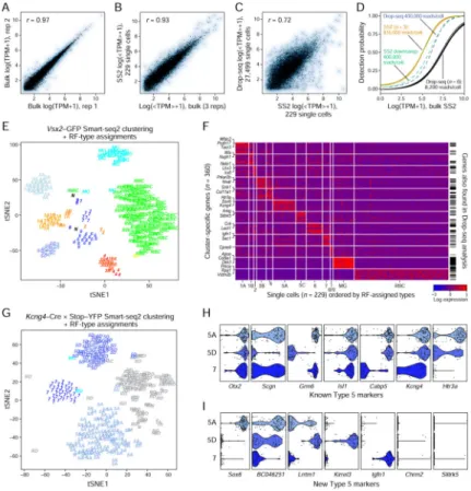
Could we have derived a better classification had we sequenced fewer cells at greater depth for equivalent cost? To explore this, we collected GFP+ cells from the Vsx2-GFP line and prepared 288 single-cell libraries using Smart-seq2, a near full-length RNA-seq method (Picelli et al., 2014) as well as bulk population libraries from ~10,000 GFP+ cells (Figure 7A–B). We analyzed 229 single cells that passed quality filters (Methods and Resources); they were sequenced to a median depth of 835,000 mapped reads per cell; the cumulative depth of these 229 libraries (mapped reads) was equivalent to 23,300 Drop-seq libraries or ~83% of our dataset. Gene expression profiles averaged across Smart-seq2 single cells, Smart-seq2 bulk and Drop-seq libraries were highly correlated (Figure 7B, C). However, the per-cell effective library+sequencing cost of the Smart-seq2 cells was $18 (55x greater than Drop-seq), such that the overall cost of 229 single cells was equivalent to ~12,200 Drop-seq cells (excluding time considerations and labor costs).
We assessed sensitivity of detection by computing the fraction of cells in which a gene was detected as a function of its population expression level. As expected, the higher sequencing depth per cell in Smart-seq2 enabled better detection of lowly expressed genes, compared to Drop-seq (Figure 7D). To test whether this was related to sequencing depth or was a limitation intrinsic to Drop-seq, such as low transcript capture on beads, we re-sequenced ~200 single-cell Drop-seq libraries at 50X greater depth (400,000 mapped reads per cell). Deeper sequencing greatly improved the transcript detection efficiency in Drop-seq libraries, and was comparable to Smart-seq2 libraries downsampled to a similar depth (Figure 7D).
A
uthor Man
uscr
ipt
A
uthor Man
uscr
ipt
A
uthor Man
uscr
ipt
A
uthor Man
uscr
ipt
We next examined the performance of fewer, deeply sequenced cells in cell type
identification. Clustering the 229 single cells using an approach similar to that used for the Drop-seq data generated only 8 clusters, many of which expressed signatures of multiple BC types (Figure 7E, Methods and Resources). We classified individual cells within these clusters using a random forest (RF) model (Figure 7E, labels) trained on Drop-seq bipolar signatures (Figure S3D, Methods and Resources). The predicted labels of individual cells showed that a majority of the mixed clusters were comprised of BC pairs that were each other’s closest relative (e.g. BC1A-1B, BC3B-4 and BC5B-5C). No cells were classified as BC3A or BC5D cells, likely because they were too rare to be captured in the dataset (1.7– 1.9 % in Drop-seq data). In contrast, these type were identified in Drop-seq datasets containing ~5000 shallow-coverage cells (Figures S2N, S3A). These results suggest that for the task of cell type identification greater sequencing depth per cell is insufficient to compensate for the underrepresentation of cell types.
Next, using the cell-type labels assigned by the RF model, we obtained the top 30 DE genes for each BC type in the Smart-seq2 data using a bimodal test (McDavid et al., 2013). 60% of these markers featured among the top 30 DE genes found in the Drop-seq analysis (Figure 7F), suggesting consistency between the results obtained from the Drop-seq and Smart-seq2 libraries. The proportion of gene discrepancies was larger for Smart-seq2 clusters with small numbers of cells, suggesting that these might be false positives.
To further test whether our ability to cluster Smart-seq2 data was limited by numbers of cells, we prepared Smart-seq2 libraries of YFP-positive BCs from retinas of Kcng4-Cre mice crossed to a stop-YFP Cre-dependent reporter. (Methods and Resources). Unbiased clustering of 309 cells identified four large clusters in the data, three of which corresponded to BC5A (n=110), BC5D (n=60), and BC7 (n=43) based on the RF model (Figure 7G–I; labels), consistent with Kcng4 expression (Figure 1F). A fourth cluster (n=82) consisted of likely rod-BC5 doublets; the RF model assigned classes for <10% of the cells in this cluster. Together, these results demonstrate the importance of distributing a given number of reads over a large number of cells in order to accurately resolve cell types.
DISCUSSION
We developed and applied an integrated strategy for building a comprehensive validated atlas of cell types. Challenges included (1) the need to harmonize different definitions of cell type (here, molecular and morphological); (2) a population containing both abundant and rare cell types; (3) the need for a scalable and robust computational approach; and (4) the need to optimize the depth of profiling and the number of profiled cells, given fixed resources. We showed that our classification is comprehensive in covering all known mouse BC types, and that associated transcriptional profiles are accurate, identifying the majority of known markers and new ones that we went on to validate. We also discovered two BC types not previously identified and generated an extensive resource for future studies. Finally, we provide an experimental and computational framework for similar studies in other systems.
A
uthor Man
uscr
ipt
A
uthor Man
uscr
ipt
A
uthor Man
uscr
ipt
A
uthor Man
uscr
ipt
BCs are an ideal class for cell type analysis
We used BCs to develop and test our strategy for several reasons. First, BC types have been classified morphologically at both light and electron microscopic levels (Helmstaedter et al., 2013; Wassle et al., 2009). Second, BCs are readily accessible by viral infection, and we employed lentiviral vectors for sparse, random labeling of BCs; combined with FISH, this allowed us to relate candidate marker expression to the morphologies of BC types. Third, endogenous and transgenic markers were already available for some BC types, aiding the assignment of cell clusters to BC types and allowing us to assess the accuracy of
computational approaches at an early stage of the analysis. BC types, markers, factors and relationships
The discovery of BC1B illustrates the power of scRNA-seq. BC1B cells appeared amacrine-like in morphology and position, and indeed may have been misclassified as amacrine cells in previous studies. However they display a typical bipolar morphology during development, and remain molecularly bipolar-like in adulthood (Figure 3). Such morphological transitions during development have precedents within the CNS. In the mammalian cortex, for example, some pyramidal neurons retract their apical dendrite and become spiny stellate neurons (Koester and O’Leary, 1992). Such examples raise the possibility that some morphology-based classifications of neuronal types will be revised with the application of molecular profiling.
Hierarchical clustering of BC types based on transcriptional profiles provides insight into the relationships among BCs. The two main distinctions among BC types are rod vs. cone BCs and ON vs. OFF BCs. The former is associated with synaptic input (predominantly from rod vs. cone photoreceptors), while the latter distinguishes the signaling mechanism in dendrites (metabotropic vs ionotropic; Figure 6D) and the level of axonal stratification. The first split in the dendrogram (Figure 6B) separates the rod from cone BCs, with a second split
separating ON cone from OFF cone BCs. Thus, ON cone BCs are more similar to OFF cone BCs than to ON rod BCs.
Grouping of cone BC clusters also shows that lamination depth in the IPL correlates well with molecular relatedness. Although BC5D uniquely shares a wide axonal arbor morphology with BC8 and 9, it does not show a close transcriptional relatedness to these types. Rather, the four clusters with cells that co-laminate, BC5A–D, were grouped together despite their varied arbor morphologies (Figure 6A, B). Likewise, BC6–9, which laminate lower in the IPL, were positioned together in the dendrogram.
One possible exception to this rule is BC2. Despite sharing lamination with BC1A and BC1B, BC2 did not cluster reliably with these types, with only 70% of the bootstrap trials placing it in the OFF BC branch. In a large proportion of the other trials it was positioned in the ON branch next to BC6. Interestingly, BC2 expresses genes encoding components of the ON-type glutamate receptor signaling complex (Gng13, Nyx, and Trpm1) (Figure 6D).
A
uthor Man
uscr
ipt
A
uthor Man
uscr
ipt
A
uthor Man
uscr
ipt
A
uthor Man
uscr
ipt
Design considerations for scRNA-seq based cell classification
Although each system will surely present its own challenges, we believe our work presents a starting point for designing studies aimed at classifying other heterogeneous tissues.
First, our success in classifying BCs using shallow-sequenced Drop-seq libraries supports previous studies (Heimberg et al., 2016; Jaitin et al., 2014; Macosko et al., 2015; Pollen et al., 2014), which have noted that the majority of genes that account for transcriptional variance between cell types are identifiable by low coverage RNA-seq (10–50,000 reads per cell). To this we add evidence that shallow sequencing can be used for comprehensive classification. Drop-seq is also cost-effective: At $0.34/cell, Drop-seq datasets of 13,938 cells ($4,739) enabled better cell type classification than Smart-seq2 (229 cells × $18/cell= $4,122) (Figures 7, S2). However, more depth may be required in systems where cell type distinctions are graded (e.g., developing tissues), or when dynamic processes are being monitored. An attractive strategy would be to first identify cell types using large numbers of cells profiled at shallow depth, and then, if desired, re-sequence a subset at higher coverage for a deeper analysis (Figure 7D).
Second, our analysis of downsampled Vsx2-GFP Drop-seq, and Smart-seq2 datasets (Figures 7, S2, S3) underscores the importance of large cell numbers for robust
classification. Retrospectively, we were able to resolve BC types occurring at a frequency >200 cells in the Drop-seq datasets (Table S2). Some non-BC types, like cone
photoreceptors, were resolvable at <50 cells per cluster, presumably because of their transcriptional distinctness. Thus, the minimum number of cells needed to resolve all cell types is a function of their frequency distribution, transcriptional distinctness, and depth of sequencing. In particular, comparison of Vsx2-GFP Drop-seq and Smart-seq2 data shows that deeper sequencing does not enable better classification when cell numbers are low. For example, BC3B and BC4 could not be resolved from each other in Smart-seq2 data even though their proportions were higher in the Smart-seq2 dataset (4.4%, 3%) than in Drop-seq (2.9%, 1.4%). The computational challenges separating the two rarest BC types, BC8 and BC9, in the Drop-seq data at various levels of cell downsampling further underscores the need for large cell numbers in classifying rare, related types.
Third, with the advance of multiplexing technologies and decreasing sequencing costs, future studies will undoubtedly profile larger numbers of cells at greater depth. Analysis of such datasets will require scalable computational methods. We tested six clustering methods, of which two, Louvain-Jaccard (Blondel et al., 2008) and Infomap (Rosvall and Bergstrom, 2008), produced the most useful results. Both methods have an approximately linear complexity with the number of cells, making this approach promising for large scRNA-seq datasets in the future. The tradeoff between the two methods (sensitivity vs. over-clustering) exposes the challenges inherent to clustering, and suggests that future studies aimed at classifying less well-characterized regions of the brain would benefit from analyzing data using multiple clustering approaches, followed by additional validations of putative types.
A
uthor Man
uscr
ipt
A
uthor Man
uscr
ipt
A
uthor Man
uscr
ipt
A
uthor Man
uscr
ipt
What defines a cell type?
Most neurobiologists agree that classifying the cell types of the nervous system is essential for understanding how the brain develops, functions, and malfunctions. There is less agreement, however, on how to define a cell type. In C. elegans, the task is straightforward: each neuron can be viewed as a type, with a unique lineage, position, pattern of connectivity, molecular profile and functions. In the vertebrate nervous system, with orders of magnitude more neurons (~1011 in the human brain), it is more difficult to define a type. One hopes for a taxonomy that meaningfully reconciles morphological, physiological, molecular and perhaps other criteria (e.g., position, connectivity).
It is encouraging that correspondence among these criteria seems to be the rule for BCs. It is unclear, however, whether distinctions will be as crisp for other populations, such as neurons of the cerebral cortex, where activity and other factors can profoundly affect neuronal properties (Spitzer, 2015), and intermediate types may exist (Tasic et al., 2016). Indeed, molecular classifications are likely to fail if they do not take account of activity- and state-dependent transcriptional programs. Nonetheless, we argue that comprehensive
transcriptomic classification using large numbers of cells, coupled with extensive validation, provides a useful starting point for generating neuronal taxonomies.
Methods Text
CONTACT FOR REAGENT AND RESOURCE SHARING
Further information and requests for reagents may be directed to, and will be fulfilled by the corresponding author Joshua R. Sanes ([email protected]).
EXPERIMENTAL MODELS AND SUBJECT DETAILS
MICE—All animal experiments were approved by the Institutional Animal Care and Use Committees (IACUC) at Harvard University. Mice were maintained in a specific pathogen free facility under standard housing conditions with continuous access to food and water. All RNAseq experiments were carried out at post-natal age (P) 17. Histological studies used P17-60 mice unless indicated otherwise. Male and female mice were used across different experiments. None of the mice had noticeable health or immune status abnormalities, and were not subject to prior procedures. The genotype of mice are described where appropriate. The following mouse lines were used:
1. Tg(Chx10-EGFP/cre,-ALPP)2Clc transgenic mice (Vsx2-GFP hereafter) were bred for two generations to CD1 (Charles River) and used for FACS experiments of GFP-positive cells (Rowan and Cepko, 2004).
2. Transgenic Clomeleon-1 (CLM1) mice, which encode a topaz-cyan fusion fluorescent indicator protein under control of a Thy1 promoter, were used to visualize blue cone BCs (gift of Dr. Kevin Staley) (Berglund et al., 2006).
3. Transgenic Gustducin-GFP (Tg(GUS8.4GFP)) mice were used to identify BC7 cells (Huang et al., 2003; Huang et al., 1999).
A
uthor Man
uscr
ipt
A
uthor Man
uscr
ipt
A
uthor Man
uscr
ipt
A
uthor Man
uscr
ipt
4. A knock-in of membrane localized EGFP to exon 1 of Kirrel3
(Kirrel3tm1.1Jfcl) was used at P21 to visualize BC5D cells (gift of Dr. Jean-François Cloutier) (Prince et al., 2013).
5. Kcng4tm1.1(cre)Jrs mice (Duan et al., 2014) were crossed to the cre-dependent reporter Thy1-stop-YFP Line#1 (Buffelli et al., 2003) and used for FACS experiments of YFP-positive cells for single cell Smart-seq2 and immunohistochemistry (IHC) (hereafter Kcng4-cre;stop-YFP).
6. Mice expressing tau-lacZ under the endogenous Cntn5 locus
(Cntn5tm1Kwat) and used for AAV-stop-GFP infections at P3 or IHC at P113 (Li et al., 2003).
7. Ccktm1.1(cre)Zjh mice were used for AAV-stop-GFP infections at P0 (gift of Dr. David Ginty) (Taniguchi et al., 2011).
8. Thy1-mitoCFP-P (MitoP) mice express CFP under the control of a Thy1 promoter in neuronal mitochondria, and labels BC1A, BC1B, and nGnG amacrine cells (Kay et al., 2011; Misgeld et al., 2007; Schubert et al., 2008). These mice were used for FISH and/or IHC at P6, 8, 11, 17, and P100.
9. BC1B cells were also visualized by IHC at P56 using
Fezf1tm1.1(cre/folA)Hze mice crossed to a td-Tomato cre-reporter
Gt(ROSA)26Sortm14(CAG-tdTomato)Hze (Madisen et al., 2010) (gift of the Allen Brain Research Institute).
10. Transgenic mice expressing EGFP under a Htr3a promoter (Tg(Htr3a-EGFP)#aShkp) were used for FACS followed by bulk RNA-seq (Haverkamp et al., 2009). These mice were also crossed to Kcng4tm1.1(cre)Jrs and retinas were used for IHC at P20. 11. Mice with lacZ knocked-in to the Cdh9 locus were crossed to
Kcng4tm1.1(cre)Jrs mice and used for IHC at P20 (Duan et al., 2014). METHOD DETAILS
RNA-SEQUENCING
Isolation of cells for sequencing: For Drop-seq experiments using the Vsx2-GFP line, retinas were dissected in Hank’s balanced salt solution (HBSS) and promptly dissociated using an accelerated DNAse-free dissociation protocol (Siegert et al., 2012) with minor modifications. Papain (Worthington, LS003126) was removed with one wash in 10% FBS in HBSS followed by one wash in DMEM, after which retinas were placed in DMEM
containing 0.4% BSA (Sigma, A8806), dissociated by trituration, passed through a 35μm cell strainer, and placed on ice. Propidium Iodide (0.01 mg/mL) was added as a dead cell stain. Cells from Vsx2-GFP negative littermates were used to determine background fluorescence levels, and cells above this threshold from Vsx2-GFP positive animals were collected using FACS into PBS plus 0.1% BSA at a concentration of 100 cells/μl and 1 ml
A
uthor Man
uscr
ipt
A
uthor Man
uscr
ipt
A
uthor Man
uscr
ipt
A
uthor Man
uscr
ipt
aliquots were used as input to the Drop-seq protocol. Cells were processed for Drop-seq within ~30 minutes of collection.
For Smart-seq2 experiments using the Vsx2-GFP line, three individual retinas from two animals were dissected, dissociated, and FAC sorted as above. Single cells from each retina were collected into separate 96-well plates with 5 μl lysis buffer comprised of Buffer TCL (Qiagen 1031576) plus 1% 2-mercaptoethanol (Sigma 63689). We also collected ~10,000 cells from each retina into 350 μl lysis buffer to serve as population RNA-seq controls. All samples were immediately frozen at −80°C.
To identify BC types marked by the Kcng4-cre line, mice were crossed to the cre-dependent reporter Thy1-stop-YFP and YFP-positive single cells were FAC sorted as described above in the Vsx2-GFP Smart-seq2 experiments, with some minor differences in retinal
dissociation. Briefly, individual retinas from two P17 Kcng4-cre;stop-YFP mice were dissected in ice-cold HBSS, digested with papain for 5 minutes, washed with Ovomucoid solution (Worthington, LS003087) to inactivate papain, dissociated by manual trituration, and passed through a 40 μm cell strainer. To exclude retinal ganglion cells (RGCs) that are also marked in Kcng4-cre;stop-YFP retinas (Duan et al., 2015) dissociated cells were incubated with a pan-RGC cell surface marker, anti-mouse CD90.2 (Thy-1.2) PE-Cyanine7 (Affymetrix, 25-0902-81) (Kay et al., 2012). During FAC sorting, only YFP+ Cy7− BCs were collected, and YFP+ Cy7+ RGCs were excluded.
Drop-seq procedure: Drop-seq was performed largely as described previously (Macosko et al., 2015). Briefly, cells were diluted to an estimated final droplet occupancy of 0.05, and co-encapsulated in droplets with barcoded beads, which were diluted to an estimated final droplet occupancy of 0.06. The beads were purchased from ChemGenes Corporation, Wilmington MA (catalogue number Macosko201110). Individual droplet aliquots of 2 mL of aqueous volume (1 mL each of cells and beads) were broken by perfluorooctanol, following which beads were harvested, and hybridized RNA was reverse transcribed. Populations of 2,000 beads (~100 cells) were separately amplified for 14 cycles of PCR (primers, chemistry, and cycle conditions identical to those previously described) and pairs of PCR products were co-purified by the addition of 0.6x AMPure XP beads (Agencourt). A total of six replicates were prepared from two experimental batches (Batch 1 and Batch 2) of FAC sorted Vsx2-GFP positive cells on different days. For each batch, retinas from multiple littermates were pooled together. Batch 1 consisted of cells from 5 mice, whose cells were divided into 4 replicates and Batch 2 consisted of 4 mice, whose cells were split into 2 replicates. Each replicate was collected by Drop-seq from 1 ml FAC sorted GFP-positive cells pooled from multiple Vsx2-GFP mice. For Batch 1 replicates 1–4, cDNA from an estimated 5,400 cells were prepared and tagmented by Nextera XT using 600 pg of cDNA input, and the custom primers P5_TSO_Hybrid and Nextera_N701 (see table below). For Batch 2 replicates 1–2, cDNA from an estimated 11,700 cells was used as input into the Nextera XT tagmentation. Each replicate was separately sequenced on the Illumina NextSeq 500 using 1.8 pM in a volume of 1.3 mL HT1, and 3 mL of 0.3μM Read1CustSeqB (see table below) for priming of read 1. Read 1 was 20 bp; read 2 (paired end) was 60 bp.
A
uthor Man
uscr
ipt
A
uthor Man
uscr
ipt
A
uthor Man
uscr
ipt
A
uthor Man
uscr
ipt
Template_Switch_Oligo AAGCAGTGGTATCAACGCAGAGTGAATrGrGrG
TSO_PCR AAGCAGTGGTATCAACGCAGAGT
P5-TSO_Hybrid AATGATACGGCGACCACCGAGATCTACACGCCTGTCCGCGGAAGCAGTGGTATCAACGCAGAGT*A*C Nextera_N701 CAAGCAGAAGACGGCATACGAGATTCGCCTTAGTCTCGTGGGCTCGG
Read1CustomSeqB GCCTGTCCGCGGAAGCAGTGGTATCAACGCAGAGTAC
To sequence a smaller number of Drop-seq libraries at a greater depth (Figure 7D), amplified cDNA from approximately 200 single-cell profiles from replicate 4 of Batch 1 was
tagmented by the above Nextera XT protocol. This library was sequenced in a separate Illumina NextSeq 500 run using the same recipe as above.
Plate-based RNA-seq experiments: For preparation of single-cell libraries from 96-well plates (for Vsx2-GFP and Kcng4-cre;stop-YFP cells), we thawed the cells and purified them with 2.2x RNAClean SPRI beads (Beckman Coulter Genomics,) without final elution. The RNA captured beads were air-dried and processed immediately for cDNA synthesis. We performed Smart-seq2 following the published protocol (Picelli et al., 2014) with minor modifications in the reverse transcription (RT) step (Monika Kowalczyk, in preparation). We made 25 μl reaction mix for each PCR and performed 21 cycles for cDNA amplification. We used 0.075 ng cDNA of each cell and ¼ of the standard Illumina NexteraXT reaction volume in both the tagmentation and final PCR amplification steps.
For the bulk RNA samples from the Vsx2-GFP line, we purified total RNA using the RNeasy Mini Kit (Qiagen, 74104) with the in-column DNase treatment step. We used 1 ng total RNA and made Smart-seq2 libraries as for the single cells described as above, except only 12 cycles PCR for cDNA amplification.
We pooled the 288 single-cell libraries and 3 bulk sample libraries from the Vsx2-GFP line, and sequenced 50 × 25 paired-end reads using a single kit on the NextSeq500 instrument. The 396 Kcng4-cre single cell libraries were sequenced on two lanes of the HiSeq2500 instrument with 50bp single end reads (192 libraries per lane).
For bulk sequencing experiments using the Htr3a-GFP line we collected 15,000 GFP-positive cells into RNAlater (ThermoFisher, AM7024) in two replicates. RNA was purified using ARCTURUS PicoPure columns (ThermoFisher, KIT0204). Reverse transcription and cDNA amplification was performed using the Ovation RNA-seq system V2 (Nugen, 7102-32).
Cost-model for Drop-seq and Smart-seq2
Drop-seq: The 45,000 cells profiled using Drop-seq were sequenced on six lanes of
Next-seq (~8,200 mapped reads per cell). Based on a library generation cost of 6c / cell and $1,100 per Next-seq kit, the cost of 45,000 single-cell libraries was $9,300. For 27,499 cells that passed QC filters, this yielded an effective per-cell cost of 34c / cell.
A
uthor Man
uscr
ipt
A
uthor Man
uscr
ipt
A
uthor Man
uscr
ipt
A
uthor Man
uscr
ipt
Smart-seq2: The 288 cells profiled using Drop-seq were sequenced on a single lane of
Next-seq (~835,000 mapped reads per cell). Based on a library generation cost of $10.27 / cell, the cost of 288 single cell-libraries was $4058, yielding a cost of $17.8 / cell for the 229 cells that passed QC filters.
The effective cost of sequencing 27,499 Drop-seq libraries to an equivalent depth of our Smart-seq2 libraries is $23.5/cell (100x deeper), slightly larger than the cost of a Smart-seq2 library, because a higher proportion of reads are lost in Drop-seq to barcode errors and cellular debris. We note, however, that this calculation does not take into account labor costs and preparation time, both of can be substantially higher for Smart-seq2 compared to Drop-seq for an equivalent number of libraries
HISTOLOGICAL METHODS
Probe generation and fluorescent in situ hybridization: Probe templates were generated using cDNA derived from P17 CD1 mouse retina following RNA extraction and reverse transcription with Superscript III (ThermoFisher, 18080051). Antisense probes were generated by nested PCR, with the second PCR using a reverse primer with a T7 sequence adapter to permit in vitro transcription (see Table S4 for primer sequences). DIG rUTP (Roche, 11277073910) was used for synthesis of probes for all single FISH experiments, and DNP rUTP (Perkin Elmer, NEL555001EA) was used for double FISH probes. FISH on sectioned tissues was performed as described (Trimarchi et al., 2007), with modifications. Freshly dissected retinas were fixed in 4% PFA in PBS at room temperature for 30 minutes and immediately embedded in 1:1 30% sucrose:OCT. Sections were adhered to Superfrost slides, treated with 1.5 μg/ml of proteinase K (NEB, P8107S) and then post-fixed and treated with acetic anhydride for deacetylation. Probe detection was performed with anti-DIG HRP (1:750) or anti-DNP HRP (1:200) followed by tyramide amplification. Detection of protein epitopes was performed following probe detection. Antibodies were diluted in block consisting of 3% donkey serum (Jackson, 017-000-121), 1% BSA, and 0.1% Triton-X in PBS at concentrations of 1:1000 (anti-Calretinin and anti-PkarIIb), 1:500 (anti-GFP), and 1:1500 (anti-PKCα) (See below for antibody information). For whole mount FISH, retinas of CD1 mice (age P25) were fixed in 4% PFA, freeze-thawed in 30% sucrose, and then treated with PBS + 0.3% Triton-X for 30 minutes prior to proteinase K treatment (5 μg/ml). Here, blocking steps were performed with Triton-x (0.3%).
Modified lentivirus for single BC labeling: The FUGW lentiviral genome plasmid (Lois et al., 2002) was used as the backbone to insert an element upstream of the Vsx2 (Chx10) gene that drives expression in BCs and Müller glia. This element is the chicken homolog of a previously described mouse enhancer (Emerson and Cepko, 2011), and was PCR amplified from genomic DNA using primers (5′TTAAGATAACGTACACACACAGCGT3′ and 5′CGAGTAAAATGTCTTCCCCGCAGC3′) and placed upstream of an SV40 promoter followed by GFP (amplified from Addgene plasmid #18808) (Kim et al., 2008a). We call this plasmid FChxVGW. Virus was generated by transfection of 293T cells with the
FChxVGW genome plasmid, pspax2 packaging plasmid (Addgene #12260) and an envelope expressing plasmid, CMV-VSV-G. 10 μg of DNA was transfected per 10 cm plate, in a plasmid ratio of 6:3:1 genome:packaging:envelope, and 48 and 72 hour supernatants were
A
uthor Man
uscr
ipt
A
uthor Man
uscr
ipt
A
uthor Man
uscr
ipt
A
uthor Man
uscr
ipt
concentrated by ultracentrifugation. CD1 pups were injected subretinally at P1 and infected retinas were harvested at P17–P20 for FISH and IHC.
Cre-dependent AAV for single BC labeling: Sparse labeling of BCs was also achieved using an adeno-associated virus (AAV) expressing fluorescent proteins in a cre-dependent manner. Brainbow virus AAV9.hEF1a.lox.TagBFP.lox.eYFP.lox.WPRE.hGH-InvBYF (titer: 1e12) (Penn Vector Core, AV-9-PV2453) (Cai et al. 2013) was injected into the sub-retinal space of Kcng4-cre;Cntn5-tau-lacZ and Cck-cre newborn mouse pups, and eyes were collected three weeks later and retinas dissected out and either maintained as retinal whole-mounts or cryosections prior to IHC.
Immunohistochemistry: Animals were given a lethal dose of sodium pentobarbital (120 mg/kg) (MWI, 710101) and either enucleated immediately or perfused intracardially with 4% PFA. Eye were removed and fixed in PFA for 15–30 minutes. Following dissection, retinas were either kept whole or immersed in 30% sucrose overnight prior to freezing in TFM (EMS, 72592) and cryosectioning at 20 μm. Immunostaining of retinal whole-mounts and cryosections was conducted as described previously (Duan et al., 2014; Krishnaswamy et al., 2015). Primary antibodies used: mouse anti-β-galactosidase (DSHB, 40-1a), rabbit anti-β-galactosidase (Duan et al., 2014), rabbit anti-calretinin (Millipore, AB5054), mouse anti-calretinin (Milipore, AB1568), goat anti-ChAT (Milipore, AB144P), goat anti-Chx10 (Santa Cruz Biotechnology, 21690), sheep anti-Chx10 (Exalpha, X118OP), mouse anti-cre (Milipore, AB3120), chicken anti-GFP (Abcam, ab13790), rabbit anti-Lhx3 (gift of Dr. Sam Pfaff) (Sharma et al., 1998), rabbit mcherry (Krishnaswamy et al., 2015), rabbit anti-Nfia (Active Motif, 39397), Rabbit anti-Otx2 (Millipore, AB9566), mouse anti-PkarIIb (BD Bioscience, 610625), rabbit anti-PKC (Sigma, P4334), rabbit anti-Ppp1r17 (Atlas
Antibodies, HPA047819), mouse anti-Syt2 (ZIRC, Znp-1). All secondary antibodies used were purchased from either Invitrogen or Jackson ImmunoResearch.
Image collection, processing, and analysis: Images were collected using several scanning laser confocal microscopes, including an Olympus Fluoview 1000, Ziess LSM 710, or Ziess LSM 780. ImageJ, Zen, and Imaris software were used to generate maximum projections and rotations of image stacks, and Adobe Photoshop CC was used for adjustments to brightness and contrast. ImageJ was also used for noise reduction. IHC for GFP following FISH occasionally caused the appearance of bright puncta. These background speckles obscured the visualization of lentivirus labeled cells. Therefore, we applied the ‘Remove outliers’ noise filter process in ImageJ to the GFP channel only in lentivirus+FISH images. This process replaces a pixel if it deviates from the median of the surrounding pixels by a given value. A pixel radius of 3 or less and the default threshold of 50 were used to remove bright outliers. No aspects of cell morphology were detectably obscured after applying the filter. The BC1B bipolar to unipolar transition was quantified from MitoP retinal sections stitched together using the pairwise stitching plugin of ImageJ (Preibisch et al., 2009). WinDRP (http://wvad.mpimf-heidelberg.mpg.de/abteilungen/biomedizinischeOptik/ software/WinDRP/index.html) was used to generate density recovery profiles and calculate the effective radius for real and density matched random populations of BC5D and BC9.
A
uthor Man
uscr
ipt
A
uthor Man
uscr
ipt
A
uthor Man
uscr
ipt
A
uthor Man
uscr
ipt
COMPUTATIONAL METHODS FOR DROP-SEQ DATA Preprocessing of Drop-seq data
Read filtering and alignment: Paired-end sequence reads were processed largely as
described before (Macosko et al., 2015) with an additional barcode correction step (see below). Briefly, the left read was used to infer the cell of origin based on the first 12 bases (the cell barcode or CB), and the molecule of origin based on the next 8 bases (Unique molecular Index or UMI). Reads were first filtered to remove all pairs where either the CB or the UMI had one or more bases with quality score less than 10. The right mate of each read pair (60 bp) was trimmed to remove any portion of the SMART adapter sequence or large stretches of polyA tails (6 consecutive bp or greater). The trimmed reads were then aligned to the mouse genome (version m38) using STAR v2.4.0a (Dobin et al., 2013) with the default parameter settings. Reads mapping to exonic regions of genes as per the Ensembl transcriptomic annotation (version 81) were recorded. Exonic reads that mapped to multiple locations or to the antisense strand were discarded.
Correcting for barcode synthesis errors: During the analysis of our experimental data, we
noticed that our recently purchased batch of beads contained a sizeable fraction of cell barcodes (~5–10 %) that shared the first 11 bases, but differed at the last base. These CBs also had a very high fraction of “T” (>95%) at the last position of the UMI (see figure below). We concluded that these represented beads that were missing a single base of the CB, likely because they missed one of twelve split-and-pool synthesis cycles. Thus, for these beads, the 20-bp barcode read would be expected to contain a mixed base at position 12 (the first base of the UMI) and a fixed T at position 20 (the first base of the polyT segment). If uncorrected, this would lead to an overestimation of the true number of cells in the data (i.e., reads that have arisen from the same cell would be split to different “virtual” cells, because one position is not in fact part of the cell barcode, but rather the UMI).
To correct for this phenomenon, we first identified CBs with “fixed” UMI bases at position 12. If only the last UMI base is fixed as a “T”, we collected all the reads carrying cell barcodes that had an identical sequence at the first 11 bases, and “merged” these barcodes together. Empirically, we found that in these barcodes, “A”, “G”, “C” and “T” occurred in roughly equal proportions at base 12, consistent with our hypothesis that this was actually the first UMI base. We then made this the first UMI base by inserting an “N” at CB position 12 (denoting the missing base), and trimmed off the “T” at the last UMI base. If any other UMI base was fixed, all the reads carrying that CB were discarded. This resulted in a corrected set of cell barcodes and UMIs that was used for the estimation of digital gene expression. 5–10% of cell barcodes were corrected in this way in all the six replicates.
A
uthor Man
uscr
ipt
A
uthor Man
uscr
ipt
A
uthor Man
uscr
ipt
A
uthor Man
uscr
ipt
Histogram of the fraction of ‘T’ bases in the last UMI position for each cell barcode. Data from replicate 1 of Batch 1 of Drop-seq was used. For most cell barcodes (green), the fraction of ‘T’ at position 8 of the UMI barcode is drawn from a normal distribution centered around 0.25, consistent with a uniform distribution for all 4 bases. For a small number of the cell barcodes (~5%), a fixation of ‘T’ at the last UMI position is observed (blue).
A command line script to perform this correction has been made publicly available in the Drop-seq website (http://mccarrolllab.com/dropseq/), and its implementation is described in the Drop-seq computational cookbook (http://mccarrolllab.com/wp-content/uploads/ 2016/03/Drop-seqAlignmentCookbookv1.2Jan2016.pdf)
Digital gene expression: To distinguish cell barcodes that represent genuine transcriptomic
A
uthor Man
uscr
ipt
A
uthor Man
uscr
ipt
A
uthor Man
uscr
ipt
A
uthor Man
uscr
ipt
ordered the cell barcodes by the total number of transcripts per cell barcode and estimated a “shoulder” in the corresponding plot, as described before (Macosko et al., 2015). All cell barcodes larger than this cutoff were used in downstream analysis, while the remaining cell barcodes were discarded.
We then performed the following steps for every gene within every cell. The UMIs corresponding to all uniquely mapped sense reads (for a given gene) were recorded, and UMIs within an edit distance of 1 (substitutions only) were collapsed, as described in (Macosko et al., 2015). We then counted the number of remaining unique UMIs and this was recorded as the expression count for that particular gene in that particular cell. This resulted in a digital expression matrix (DGE) with genes as rows and cells as columns that served as the starting point for clustering analysis.
Batch correction, PCA analysis, tSNE visualization and clustering
Filtering the expression matrix: The starting pool of 45,000 cells (5,400 cells per replicate
in Batch 1 and 11,700 cells per replicate in Batch 2) was first filtered to remove cells where less than 500 genes1 were detected, and where the proportion of the transcript counts (i.e., UMIs) derived from mitochondrially encoded genes (e.g. Mt-Rnr2, Mt-Co2 etc.) was greater than 10%. We then removed genes that were detected in less than 30 cells, and also those that had fewer than 60 transcripts counts, summed across all the retained cells. These filters resulted in 27,499 cells and 13,166 genes, which were considered for further analysis. From Batch 1, we retained 3,055–3,851 cells from each of the four replicates. From Batch 2, we retained 7,129 cells and 6,383 cells from the two replicates, respectively (Figure S1A, Table S1).
Amongst the retained cells, the median number of genes detected per cell was 810 (IQR 644–1033, Figure S1A, upper panel) and the median number of transcripts counts was 1,192 (IQR 914–1607, Figure S1A, lower panel), and both these numbers were comparable across the different experimental batches and replicates. The median number of transcriptome-mapped reads per cell was 8,200. The median number of reads supporting each detected transcript was 4 (IQR 3–7), but this distribution was very wide (Figure S1B). 95% of non-zero gene-counts in the filtered matrix had a value less than or equal to 3 (75% 1’s, 16% 2’s and 4% 3’s), suggesting that our data (given the shallow sequencing depth) primarily reflected presence/absence of transcripts and did not capture the full dynamic range for most transcripts (Figure S1C).
Transcript counts within each column of the 13,166 genes × 27,499 cell count matrix were normalized to sum to the median number of transcripts per cell (1,192), resulting in normalized counts Mij for gene i in cell j. For PCA and clustering, we used a log-transformed expression matrix Eij = ln(Mij + 1).
QC metrics: A list of quality metrics was obtained for the Drop-seq single cell libraries
using Samtools (http://samtools.sourceforge.net/), Picard Tools (http://
broadinstitute.github.io/picard/) and in-house scripts. For each single cell library (identified based on its Batch, replicate and a 12bp barcode), we calculated the total number of mapped reads (coding and UTR), the number of genes detected per cell, percentage of the total
A
uthor Man
uscr
ipt
A
uthor Man
uscr
ipt
A
uthor Man
uscr
ipt
A
uthor Man
uscr
ipt
number of reads assigned to the cell barcode that were from (1) coding regions (2) UTRs (3) intronic regions (4) intergenic regions (5) ribosomal RNA, and (6) mitochondrially derived transcripts. These are summarized in Table S1.
Batch correction: Although the values of Eij between any two single cells correlated poorly, as expected (Figure S1D), the averaged expression levels of genes and the average counts were highly correlated across the six replicates (Figure S1E–H). However, we noted that the intra-batch correlations were slightly higher than the inter-batch correlations (Figure S1G, H). While no differentially expressed genes were detected between any two replicates from the same batch (e.g., Figure S1E, F), we detected 33 differentially expressed genes at an average expression fold change > 2 between the two batches (FDR < 0.05), most of them expressed at very low levels (see table below). These genes included Xist (the most differentially expressed), Tsix, Hopx and Eif2s3y, all of which are sex-related genes, and Egr1 and Jun, both early response genes to stress and injury. These observations suggest that differences in the proportion of males and females in the two litters, and differences in handling conditions between the two experiments, are therefore likely to contribute to these batch effects in gene expression.
Gene P-value log-fold change (Batch 1 vs Batch 2)
Xist < 1e-6 −3.14 BC033916 < 1e-6 1.87 2810008D09Rik < 1e-6 1.65 2700089E24Rik < 1e-6 1.65 Smim10l1 < 1e-6 −1.58 Platr17 < 1e-6 −1.56 A930011O12Rik < 1e-6 1.52 mt-Rnr2 < 1e-6 −1.37 Mir124a-1hg < 1e-6 −1.35 Hopx < 1e-6 1.34 Snhg20 < 1e-6 −1.29 Tsix < 1e-6 −1.29 Zfp638 < 1e-6 −1.24 Zfml < 1e-6 1.13 Eif2s3y < 1e-6 1.09 mt-Rnr1 < 1e-6 −0.99 RP23-102H7.9 < 1e-6 0.87 Rsrp1 < 1e-6 0.86 Eno1 < 1e-6 −0.86 Rpl26 < 1e-6 0.85 2510003E04Rik < 1e-6 0.85 Egr1 < 1e-6 −0.83