Field-scale estimation of the volume percentage of rock fragments in stony soils by electrical resistivity

(1)

HAL Id: hal-02652709

https://hal.inrae.fr/hal-02652709

Submitted on 29 May 2020

HAL is a multi-disciplinary open access archive for the deposit and dissemination of sci-entific research documents, whether they are pub-lished or not. The documents may come from teaching and research institutions in France or abroad, or from public or private research centers.

L’archive ouverte pluridisciplinaire HAL, est destinée au dépôt et à la diffusion de documents scientifiques de niveau recherche, publiés ou non, émanant des établissements d’enseignement et de recherche français ou étrangers, des laboratoires publics ou privés.

Field-scale estimation of the volume percentage of rock

fragments in stony soils by electrical resistivity

Marion Tetegan, Catherine Pasquier, Bernard Nicoullaud, Hocine

Bourennane, Arlène Besson, Caroline Desbourdes-Coutadeur, Alain Bouthier,

Dominique King, Isabelle Cousin

To cite this version:

Marion Tetegan, Catherine Pasquier, Bernard Nicoullaud, Hocine Bourennane, Arlène Besson, et al.. Field-scale estimation of the volume percentage of rock fragments in stony soils by electrical resistivity. CATENA, Elsevier, 2012, 92, pp.67-74. �10.1016/j.catena.2011.09.005�. �hal-02652709�

(2)

Version postprint Manuscri t d’auteur / Author Manuscri p t Ma nuscrit d’auteur / Au th or Manuscri p t Manus crit d’auteur / Author Man u scri p t

Version définitive du manuscrit publié dans / Final version of the manuscript published in :

Catena, 92, 67‐74

Estimating the volume percentage of rock fragments of a stony soil by electrical resistivity at the field scale

M. Tetegan a, b, C. Pasquier a, B. Nicoullaud a, H. Bourennane a, A. Besson a, c, C. Desbourdes-Coutadeur d, A. Bouthier b, D King a, I. Cousin a

a _{Institut National de la Recherche Agronomique, UR 0272 Science du Sol, 2163 Avenue de la Pomme de Pin,}

CS 40001 Ardon 45075 Orléans Cedex 2 – France

b

ARVALIS – Institut du Végétal, Domaine expérimental du Magneraud 17700 Saint Pierre d’Amilly – France

c

Institut National de la Recherche Agronomique, UMR LISAH, 2 place Pierre Viala, 34060 Montpellier cedex 1 – France

d

ARVALIS – Institut du Végétal, 45 voie Romaine, 41240 Ouzouer le Marché – France

Abstract

Analysing the properties and functional characteristics of heterogeneous soils containing several phases requires a correct estimation of the volume proportion of each phase. In the case of stony soils, the volume percentage of the content of rock fragments remains difficult to estimate in situ. This paper presents a method that uses field spatial electrical resistivity measurements to determine the volume proportion of rock fragments. Based on the hypothesis that the electrical resistivity signal noise increases as the proportion of rock fragments increases, a model was developed that uses the standard deviation of the apparent electrical resistivity measurements over a small area as an indicator of rock fragment contents. The model was tested on three study areas of several hectares containing soil units with varying quantities of rock fragments. The estimation of the rock fragment content was accurate, and the error estimation of about 6 % was the same order of magnitude as the Bussian model (1983). The developed model strongly depends on the water content in the soil and the rock type and must be calibrated in each context. Nevertheless, estimations of the rock fragment content in stony soils can be performed efficiently in the surface horizon as well as all along the soil profile.

(3)

Catena, 92, 67‐74

I. Introduction

Currently, it remains difficult to provide estimates of the hydraulic properties of stony soils at the regional scale. To avoid bias, the hydraulic properties of stony soils must account for the presence of both rock fragments and fine earth, i.e., the characteristic individual hydraulic properties, and their volume content (Cousin et al., 2003; Tetegan et al., 2011; Ugolini et al., 1998). The estimation of the volume content of rock fragments is challenging although several methods have been used for a long time. For instance, estimates of rock fragment content can be measured from the soil surface reflectance by remote sensing; this method distinguishes among soil types and soil surface conditions, such as soil micro topography and vegetation cover (Girard and Girard, 2003). Other studies have demonstrated that a relationship exists between the percentage of rock fragments and the brightness index (Bhattacharya and Chandrakar, 1999; Mathieu et al., 2007; Post et al., 1999). However, this method strongly depends on the colours of the rock fragments and the soil conditions. Indeed, directly following a rain, the presence of the cleaned rock fragments is easier to detect. In contrast, after ploughing, the fine earth embedding the rock fragments can introduce a bias into the estimation of the volume content of rock fragments.

The rock fragment content of the deepest soil layers can be estimated by invasive methods, such as soil sampling. Soil sampling requires digging a pit, and large volumes of soil, i.e., large enough to be representative of the soil particle size distribution, must be sampled in each soil horizon and sieved. A visual estimation can also be performed with a chart, but this method strongly depends on the operator (Folk, 1951; Jeffrey, 1985; Terry and Chillingar, 1955). Thus, a real challenge still exists in terms of estimating the rock fragment content along a soil pit without disturbing the soil.

Geoelectrical methods, such as electrical resistivity profiling, are non-invasive methods that are useful for characterising the spatial variability in soils (Samouëlian et al., 2005; Sudduth et al., 2001). Variations in electrical resistivity result from differences in soil textures, soil structure and some other physical soil properties, including the moisture content and bulk density of the soil (Besson et al., 2004; Seger et al., 2009). However, the electrical resistivity method requires good contact between the soil and electrodes to facilitate the injection of a direct electrical current into the soil. Faulty electrodes can introduce noise into a dataset, i.e., unexpected zero values or very high values. In particular, this noise arises from i) measurement errors due to the measuring device, ii) sporadic errors due to external effects (Tabbagh, 1988) and iii) poor electrode contact that can occur frequently in dry and stony soils.

The presence of rock fragments can strongly affect the electrical signal. Rock fragments located at the soil surface are responsible for noise in the measurement dataset due to interference with electrode/soil contact. In addition, the resistivity of rock fragments is generally higher than the resistivity of fine earth by several orders of magnitude (Schon, 1996; Telford et al., 1976). Several laboratory experimental studies have been conducted to study the electrical properties of rocks (Guichet, 2002; Marescot, 2006; Olhoeft, 1981;

(4)

Catena, 92, 67‐74

Parkhomenko, 1967; Schon, 1996; Telford et al., 1976). Experimental measurements by Rey et al. (2006) on two-phase heterogeneous media consisting of resistive inclusions embedded in a conductive matrix demonstrated the validity of the model of Bussian (1983) for estimating the volume proportion of rock fragments in the soil. Following these promising experiments, we propose using electrical resistivity data to estimate the volume percentage of rock fragments at the field scale.

The aim of this study was to test the efficiency of the electrical resistivity method for estimating the rock fragment content of soil at the field scale. This analysis was based on two methods. The first method is an application of the model of Bussian (1983) that was previously used by Rey et al. (2006). The second method focuses on noise data extracted from spatial unfiltered electrical resistivities of soil. These geophysical methods were compared to those usually used in the field, visual descriptions from a cartographic survey and measurements of the volume content of rock fragments after soil sampling.

II. Materials and methods

4.1 Study area

The study area was located in the Beauce region (Villamblain, France) about 110 km southwest of Paris. It extended over an area of 115 hectares and was generally cropped with maize and wheat (Nicoullaud et al., 2004). The climate was temperate continental with an oceanic influence and was characterised by an average temperature of 10.5°C, a modal rainfall of about 623 - 630 mm and an evapotranspiration of about 767 - 783 mm (Besson, 2007; Michot, 2003a; Michot, 2003b). These mean values were calculated over a period of 32 years (1967 to 1996), and the evapotranspiration was calculated using the Penman-Monteith formula. In 1995, i.e., prior to geophysical surveys, 290 auger holes were dug to develop a description of the soils in the study area. The information obtained from the auger holes was used to establish a soil database for the study area. The soils consisted of a loamy-clay layer (about 60% loam and 30% clay) developed over lacustrine limestone deposits, which were locally cryoturbed. The thickness of this loamy-clay layer varied between 0.2 and 0.9 m. According to i) the spatial variability of the soil characteristics, ii) the depth and type of limestone where soil horizons were developed and iii) the thickness of the loamy-clay layer, the study area was classified into eight main soil units (Nicoullaud et al., 2004; Besson et al., 2010). These units were mainly haplic calcisols and calcaric cambisols (IUSS Working Group WRB, 2006) containing various quantities of rock fragments with different sizes, from gravels to blocks. As described by King et al. (1999) and Bourennane et al. (1998), the soil units formed on cryoturbed limestone deposits or on soft limestone deposits had the deepest loamy-clay layer (up to 0.8 m deep), whereas the shallowest soils (about 0.3 m deep) developed directly on hard calcareous bedrock.

(5)

Catena, 92, 67‐74

In this study area, three plots with surface areas ranging from 1 to 10 ha were worked. The three plots were denoted A, B and C (Fig. 1). These three plots encompassed stony soil horizons with i) various proportions of rock fragments, ranging from 0% to more than 30% (volume percentage) and ii) various lithologies, including soft limestone, hard limestone, lithographic limestone and cryoturbed limestone.

Figure 1: Soil map of the study areas at 1/5000 established in 1995. The soil units were described using the IUSS Working Group WRB (2006) classification. The symbols (×, −, ¼ and +) correspond to those used in figure 8.

4.2 Electrical resistivity data

4.2.1 Electrical resistivity measurements

Field-scale geophysical surveys were accomplished using a Multi-Continuous Electrical Profiling device (MuCEP device) that allows measurements of spatial field electrical resistivity with a high spatial resolution. The device was composed of a Doppler radar, which triggered a measurement every 0.1 m along an electrical transect, a global positioning system and four pairs of electrodes that generated three electrical arrays (V1, V2 and V3) coupled with a resistivity meter. Each array was composed of four wheels that acted as metallic probes; two probes (“A” and “B”) were used to inject current into the soil, and two other probes (“M” and “N”) were used to record the electrical potentials. The spacings between the A–B current probes and the M–N potential probes were 0.6 m, 1.2 m and 2.2 m

(6)

Catena, 92, 67‐74

for the three arrays. A complete description of this device has been provided by Panissod et al. (1997), Dabas et al. (2001) and Besson et al. (2010).

The spacing between two measurements along a geoelectrical profile was approximately 10 cm, and the spacing between two profiles was 2 m or 4.8 m (Table 1). Former studies have shown that the depth of the soil volume investigated was on the order of magnitude of the spacing between the electrodes (Dabas and Tabbagh, 2003). Consequently, the V1 array was mainly used to investigate the loamy-clay layer and a portion of the cryoturbed limestone or soft limestone deposits in some thin areas, whereas the V2 and V3 arrays were used to investigate at greater soil depths. All of the measurements were georeferenced and recorded by a PC.

Table 1: Characteristics of the studied plots.

Plot Surface area Geographical coordinates Dates of electrical resistivity measurements Intervals of electrical resistivity measurements along the profiles Distance between two profiles Determination of rock fragment content A 2.55 ha E1.574° N47.997°

May 2000 10 cm 4.8 m Visual estimation and

quantitative

measurements after sampling

B 9.60 ha E1.562°

N47.992°

May 2000 14 cm 4.8 m Visual estimation and

quantitative measurements after sampling C 1.50 ha E1.568° N48.000° April 2006 June 2006 August 2006 October 2006 March 2007 13 cm 2.0 m Visual estimation

Electrical resistivity measurements were conducted on different dates (Table 1) in both wet and dry seasons (May 2000, April 2006, June 2006, August 2006, October 2006 and March 2007). The gravimetric water content present on each date was estimated from bulk soil samples of about 100 cm3 collected in the soil layer at a depth of 0 – 30 cm.

4.2.2 1D modelling of resistivity based on soil depth

Electrical resistivity in the loamy-clay layer was estimated using 1D inverse modelling of the apparent measurements (Qwinv1De software; Tabbagh, 2004). The inverse procedure was described by Cousin et al. (2009). The direct calculation corresponded to the analytical computation of the Laplace equation solution for the electrical potential; the final expression was the Hankel transformation, and this computation was performed by convolution. A model with two layers and a fixed thickness parameter was implemented. The first model layer considered the loamy-clay layer, the depth of which was measured by the auger holes. The

(7)

Catena, 92, 67‐74

second model layer was considered to have an infinite thickness. The resistivities of the two soil layers were defined as variable parameters. Resistivities that were estimated by 1D inverse modelling will be referred to as “interpreted resistivity” in the following sections.

4.3 Measurements of the volume percentage of rock fragments

Depending on the subplot, the volume content of the rock fragments was determined using two methods.

4.3.1 Visual estimation of the rock fragment percentage

During the 1995 field campaign that aimed to describe the area soil types, the estimation of the rock fragment contents of the three subplots was accomplished using a chart (Folk, 1951; Jeffrey, 1985). At each auger hole location, the rock fragment content was estimated visually in terms of the percentages of surface coverage and of fragment size (gravels, pebbles, stones and blocks). Mean values of the volume content of rock fragments were then calculated for each soil unit.

4.3.2 Quantitative measurements of the rock fragment proportion

In plots A and B, 27 pits were dug down to the bedrock; 18 pits were dug in plot A, and 9 pits were dug in plot B. According to the possibilities of surveys to shovel, within a

sampling volume of approximately 500 dm3 (length = 1 m; width = 0.5 m; height = 1 m) for

one pit, samples of soil were then collected in amounts that were large enough to be representative of the sampled soil layers (60 - 80 kg). The soil samples were assumed to correspond to Representative Elementary Volumes of rock fragment content.

Rock fragment samples were collected in the loamy-clay layer from the surface to the calcareous bedrock at two levels; the first level was located between 0 and 45 cm, and the second levels was located between 45 and 90 cm or top of the calcareous bedrock.

The bulk density of each layer was also determined; for non-stony zones, three 500

cm3 soil cylinders were collected, and the excavation method was used for zones with rock

fragments (AFNOR, 2009). In the latter case, soil volumes of about 2 dm3 were collected. In the lab, the soil samples were first dried at 30°C for 10 days, weighed and then sieved to separate fractions with sizes of 0-2 mm, 2-20 mm and up to 20 mm. Of these fractions, portions of approximately 100 g were collected and used to determine the dry mass. Following the dry sieving process, the different soil fractions were sieved in water to remove the remaining fine earth coating the rock fragments. The cleaned rock fragments were then dried at 105°C for 48 h, and the gravimetric percentage of rock fragments was calculated.

(8)

Catena, 92, 67‐74

The samples that were collected to estimate the bulk density were dried at 105°C for 48 h and then weighed. The volume proportion of rock fragments collected was then determined for each layer.

4.4 Modelling of rock fragment content using geoelectrical resistivity values 4.4.1 A new model using electrical resistivity noise

We hypothesised that a relationship exists between the volume content of rock fragments in soil layers and the noise in the electrical resistivity measurements. We then extracted the noise from both the apparent electrical resistivity of the V1 array and the interpreted electrical resistivity.

First, all of the null values were erased. Second, the standard deviation of 160 measurements located within a 5 m radius around a given point was calculated. Third, the relationships between the standard deviation of the resistivity measurements and the volume proportion of rock fragments in the soil were analysed. However, the electrical signal noise was not due exclusively to the presence of rock fragments; the signal noise also depended on random white noise and equipment noise. Thus, noise exists even for soil with low rock fragment content. Consequently, in our analysis, we did not consider either the soil units with a volume percentage of rock fragments lower than or equal to 15% or low standard deviation values between 0 and 5 ohm⋅m.

The relationships between the electrical resistivity measurements and the rock fragment content were first analysed using the dataset of plot A. The relationships were then validated using the dataset of plot B, which was measured on a similar date. A statistical bilateral test was used at the 5 % confidence level for validation.

4.4.2 The model of Bussian (1983)

Based on the equation of Hanaï-Bruggeman, Bussian (1983) proposed a model of the effective resistivity for a diphasic medium composed of resistive inclusions embedded in a conductive matrix. We used this model to estimate the volume of rock fragment content

(RFC) from the apparent resistivity measurements of the V1 array of Mucep (ρ0), the

electrical resistivity of the fine earth (ρFE) and the electrical resistivity of the rock fragments (ρRF):

Erreur ! Signet non défini.

⎟⎟ ⎟ ⎟ ⎟ ⎟ ⎟ ⎠ ⎞ ⎜⎜ ⎜ ⎜ ⎜ ⎜ ⎜ ⎝ ⎛ ⎟⎟ ⎠ ⎞ ⎜⎜ ⎝ ⎛ − ⎟⎟ ⎠ ⎞ ⎜⎜ ⎝ ⎛ ⎟⎟ ⎠ ⎞ ⎜⎜ ⎝ ⎛ − ⎟⎟ ⎠ ⎞ ⎜⎜ ⎝ ⎛ − = − − RF FE m m FE RF FE m FE RFC ρ ρ ρ ρ ρ ρ ρ ρ 1 1 1 0 1 0 (Eq. 1)

(9)

Catena, 92, 67‐74

Here, m is the cementation factor characterising the tortuosity of the continuous medium. Apparent resistivity values were first averaged for 160 measurements located within a 5 m

radius around a given point. ρFE was fixed at 20 ohm.m, corresponding to the mean value of

electrical resistivity for non-stony zones in the study area. ρRF, m and RFC on plot A were

then estimated by an optimisation process based on the non-linear least squares method.

Consistent with values proposed by Schon (1996), m was set equal to 2.63, and ρRF was set to

200 ohm.m for cryoturbed limestone substrate (1000 ohm.m for other calcareous substrates). The parameters defined using the optimisation process were then applied to plot B. The mean absolute error (MAE), the mean error (ME) and the root mean square error (RMSE) were computed to determine the validity of the model.

III. Results

4.1 General description of the dataset

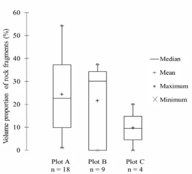
The volume proportions of rock fragments in plots A, B and C at the soil pit scale are presented in Figure 2. For plots A and B, the rock fragment contents were measured from soil sampling. For plot C, the rock fragment content was visually estimated. The volume content of rock fragments reached a maximum of 54 % for plot A, 35% for plot B and 20% for plot C. Mean values for the rock fragment contents were approximately 20 % for plots A and B and 10 % for plot C. These values exhibited significant dispersion, which suggests that there is a large degree of heterogeneity in the volume content of rock fragments.

Figure 2: Volume proportion of rock fragments in the three soil plots; n corresponds to the number of visual observations for plot C and the number of soil pits dug for plots A and B. The upper and lower box boundaries indicate the 75th and the 25th percentiles, respectively.

(10)

Catena, 92, 67‐74

Figure 3 (a, b, c) presents the apparent resistivity maps from the V1, V2 and V3 arrays for plot A. The resistivity values ranged between 5 and 130 ohm.m but showed a spatial organisation based on the soil depth (Fig. 3d). The apparent resistivity increased for thinner soils, i.e., when the bedrock was closer to the surface.

The interpreted resistivity map of the loamy-clay layer allowed the identification of two main areas of electrical resistivity (Fig. 3); the highest values of about 70 to 100 ohm.m were located in the southeast region of the plot, where the thickness of the loamy-clay layer was relatively small at close to 0.3 m depth.

(11)

Version postprint

Catena, 92, 67‐74 Author Man u scri p t

Figure 3: Spatial pattern of data recorded and calculated on plot A. -a-, -b-, -c- : Apparent electrical resistivity measurements for the V1, V2 and V3 arrays, respectively. -d- : Map of the loamy-clay layer thickness. -e- : Interpreted electrical resistivity for the loamy-clay layer. -f- : Map of the standard deviations of the electrical resistivity measurements for the V1 array. -g- : Map of the standard deviations of the interpreted electrical resistivity measurements.

4.2 Estimation of the rock fragment contents at the plot scale

Comparisons among the apparent resistivity map, the interpreted resistivity map (Fig. 3a and Fig. 3e) and the soil map (Fig. 1) enhanced the localisation of stony soils that exhibit the

(12)

Version postprint

Catena, 92, 67‐74

highest resistivity values. Standard deviation values for both the apparent and interpreted resistivity maps are shown in Figures 3f and 3g. These values ranged from 2 to 90 ohm.m and exhibited a similar spatial organisation, i.e., the highest values were located in the southeast region where the rock fragment content was the highest.

Figure 4: Relationships between the standard deviation of the electrical resistivity data and the measurements of the volume proportion of rock fragments determined on plot A.

Linear equations were fitted to the rock fragment content and electrical resistivity data (Fig. 4). For the apparent resistivity data, geoelectrical values were compared to the rock fragment contents at the 0 – 45 cm depth. This thickness corresponded to the layer investigated by the V1 array, which can be locally different, i.e., thicker or thinner, than the real loamy-clay layer thickness. For the interpreted resistivity data, geoelectrical values were compared to the rock fragment contents of the entire loamy-clay layer with a variable thickness from 0.2 to 0.9 m. Manus crit d’auteur / Author Man u scri p t

Table 2: Parameters of the linear equations describing the relationship between rock fragment contents and the electrical resistivity data on Plot A.

Equation n Slope Intercept R²

Volumetric rock fragments = f(mean values of Apparent resistivity) 18 0.79 - 8.44 0.77

Volumetric rock fragments = f(mean values of Interpreted resistivity) 18 0.60 - 0.08 0.70

Volumetric rock fragments = f(standard deviation values of Apparent resistivity) 12 1.28 13.68 0.85

Volumetric rock fragments = f(standard deviation values of Interpreted resistivity) 11 0.74 15.67 0.77

The results of the statistical regressions are summarised in Table 2. High and significant coefficients of determination (0.70 to 0.85) were observed for the four equations. These relationships are in agreement with visual descriptions presented on maps (Fig. 3) in which

(13)

Version postprint

Catena, 92, 67‐74

the stony areas corresponded to highly resistant zones. However, the highest coefficients of determination (0.85 and 0.77) were obtained when the standard deviation values were used instead of the mean values. Thus, these relationships between the rock fragment content and the interpreted or apparent resistivity appeared to be robust equations for calculating the volume percentage of rock fragments at the plot scale; the first equation (i.e. using interpreted resistivity data) provided an estimate of the volume content of rock fragments in the loamy-clay layer, whereas the other equation (i.e. using apparent resistivity data) provided an estimate of the volume content of rock fragments in the first layer measured by the V1 array. The latter equation using only the standard deviation of the apparent resistivity is the most robust and easiest relationship; this equation does not require an inversion or knowledge of the soil thickness. In the next section, the standard deviation of the apparent resistivity will be used.

IV. Discussion

4.1 Validation using the electrical resistivity noise

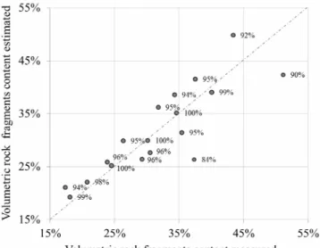
Geophysical surveys were conducted during the same period for plots A and B, and the data from plot B were used for the validation. Six of the nine pits dug on plot B were analysed because the remaining three pits were located in non-stony areas, and the rock fragment content would have been highly overestimated when using geoelectrical data. A significant correlation can be observed between the measured and estimated values for the volume content of rock fragments (Fig. 5) with a root mean square error of 5.4 % (Table 3) even though one point was underestimated by 10%.

p t Manus crit d’auteur / Author Man u scri p t

Figure 5: Comparison between the estimated and measured volume proportion of rock fragments. The percentage values represent the risk of rejection of the null hypothesis (“the difference between estimated and measured proportions is equal to 0”) when it is true.

(14)

Version postprint

Catena, 92, 67‐74

Table 3: Mean absolute errors (MAE), mean errors (ME) and root mean square errors (RMSE) for the estimations of the volume rock fragment content using i) the model using electrical resistivity noise and ii) the model of Bussian (1983). n is the number of soil pits used.

Plot A Plot B

Model using electrical resistivity noise

Model of Bussian (1983)

Model using electrical resistivity noise Model of Bussian (1983) n 12 12 6 6 MAE 0.03 0.05 4.01 0.02 ME -1.99E-06 0.04 -0.30 -0.01 RMSE 0.04 0.06 0.05 0.03

The map of the measured and estimated rock fragment contents is shown in Figure 6. The stony areas were correctly located. On plot A, some calculated values were overestimated by about 10% as compared to the measured values. However, this misestimation is considered to be reasonable and is probably not worse than that of a visual estimation in the field made by a pedologist. nuscrit d’auteur / Au th or Manuscri p t Manus crit d’auteur / Author Man u scri p t

Figure 6: Maps of the volume proportion of rock fragments for plots A and B as estimated by the noise electrical resistivity method. White areas correspond to no available data.

Thus, our methods appear to be useful for the estimation of rock fragment contents in stony soils.

(15)

Version postprint

Catena, 92, 67‐74

4.2 Calculation of the rock fragment content using the model of Bussian (1983)

The volume content of rock fragments on plots A and B was calculated by applying Eq. Eq. (1) and compared with the measured values; the estimation of error was less than 6% (Table 3). The low root mean square error of the estimation shows that the model of Bussian (1983) is well suited for the calculation of the volume content of rock fragments from electrical resistivity data, but a prior calibration of the cementation factor is required.

A comparison of the method using the electrical resistivity noise to the model of Bussian (1983) (Table 3) shows that both models are robust.

Ma nuscrit d’auteur / Au th or Manuscri p t Manus crit d’auteur / Author Man u scri p t

4.3 Effect of water content on the estimation of rock fragment content

The geophysical surveys of plots A, B and C performed for different water contents in the soil were compared (Fig. 7). The relationship between the standard deviation of the apparent electrical resistivity and the volume content of rock fragments varied with the seasons. In wet seasons, the rock fragment content was less sensitive to the standard deviation values due to their small range. The opposite effect on sensitivity was observed during dry periods.

Figure 7: Relationship between the standard deviation of the apparent electrical resistivity data and the volume content of rock fragments. The numerical value above each point represents the mean field water content in cm3_cm-3_{. Water content values for plot A and B were similar.}

For plot C, five geophysical surveys performed in April 2006, June 2006, August 2006, October 2006 and March 2007 were compared, and the soil at these times contained different water contents. Thus, the effect of the water content of the soil on the relationship between the rock fragment content and the standard deviation of the apparent electrical resistivity could be evaluated (Fig. 8). As expected, the standard deviation of the apparent electrical resistivity was significantly higher when the soil moisture was low. An analysis of variance demonstrated the predominant effect of soil moisture on the standard deviation of the apparent resistivity (Table 4).

(16)

Version postprint

Catena, 92, 67‐74 y = -2.03x + 65.78 R² = 0.84 0 10 20 30 40 0 10 20 30 40

Mean water content per soil unit (g/100g)

M ea n s ta nda rd de vi at ion of a pp ar en t r es is tiv ity p er s oil u nit ( ohm .m )

Calcaric Cambisol developed over grey limestone

Calcaric Cambisol developed over soft limestone

Calcaric Cambisol developed over beige cryoturbed limestone Haplic Calcisol developed over beige cryoturbed material at medium depth

Figure 8: Standard deviation values of the apparent electrical resistivity as a function of water content on plot C. Each symbol refers to soil units previously presented in figure 1.

based on both rock fragment and water contents.

Sources of variation Degrees of freedom Sum of square Mean Square F value Pr (>F)

Table 4: ANOVA for the standard deviations of the apparent resistivity

Rock fragment content 1 144.34 144.34 15.27 0.001**

Water content 1 731.90 731.90 77.42 9.75e-08***

Residuals 17 160.71 9.45

To estimate the pro tion of rock fragm n the soil relationships between the soil

volume content of rock fragments and the standard deviations of the apparent resistivities must be calibrated with regard to so

roc

ethod we have developed using electrical resistivity noise allows the qualitative a few hectares. Quantitative correlations between the volum

wer

por ents i , the

il moisture. Moreover, to more accurately determine the k fragment content of soil, geophysical surveys should be performed during dry periods when the range of the standard deviation of electrical resistivity data is expected to be at its highest.

V. Concluding remarks

The m

detection of stony areas on zones of

e percentage of rock fragments and the standard deviation values of electrical resistivity e shown to be as good as those of the model of Bussian (1983) for the estimation of the volume content of rock fragments. Nevertheless, the following recommendation must be considered. 1) To evaluate the signal noise, the unfiltered raw electrical data must be used; filtered data usually produced by commercial devices would allow the prediction of only the locations of stony areas and not the real volume percentage of rock fragments. 2) When the

(17)

Version postprint

Catena, 92, 67‐74

proportion of rock fragments is less than 15%, the estimation of the volume content of rock fragments by electrical resistivity becomes more uncertain because noise in the electrical resistivity signal is based on factors besides the presence of rock fragments. As an alternative, the model of Bussian (1983) can be used after a calibration of the cementation factor. 3) To use a relationship between the electrical resistivity data and rock fragment content, calibration data are needed on a plot with equivalent soil types and rock fragment lithologies. 4) The influence of the water content of the soil on the relationship between the electrical resistivity data and the volume content of rock fragments indicates that i) geoelectrical surveys should be performed in dry climate conditions and ii) the relationship with soil moisture should be calibrated.

VI. Appendix: Optimisation process

sistivity were collected within a 5 m radius focused on the sampling locations for me

3, cor

ences

AFNOR, 2009. Recueil de normes. Qualité des sols - Pédologie. Méthode O 11272: Détermination de la masse volumique apparente sèche.

nd bricks. Fragblast: International Journal for

surveying. Soil & illage Research 79 (2), 239-249.

Besson, A., Cousin, I., Bourennane, H., Nicoullaud, B., Pasquier, C., Richard, G., Dorigny, A., King, D., 2010. The

nd soil survey. In Bouma, J.,

of soils and surface

On plots A and B, mean values of electrical re around the given points; these points were

asurements of rock fragment content. The optimisation process was conducted on plot A in

two steps. First, ρFE was fixed at 20 ohm.m; ρRF, m and RFC were estimated by optimisation

with the following constraints: i) 0 < estimated RFC < 0.55, ii) 1.3 < m < 4 (Attia, 2005; Pape et al., 1999; Schon, 1996) and iii) 200 ohm. m < ρRF < 1000 ohm.m (Telford et al., 1976). The optimisation process was then performed to calculate the estimated RFC values by applying Eq. (2.1) within 100 iterations, a tolerance of 5 % and an accuracy of 0.000001

during 100 s. m and ρRF values were set to minimise the root mean square error of the

estimation of the volume content of rock fragments. ρRF exhibited a bimodal distribution with two peaks located at approximately 200 and 1000 ohm.m, and m varied between 1.5 and 4.

In the second step, the ρRF value was fixed at 200 ohm.m for a cryoturbed limestone

substrate and 1000 ohm.m for the other calcareous substrates. m was set equal to 2.6

responding to the median value of the m distribution in the first step. ρFE was unchanged

and set equal to 20 ohm.m. The optimisation process was performed again using these fixed values. Estimates of the RFC values were calculated by applying Eq. (2.1) on plot A and then on plot B.

Refer

s physiques. NF IS

Attia, A. M., 2005. Effects of petrophysical rock properties on tortuosity factor. Journal of Petroleum Science and Engineering

8, 185-198. 4

Bhattacharya, J., and Chandrakar, C., 1999. Comparison of three edge detection methods for image analysis of fragmented

andstones a s

Blasting and Fragmentation 3 (3), 251-265.

Besson, A., Cousin, I., Samouelian, A., Boizard, H., Richard, G., 2004. Structural heterogeneity of the soil tilled layer as

haracterized by 2D electrical resistivity c

T

spatial and temporal organization of soil water at the field scale as described by electrical resistivity measurements. European Journal of Soil Science 61 (1), 120-132.

ouma, J., 1985. Soil variability a B

and Nielsen, D.R. (eds). Soil spatial variability. Proc. Soil spatial variability workshop, Las Vegas, NV. 1984. PUDOC Wageningen, The Netherlands. pp 130-149.

Bourennane, H., King, D., Parco, R.L., Isambert, M., Tabbagh, . 1998. Three dimensional analysis

A

materials by electrical resistivity survey. European Journal of Environmental & Engineering Geophysics 3, 5-23.

(18)

Version postprint

Catena, 92, 67‐74

Bussian, A.E., 1983. Electrical conductance in a porous medium. Geophysics 48 (9), 1258-1268.

Cousin, I., Nicoullaud, B., Coutadeur, C., 2003. Influence of rock fragments on the water retention and water percolation in a calcareous soil. Catena 53 (2), 97-114.

Cousin, I., Besson, A., Bourennane, H., Pasquier, C., y measurements to the soil ydraulic functioning at the field scale. Comptes Rendus

, D., 2001. Multi-depth ontinuous electrical profiling for characterization of in-field

eoretical considerations for recision agriculture. In: Precision Agriculture (eds J. Stafford &

iafas, I., Chiarantini, L., 2011. Evaluation of the DIGISOIL

rnal of Sedimentary Petrology 21, 32-33. irard M-C. & Girard C-M., 1989 - Télédétection appliquée aux

imentale des propriétés électriques es roches. Potentiels d’électro filtration, suivi des mouvements

SS Working Group WRB. 2006. World reference base for soil 103. FAO, ome.

concentrates in the nge of 1.0 to 0.1 volume percent. American Mineralogist 70,

ship of the presence of a non-calcareous clay-loam orizon to DEM attributes in a gently sloping area. Geoderma

ranean environments (Coastal Cordillera of central hile). Earth Surface Processes and Landforms 32, 13-31.

39, 138-1144.

., Mary B., Coutadeur ., King D., 2004. Modélisation spatiale à l'échelle parcellaire

-161.

stigation: the ‘Vol-de-canards’ array. eophysical Prospecting 45 (6), 983-1002.

447-460.

ost, D.F., Martin, E.S.; Simanton, J.R., Sano, E.E., 1999. Use

litation 13 (2), 201-217.

with stony inclusions using eoelectrical measurements. Journal of Applied Geophysics 58

linity. Advances in Agronomy. 9: 201-251.

Research 83, 173-193.

eger, M., Cousin, I., Frison, A., Boizard, H., Richard, G., 2009.

103, 387-398.

. 346 pp.

il structure orizonation. Geoderma 97, 393-404.

nées et élimination des aleurs érronées en prospection électrique en continu. Revue

R.E., Keys, D.A., 1982. rospection géophysique. Propriétés électriques des roches,

magnétotellurique, rospection électromagnétique, eds ERG éditions La

B., Baize, D., Bouthier, A., Cousin, I., 011. The contribution of rock fragments to the available water Nicoullaud, B., King, D., Richard, G., 2009. From

spatial-continuous electrical resistivit h

Geoscience 341 (10-11), 859-867. Dabas, M., Tabbagh, A., Boisgontier c

variability. 3rd European Conference On Precision Agriculture. Montpellier, France.

Dabas, M. & Tabbagh, A., 2003. A comparison of EMI and DC methods used in soil mapping–th

p

A. Werner), Wageningen Academic Publishers, Muencheberg. pp. 121–129.

D

mapping tool with respect to the cost effectiveness. Report N° FP7-DIGISOIL-D4.3. 21 pp.

Folk L., 1951. A comparison chart for visual percentage estimation. Jou

G

zones tempérées et intertropicales, Masson, 260 pp. Guichet X., 2002. Etude expér

d

de fluides en zones hydrothermales. 211 pp. IU

resources 2006.

2nd edition. World Soil Resources Reports No. R

Jeffrey C. R., 1985. Comparison chart for estimating volume percentages of constituents in rocks and

ra 1318-1319.

King, D., Bourennane, H., Isambert, M., Macaire, J.J., 1999. Relation

h

89, 95-111.

Mathieu, R., Cervelle, B., Rémy, D., Pouget, M., 2007. Field-based and spectral indicators for soil erosion mapping in semi-arid mediter

C

Marescot L., 2006. Introduction à l’imagerie électrique du sous-sol. Bull. Soc. vaud. Sc. nat. 90.1: 23-40.

Michot, D., Benderitter, Y., Dorigny, A., Nicoullaud, B., King, D., Tabbagh, A., 2003. Spatial and temporal monitoring of soil water content with an irrigated corn crop cover using surface electrical resistivity tomography. Water Resources Research, 1

Nicoullaud B., Couturier A., Beaudoin N C

des effets de la variabilité des sols et des pratiques culturales sur la pollution nitrique agricole. In: Organisation spatiale des activités agricoles et processus environnementaux. P. Monestiez, S. Lardon, B. Seguin (eds). Coll. Science Update, INRA Editions, 143

Olhoeft, G.R., 1981. Electrical properties of rocks, in Physical Properties of Rocks and Minerals, eds Touloukian, Y.S., Judd, W.R. & Roy, R.F., McGraw Hill, New York. pp. 257–330. Panissod, C., Dabas, M., Jolivet, A., Tabbagh, A., 1997. A novel mobile multipole system (MUCEP) for shallow (0–3 m) geoelectrical inve

G

Pape, H., Clauser, C., Iffland, J., 1999. Permeability prediction based on fractal pore-space geometry. Geophysics 64, 1 1

Parkhomenko, E.I., 1967. Electrical Properties of Rocks, eds Plenum, New York. 314 pp.

P

of hand-held radiometers to evaluate the cover and hydrologic characteristics of semiarid rangelands. Arid Soil Research and Rehabi

Rey, E., Jongmans, D., Gotteland, P., Garambois, S. 2006. Characterisation of soils

g

(3): 188-201.

Rhoades, J.D., 1993. Electrical conductivity methods for measuring and mapping soil sa

4

Samouëlian, A., Cousin, I., Tabbagh, A., Bruand, A., Richard, G., 2005. Electrical resistivity survey in soil science: a review. Soil & Tillage

Schon, J.H., 1996. Physical Properties of Rocks: Fundamentals and Principles of Petrophysics. 600 pp.

S

Characterisation of the structural heterogeneity of the soil tilled layer by using in situ 2D and 3D electrical resistivity measurements. Soil & Tillage Research

Soil Survey Staff, 2010. Keys to Soil Taxonomy. In: U.S.D.A.-N.R.C. Service (Editor), Washington, DC

Sudduth, K.A., Drummond, S.T. & Kitchen, N.R., 2001. Accuracy issues in electromagnetic induction sensing of soil electrical conductivity for precision agriculture. Computers & Electronics in Agriculture 31, 239-264.

Tabbagh, A., Dabas, M., Hesse, A., Panissod, C., 2000. Soil resistivity: a non-invasive tool to map so

h

Tabbagh, A., 2004. Qwinv1De software. Tabbagh, J., 1988. Traitements des don v

d'Archéométrie 12, 1-9.

Telford W.M., Geldart, L.P., Sheriff, P

polarisation spontanée, tellurique, p

Barbannerie, Maurecourt. 221 pp. Tetegan, M., Nicoullaud, 2

content of stony soils: proposition of new pedotransfer functions. Geoderma 165, 40-49. crit d’auteur / Author Man u scri p t

(19)

Version postprint

Catena, 92, 67‐74

Ugolini, F.C., Corti, G., Agnelli, A., Certini, G., 1998. Under- and overestimation of soil properties in stony soils. 16th World Congress of Soil Science. Montpellier, France.