HAL Id: hal-03214660
https://hal.archives-ouvertes.fr/hal-03214660
Submitted on 3 May 2021
HAL is a multi-disciplinary open access
archive for the deposit and dissemination of
sci-entific research documents, whether they are
pub-lished or not. The documents may come from
teaching and research institutions in France or
abroad, or from public or private research centers.
L’archive ouverte pluridisciplinaire HAL, est
destinée au dépôt et à la diffusion de documents
scientifiques de niveau recherche, publiés ou non,
émanant des établissements d’enseignement et de
recherche français ou étrangers, des laboratoires
publics ou privés.
Distributed under a Creative Commons Attribution| 4.0 International License
Simulating the Earth system response to negative
emissions
C. Jones, P. Ciais, S. Davis, P. Friedlingstein, T Gasser, G Peters, J Rogelj, D
van Vuuren, J. Canadell, A Cowie, et al.
To cite this version:
C. Jones, P. Ciais, S. Davis, P. Friedlingstein, T Gasser, et al.. Simulating the Earth system response
to negative emissions. Environmental Research Letters, IOP Publishing, 2016, 11 (9), pp.095012.
�10.1088/1748-9326/11/9/095012�. �hal-03214660�
Simulating the Earth system response to negative
emissions
To cite this article: C D Jones et al 2016 Environ. Res. Lett. 11 095012
View the article online for updates and enhancements.
deployment in mitigation pathways: the case of water scarcity
Roland Séférian, Matthias Rocher, Céline Guivarch et al.
The effectiveness of net negative carbon dioxide emissions in reversing anthropogenic climate change
Katarzyna B Tokarska and Kirsten Zickfeld
-The role of large—scale BECCS in the pursuit of the 1.5°C target: an Earth system model perspective Helene Muri
-Recent citations
Quantifying Errors in Observationally Based Estimates of Ocean Carbon Sink Variability
Lucas Gloege et al
-Opportunities and challenges in using remaining carbon budgets to guide climate policy
H. Damon Matthews et al
-The role of prior assumptions in carbon budget calculations
Benjamin Sanderson
Environ. Res. Lett. 11(2016) 095012 doi:10.1088/1748-9326/11/9/095012
LETTER
Simulating the Earth system response to negative emissions
C D Jones1, P Ciais2, S J Davis3, P Friedlingstein4, T Gasser2,5, G P Peters6, J Rogelj7,8, D P van Vuuren9,10,
J G Canadell11, A Cowie12, R B Jackson13, M Jonas14, E Kriegler15, E Littleton16, J A Lowe1, J Milne17,
G Shrestha18, P Smith19, A Torvanger6and A Wiltshire1 1 Met Office Hadley Centre, FitzRoy Road, Exeter, EX1 3PB, UK
2 Laboratoire des Sciences du Climat et de l’Environnement, CEA CNRS UVSQ, Gif-sur-Yvette, France 3 Department of Earth System Science, University of California, Irvine, USA
4 College of Engineering, Mathematics and Physical Sciences, University of Exeter, Exeter EX4 4QE, UK
5 Centre International de Recherche en Environnement et Développement, CNRS-PontsParisTech-EHESS-AgroParisTech-CIRAD,
F-94736 Nogent-sur-Marne, France
6 Center for International Climate and Environmental Research—Oslo (CICERO), Gaustadalléen 21, NO-0349 Oslo, Norway 7 Energy Program, International Institute for Applied Systems Analysis, Schlossplatz 1, A-2361 Laxenburg, Austria
8 Institute for Atmospheric and Climate Science, ETH Zurich, Universitätstrasse 16, 8092 Zurich, Switzerland 9 PBL Netherlands Environmental Assessment Agency, The Netherlands
10 Copernicus Institute for Sustainable Development, Utrecht University, The Netherlands
11 Global Carbon Project, CSIRO Oceans and Atmosphere Research, GPO Box 3023, Canberra, Australian Capital Territory 2601, Australia 12 NSW Department of Primary Industries, University of New England, Armidale NSW 2351, Australia
13 Department of Earth System Science, Woods Institute for the Environment and Precourt Institute for Energy, Stanford University,
Stanford, CA 94305, USA
14 Advanced Systems Analysis Program, International Institute for Applied Systems Analysis, Schlossplatz 1, A-2361 Laxenburg, Austria 15 Potsdam Institute for Climate Impact Research(PIK), PO Box 60 12 03, D-14412 Potsdam, Germany
16 University of East Anglia, Norwich Research Park, Norwich NR4 7TJ, UK 17 Stanford University 473 Via Ortega, Stanford, CA 94305-2205, USA
18 US Carbon Cycle Science Program, US Global Change Research Program, Washington, DC 20006, USA
19 Institute of Biological and Environmental Sciences, University of Aberdeen, 23 St Machar Drive, Aberdeen, AB24 3UU, UK
E-mail:chris.d.jones@metoffice.gov.uk
Keywords: climate, carbon cycle, earth system, negative emissions, carbon dioxide removal, mitigation scenarios Supplementary material for this article is availableonline
Abstract
Natural carbon sinks currently absorb approximately half of the anthropogenic CO
2emitted by fossil
fuel burning, cement production and land-use change. However, this airborne fraction may change in
the future depending on the emissions scenario. An important issue in developing carbon budgets to
achieve climate stabilisation targets is the behaviour of natural carbon sinks, particularly under low
emissions mitigation scenarios as required to meet the goals of the Paris Agreement. A key requirement
for low carbon pathways is to quantify the effectiveness of negative emissions technologies which will be
strongly affected by carbon cycle feedbacks. Here we
find that Earth system models suggest significant
weakening, even potential reversal, of the ocean and land sinks under future low emission scenarios.
For the RCP2.6 concentration pathway, models project land and ocean sinks to weaken to 0.8±0.9
and 1.1±0.3 GtC yr
−1respectively for the second half of the 21st century and to
−0.4±0.4 and
0.1±0.2 GtC yr
−1respectively for the second half of the 23rd century. Weakening of natural carbon
sinks will hinder the effectiveness of negative emissions technologies and therefore increase their
required deployment to achieve a given climate stabilisation target. We introduce a new metric, the
perturbation airborne fraction, to measure and assess the effectiveness of negative emissions.
1. Introduction
In the recently adopted UN Paris Agreement on climate change, countries agreed to focus international
climate policy on keeping global mean temperature increase well below 2°C above pre-industrial levels and pursue actions to further limit warming to 1.5°C (UNFCCC 2015). Scenarios consistent with such
OPEN ACCESS
RECEIVED
24 March 2016
REVISED
26 August 2016
ACCEPTED FOR PUBLICATION
26 August 2016
PUBLISHED
20 September 2016
Original content from this work may be used under the terms of theCreative Commons Attribution 3.0
licence.
Any further distribution of this work must maintain attribution to the author(s) and the title of the work, journal citation and DOI.
targets typically require large amounts of carbon dioxide removal(Clarke et al2014, Gasser et al2015, Rogelj et al 2015), achieved by deliberate human
efforts to remove CO2from the atmosphere. Negative
emissions technologies(NETs) are therefore present in the majority of scenarios that give a more than 50% chance of limiting warming to below 2 °C (Fuss et al2014) and all scenarios that give more than a 50%
chance of staying below 1.5°C (Rogelj et al2015).
In low emission pathways, the presence of NETs offsets continued positive emissions from fossil fuels and land-use change to strongly reduce the anthro-pogenic input into the atmosphere. In some cases it even reverses the sign so that the effect of human activ-ity is a netflow out of the atmosphere (‘net negative emissions’). Gasser et al (2015) stress the need to
sepa-rately quantify the magnitude of continued positive emissions and the amount of carbon removed by negative emission technologies.
Fuss et al (2014) called for renewed efforts to
develop a consistent and comprehensive narrative around NETs and the need to develop a framework for examining implications of NETs in a wider context. Smith et al(2016) reviewed costs and biophysical limits
associated with different NET technologies. Research into NETs needs to address both demand-side(how much NETs are required?) and supply-side (how much NETs are possible?) questions. This paper specifically explores the Earth system responses to different amounts of negative emissions. Understanding of the behaviour of natural carbon sinks is crucial to quantify the demand for NETs to achieve climate targets.
Although the natural carbon cycle is now com-monly represented in Earth system models(ESMs), there has been little specific analysis of the behavior of different components of the carbon cycle when forced by net negative emissions. Previous analysis of CMIP5 ESMs has shown that approximately half of the models require globally net negative emissions for CO2to
fol-low the RCP2.6 pathway(Jones et al2013). Tokarska
and Zickfeld (2015) used an ESM of intermediate
complexity to simulate the response to a range of future NET scenarios. It is known that redistribution across natural carbon stocks weakens the effect of negative emissions on atmospheric CO2(see e.g. Cao
and Caldeira2010, Matthews2010, Ciais et al2013, MacDougall2013). Reducing the amount of CO2 in
the atmosphere reduces the natural carbon sinks due to the fact that vegetation productivity will decrease when CO2decreases and that ocean CO2uptake will
also decrease with decreasing CO2.
In this paper, we assess the impact on the global carbon cycle across different time horizons and con-sider different balances of emissions andfluxes, and how the natural carbon cycle responds. For this, we use, for thefirst time, CMIP5 model simulations to quantify how the Earth system may respond to NETs, and how this response may depend on the state of the climate and the background scenario.
We stress the need to know quantitatively what happens to this redistribution of carbon under specific scenarios in order to both plan the requirement for NETs, and to understand their effectiveness and any implications or side effects. Despite the fact that they lack some important processes such as permafrost car-bon, process-based and spatially explicit ESMs remain an essential tool for this exploration. Reducing uncer-tainty in projected carbon sinks behaviour, especially under low emissions scenarios, is a pressing research priority.
Section2of this paper draws on existing CMIP5 ESM simulations of the RCP2.6 scenario, extended to 2300 with sustained global negative emissions, and section3makes use of a simple climate-carbon cycle model to explore the scenario dependence of the response of carbon sinks to negative emissions.
2. Earth system response over time
The contemporary carbon cycle can be summarised at a global scale: human activity puts CO2 into the
atmosphere, natural sinks remove about half of those emissions and the remainder accumulates in the atmosphere such that atmospheric CO2
concentra-tions increase (figure 1). Since pre-industrial times,
human activity has always resulted in net positive emissions to the atmosphere, leading to an increase of atmospheric CO2 concentration, from about 288 to
400 ppm over the last 150 years or so. Natural ecosystems, both land and oceans, have been persis-tent sinks of CO2(Le Quéré et al2015).We will build
onfigure1throughout this paper to depict schemati-cally how the carbon cycle responds to carbon dioxide removal.
Different types of anthropogenic activity have dif-ferent effects on the Earth system and carbon pools. Figure2shows schematically how each pool is affected by direct anthropogenic activity and subsequent redis-tribution between pools. We restrict consideration here to those carbon pools which respond on time-scales up to a few centuries. By this we mean the atmosphere; the land vegetation and near surface(top metre or so) soil organic matter but not deep perma-frost or geologically stored carbon; and the ocean store of dissolved(organic or inorganic) carbon and bio-mass in various forms of plankton, but not ocean sediments.
Land-use change, mainly in the form of deforesta-tion, was thefirst major human perturbation to the carbon cycle(Le Quéré et al2015). Its net result was to
move carbon from the land pool(L) to the atmosphere (A) (shown in figure2(a)). Over time, natural sinks
redistributed part of this additional carbon in the atmosphere between the other pools. Atmospheric CO2(A) increases, but the total mass of carbon (A+L
Since about 1950, the burning of fossil fuel repre-sents a larger source of CO2to the atmosphere than
land-use change and this has a different effect on the carbon cycle(figure2(b)) because carbon originating
from a separate reservoir is introduced,firstly to the atmosphere and subsequently partly redistributed between the land and ocean. A major difference from land-use emissions is that the total amount of carbon in the atmosphere-land-ocean system increases. This is depicted infigure2by an increased size of the pie chart in row b relative to the original size, shown by the dotted circle.
Figure2then shows two possible ways of obtaining carbon-neutral energy. Thefirst is through use of bioe-nergy(figure2(c)) whereby carbon is first drawn down
from the atmosphere by vegetation growth and stored in biomass(arrow ‘1’ in figure2(c)) before this biomass
is burned to release energy, releasing the stored carbon back to the atmosphere(arrow ‘2’ in figure2(c)). We
note that the drawdown of carbon into vegetation may have occurred many years prior to the burning of the fuel, and so the concept of bioenergy being carbon neu-tral is not necessarily true on short timescales (Cher-ubini et al2011). The fourth row in figure2then shows how fossil fuel can be burned, but can be brought to being approximately carbon neutral by using carbon capture and storage technology(CCS). In reality not all the carbon will be captured (IPCC 2005, Benson et al2012), and some may escape during the capture,
transport and ultimate storage processes, but con-ceptually thefigure captures the intention of CCS to enable low-carbon fossil fuel use.
Now we consider the role of NETs. If CO2 is
removed from the atmosphere and stored in land vegetation and soils (e.g. by afforestation) then the
total amount of carbon(A+L+O) does not change and in the context of thisfigure, this is just a form of land-use change. However, if the NET employed stores the carbon in a geological formation(or deep ocean or inert soil pool), as depicted in figure 2(e),
then the size of the active carbon cycle is reduced (smaller pie chart in row e). The figure shows two spe-cific activities: bioenergy with carbon capture and sto-rage(BECCS) removes carbon from the atmosphere via the land(arrows 1 and 2) whereas direct air capture removes it directly from the atmosphere. Other NETs could also be depicted in a similar way but we show just two here for clarity. In the same way that additions to the atmosphere lead to redistributions of carbon to land and ocean, removal from the atmosphere also leads to redistribution between the three pools(Cao and Caldeira2010).
2.1. Research questions
All these anthropogenic activities have substantially different effects on the Earth system, but one common theme (except for CCS in an idealised case) is the redistribution of carbon between reservoirs, which continues for some time after the initial activity. For all actions depicted infigure2, the long-term response(in the right hand columns) differs from the immediate effect shown in the left-hand column. In order to understand the impact of any action we need to quantitatively understand how this redistribution will operate at the process level. The natural carbon sinks that drive this redistribution are affected by the prevailing climate and CO2 concentration and also
historical changes in their environmental conditions. In scenarios where CO2 growth slows and CO2
concentration either stabilizes, or even peaks and
Figure 1. Summary of changes in the global carbon budget since 1870.(Redrawn based onhttp://folk.uio.no/roberan/img/ GCP2015/PNG/s15_Waterfall_sources_and_sinks.png). Atmospheric CO2concentration has changed from about 288 ppm in 1870
to 397 in 2014 due to emissions from fossil fuel burning and land-use change and natural sinks on land and ocean. For consistency with later analysis we introduce a bar to thisfigure to represent NETs, but its magnitude over this period has been zero. For full details of the global carbon budget see Le Quéré et al(2015).
3
declines, then natural sinks may behave rather differ-ently than currdiffer-ently where concentration is always on the rise. The airborne fraction of emissions(AF) has been approximately constant for many decades now but this is not a fundamental behaviour of the Earth system, but largely a result of near-exponential growth in carbon emissions (Raupach 2013, Raupach et al2014). AF may change markedly in the next
cen-tury dependent on the scenario of anthropogenic emissions. Jones et al(2013) showed strong changes in
the land and ocean uptake fraction for the 21st century compared with the 20th century. Beyond 2100, we may expect further changes and qualitatively different behaviour of the land and ocean sinks.
Long simulations using ESMs provide a quantita-tive understanding of the multiple trade offs and com-peting factors within the Earth system. Here we explore a case study of RCP2.6(van Vuuren et al2011)
using simulations from CMIP5 ESMs. This scenario is the only high mitigation scenario that has been
Figure 2. Schematic representation of how the carbon cycle system responds to anthropogenic activity. Each row depicts the initial action and the subsequent response of the system in terms of distribution of carbon between three pools: atmosphere(A), land (L) and ocean(O). As explained in the text, we do not include pools that only respond on very long timescales such as geological carbon or ocean sediments. The sizes of the three pools are not to scale(for example the ocean carbon pool is much bigger than the other two). Thefive rows depict different anthropogenic activities in an approximate chronological sequence as discussed in the text: (a) land use change;(b) fossil fuel burning; (c) bioenergy (without carbon capture); (d) carbon capture and storage (CCS) applied to fossil fuel burning;(e) negative emission technologies (NETs) with BECCS and DAC shown as examples and described in the text. In rows (b) and(e) the dotted circle on the right-hand pie chart denotes the original size of the pie chart from the left hand side.
simulated by multiple ESMs—it shows emissions peaking at just over 10 GtC yr−1in 2020, then declin-ing, becoming net negative during the 2080s. The reduction in global emissions is driven partly by reduced fossil fuel use and partly by the introduction of BECCS as early as 2020. The total NETs deployed during the 21st century is much bigger than the amount of global net negative emissions after 2080. An extension to the scenario exists which assumes con-stant emissions(of −0.42 GtC yr−1) from 2100 until 2300(Meinshausen et al2011).
Here we look at the available CMIP5 models (table1) which extended their simulations up to 2300.
A fifth model, BCC-CSM1.1, also performed this simulation, but without land-use change as a forcing of the land carbon cycle meaning that its land carbon response is therefore very different from the other models(see figure 2(a) of Jones et al2013) and so we
do not include it here. 2.2. Results
In this section we present the results following a narrative beginning with anthropogenic emissions and leading through to the simulated land and ocean sinks and their resulting effect on atmospheric CO2.
The methods section of the supplementary informa-tion explains how we derive these results from the CMIP5 concentration-driven simulations and how we construct thefigures shown here. We start by showing the RCP2.6 CO2pathway and the simulated land and
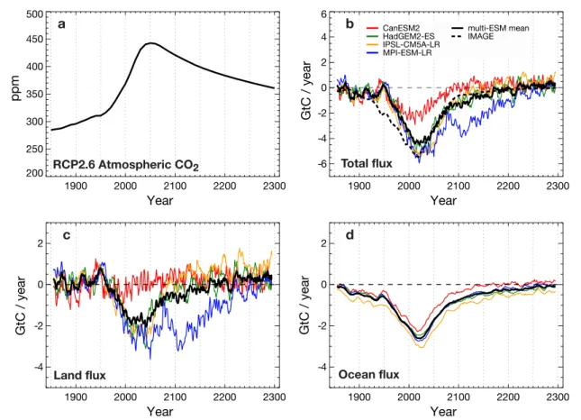
ocean carbon fluxes by the 4 ESMs as well as the IMAGE integrated assessment model which generated the RCP2.6 scenario(figure3).
The emissions, CO2concentration and simulated
response of land and ocean sinks are detailed in table S1. The behaviour of the simulated carbon sinks is as expected from figure 1; as anthropogenic emissions increase(not shown), natural sinks increase to absorb approximately half of this, and therefore atmospheric CO2increases. For comparison, the MAGICC
calcula-tions (Meinshausen et al2011) have been added in
figure3(b), showing consistent results. This provides
confidence that IAM calculations (using MAGICC) are able to simulate similar dynamics over time to the current state-of-the-art descriptions of the carbon cycle in ESMs.
During the 21st century, anthropogenic NETs along with other mitigation activities come into play in the scenario and gradually reduce and eventually reverse anthropogenic total input from strong positive emissions to weak positive and then a global negative emission. The land and ocean sinks do not respond to the instantaneous emission rate but to the history of the land and ocean carbon reservoirs and level of atmospheric CO2 and climate change above
pre-industrial levels. To illustrate this clearly we analyze the simulations in 50 year sections and calculate the multi-model mean response. Figure4shows quantita-tively the balance between the various components as they evolve in time:
• 2000–2050. The application of NETs begins but anthropogenic activity remains dominated by posi-tive emissions(figure4(a)). Land and ocean sinks
persist. The AF remains close to half of emissions and CO2concentration continues to rise.
• 2050–2100. Fossil fuel emissions decline and NETs grow further in this scenario. The anthropogenic total is still positive but much smaller(figure4(b)).
Natural sinks persist—a little reduced but still absorbing carbon due to past history and therefore CO2begins to decrease, despite the anthropogenic
total still being positive.
• 2100–2150. NETs exceed fossil inputs and human activity removes more CO2than it emits at a global
scale (figure 4(c)). During this first 50 years of
anthropogenic net carbon removal, the natural sinks weaken significantly due to the rapid decrease in atmospheric CO2. Hence there is an atmospheric
CO2 reduction due to the combination of net
negative anthropogenic emissions and land and ocean still absorbing carbon, however not as strong as might have been expected if strong natural sinks had persisted.
• 2150–2200 and on to 2250. Behaviour is qualita-tively similar tofigure4(c), but now natural sinks
have weakened further and CO2decrease is slowed.
Towards 2250 natural sinks are all but gone. In fact 3 out of 4 ESMs simulate a reversal of the land carbon sink to become a source.
• 2250–2300. In the final stage the land and ocean system has become a net source of CO2. Most ESMs
still simulate the ocean as a sink, but the overall (land plus ocean) flux is positive (figure4(d)). The
atmospheric CO2 decrease is weakened as the
natural carbon cycle is releasing carbon to the atmosphere, working in the opposite direction to the anthropogenic removal via NETs.
In summary, these results show a clear succession of events: from 2000 to 2050 the emergence of NETs has a slowing effect on anthropogenic emission but the
Table 1. List of models and modelling centres contributing to CMIP5 whose data has been used for this analysis. In terms of their climate and carbon cycle response under RCP2.6, these models represent a reasonable span of model spread from the CMIP5 ensemble(see the supplementary information or for example figure 6(b) of Jones et al2013).
Modelling centre Model name Canadian Centre for Climate modelling and
analysis(CCCma)
CanESM2 Met Office Hadley Centre (MOHC) HadGEM2-ES Institut Pierre-Simon Laplace(IPSL) IPSL-CM5A-LR Max Planck Institute for Meteorology(MPI-M) MPI-ESM-LR
5
general balance is not changed from the historical per-iod; from 2050 to 2100 natural sinks outweigh(still positive) anthropogenic emissions and CO2begins to
fall; from 2100 to 2250 NETs exceed fossil emissions and human activity is a global negative emission; finally, from 2250 to 2300 natural sinks saturate and reverse and oppose any further removal.
3. State and scenario dependence of the
Earth system response
We know that natural carbon sinks and the AF of emissions are sensitive to climate change and behave differently under different future scenarios. It is there-fore important to understand how the effectiveness of NETs may also differ depending on the scenario against which they are applied. In this section we look at the range of Earth system responses to different levels of negative emissions when applied under different climate and CO2scenarios.
To this end we perform new simulations as pertur-bations to the RCP set of projections. Using the Hadley Centre Simple Climate-Carbon Model widely used in previous studies (Jones et al 2003, 2006, House et al2008, Huntingford et al2009—see SI for more
details) we quantify the effect of the level of past
emissions and climate change on the effectiveness of different levels of NETs.
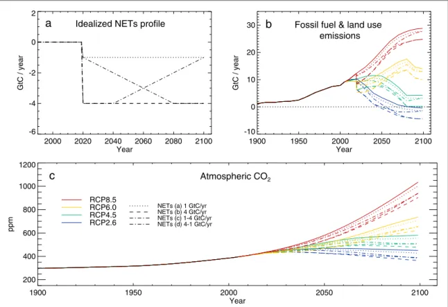
We take each of the four RCP emissions scenarios as a baseline and apply on top of them four idealised scenarios of additional negative emissions (figure 5(a)). The negative emissions scenarios we
impose all begin in 2020 and comprise: (a) Constant removal of 1 GtC yr−1.
(b) Constant removal of 4 GtC yr−1.
(c) A linear increase in removal from 1 GtC yr−1in
2020 up to 4 GtC yr−1 in 2080 followed by sustained 4 GtC yr−1removal until 2100.
(d) The same as (c) but reversed in time to remove 4 GtC yr−1from 2020 to 2040 and then gradually reduce the removal rate to 1 GtC yr−1by 2100. The total CO2removal for the 2020–2100 period
under these idealised scenarios is 80 and 320 GtC under thefirst two and 230 GtC for the last two. The idealised NET profiles are added to the four RCP emis-sions scenarios(figure5(b)). The simple model is run
in emissions-driven configuration taking these emis-sions as input and simulating the response of natural
Figure 3. RCP2.6 scenario and CMIP5 simulated carbonfluxes. (a) RCP2.6 CO2concentration pathway;(b) total (land plus ocean)
carbonflux from CMIP5 ESMs; (c) and (d) land and ocean fluxes separately. Four CMIP5 ESMs were used (listed in table1) and results are shown as 10 year smoothedfluxes. The black line shows the multi-ESM mean and the dashed black line in (b) shows the MAGICC results for the RCP2.6 scenario(used by the IMAGE IAM in creating RCP2.6). The sign convention is to plot the land and ocean as positive for aflux to the atmosphere and negative to represent a sink. Vertical dotted lines show 50 year time periods used to aggregate results discussed in the text.
sinks and atmospheric CO2 concentration
(figure5(c)). Here we explore the effect of the applied
negative emission and to what extent the Earth-system response depends on the magnitude or time profile of the NET or the state or scenario of background climate and CO2.
Figure 5(c) shows the obvious result that with
additional NETs applied to each scenario, the simu-lated CO2is reduced. But the degree of reduction
var-ies significantly between scenarios. For example, the same 320 GtC removal results in reduced atmospheric CO2 by 178, 211, 237 and 274 GtC for RCP2.6 to
RCP8.5 respectively. It is clear that the effectiveness of negative emissions varies depending on the scenario and the state of the Earth system. It is therefore desir-able to define a new metric that can measure this dependence.
The AF is a commonly used metric and we adopt it here to allow afirst analysis of the results. It can be defined as an instantaneous value as the ratio of a sin-gle year rise in CO2divided by that year’s emissions, or
a long-term cumulative quantity defined as the change over many years of CO2 divided by the cumulative
emissions over that period. When considering either
emissions close to zero or CO2 changes that can
change sign, then the former definition is not always well behaved or well defined, and so we adopt the latter definition (hereafter named the cumulative airborne fraction, CAF).
Table2shows the cumulative emissions and their impact on atmospheric CO2for the scenarios with and
without added negative emissions over the 80 year per-iod from 2020–2099. The table shows the CAF for the un-modified RCP scenarios, and then also for each modified scenario. A detailed derivation of the terms shown in table 2 is given in the supplementary information.
The CAF of the original RCP scenarios varies markedly across RCPs, with RCP2.6 having a small fraction of cumulative emissions remaining in the atmosphere for the 2020–2099 period (only 15%) while the other RCPs have a higher fraction of cumula-tive emissions remaining in the atmosphere, ranging from 48% for RCP4.5 to 72% for RCP8.5(column 7 in table2, and see SI text andfigure S3). This is consistent with previous studies (Ciais et al 2013, Jones et al2013). When we look at the CAF under the
mod-ified scenarios (column 8) we find two things. For
Figure 4. The four stages of succession of the differing balance betweenflux components. As for figure1the bars show changes in atmospheric CO2(ppm) due to that emission or flux. Each panel shows a selected 50 year period from the RCP2.6 simulations to
analyze the changing balance of theflux components. Due to small differences between the compatible emissions diagnosed from the four ESMs and the emissions in the scenario each 50 year period does not balance precisely(see SI for details).
7
RCP2.6 the values vary hugely between the three addi-tional NET scenarios (figure S3e). This is because either or both the cumulative emissions or the change in atmospheric CO2 are negative and this leads to
changes in sign of CAF and values greater than one because the denominator in the definition is small. For RCP6 and RCP8.5(and to some extent for RCP4.5) we find an opposite result—the CAF is rather insensitive to the CO2removal and stays close to the value from
the un-modified scenario. In either case this metric therefore is not very useful as a measure of either the effect of the negative emission on the Earth system or of the Earth system on the negative emission.
We also calculate the fraction of the CO2removal
which has remained out of the atmosphere—i.e. the AF of the negative emission(final column of table2; figure S3 panels m–p). For each RCP this metric is rather insensitive to the amount of removal and is dif-ferent from(and generally bigger than) the CAF of the RCP itself for the same period. This means that the effect of NETs on atmospheric CO2in the long term is
more closely controlled by the background scenario and level of climate change than by the amount of NETs themselves. Comparing the ramped removals with different time profiles of the same cumulative amount we see that the response is not strongly affec-ted by the removal pathway. Tokarska and Zickfeld (2015) also calculated a CAF of their carbon removal
and found it to be less dependent on the amount of removal than a CAF based on total emissions. Here we have shown that this property applies across the full range of RCP scenarios. We argue that this perturba-tion AF(PAF) is therefore a more suitable metric to assess the efficiency of NET than the CAF of the emis-sions from a single simulation.
This result has several significant implications. Firstly, that it is meaningful to define an AF of a per-turbed emission on top of a background scenario in order to measure the effect on atmospheric CO2of the
additional emission or removal. Secondly, this PAF is not the same as the AF of the background scenario itself. Hence, if it is desired to calculate the effect of adding or removing an amount of carbon on top of an existing scenario, then knowing the AF of the scenario does not help—one must calculate the AF of the extra carbon removed instead, i.e. the PAF. Thirdly, though, the PAF from a given scenario is rather insensitive to the magni-tude and timing of additional emission. This may be expected when the additional emission is a small frac-tion of the total emitted carbon for the scenario, but it appears to hold here too even for RCP2.6 when the total carbon removal is bigger than the cumulative emission in the underlying scenario. This means that once a PAF has been calculated relative to a scenario it can be approximately applied to other perturbations about that scenario to estimate their eventual impact.
Figure 5. Simulated CO2concentration under four RCP emissions scenarios with added idealised profiles of CO2removal from NETs.
The top panels show the inputs to the model:(a) the idealised NET profiles and (b) the total anthropogenic emissions when these NETs are added to the RCP emissions scenarios. RCP emissions(solid lines) with the idealised NETs added (dashed lines). The bottom panel(c) shows the resulting atmospheric CO2simulated by the simple carbon cycle model.
Table 2. Cumulative emissions and changes in atmospheric CO2for the simple model simulations of the original and modified RCPs with additional NET scenarios added. The cumulative airborne fraction (CAF) is calculated for the scenarios and also just for the NET components as described in the text.*The definition and calculation of these metrics is explained in more detail in the SI.
RCP scenario Idealised NET profile/GtC yr−1 RCP cumulative emis-sion(2020–2099)/GtC Cumulative addi-tional NE/GtC
Cumulative total emis-sion(2020–2099)/GtC
Change in atmo-spheric CO2/GtC
CAF of back-ground RCP*(2020–2099)
CAF of modified RCP* with NET(2020–2099)
Perturbation-AF of the additional negative
emis-sion* RCP2.6 243 37 0.15 −1 −80 163 −10 −0.06 0.6 −4 −320 −77 −141 1.83 0.57 −1 to −4 −230 13 −101 −7.8 0.6 −4 to −1 −230 13 −86 −6.6 0.55 RCP 4.5 663 316 0.48 −1 −80 583 261 0.45 0.7 −4 −320 343 105 0.3 0.67 −1 to −4 −230 433 155 0.35 0.7 −4 to −1 −230 433 169 0.39 0.66 RCP 6.0 1060 649 0.61 −1 −80 980 588 0.6 0.78 −4 −320 740 412 0.55 0.75 −1 to −4 −230 830 470 0.56 0.78 −4 to −1 −230 830 483 0.58 0.74 RCP 8.5 1764 1265 0.72 −1 −80 1684 1195 0.71 0.89 −4 −320 1444 991 0.68 0.87 −1 to −4 −230 1534 1061 0.69 0.89 −4 to −1 −230 1534 1071 0.70 0.86 9 Environ. Res. Lett. 11 (2016 ) 095012
4. Conclusions
Other studies have outlined various socio-economic costs, biophysical limits and implications of different NETs (Fuss et al 2014, Smith et al 2016, William-son2016). Here we have shown how NETs interact
with the physical climate-carbon cycle system. Our analysis of the Earth system response to negative emissions has provided new insights and identified future research priorities.
Our results contribute to the need to quantify the interactions between the climate, carbon cycle and anthropogenic NETs in determining future redis-tribution of carbon between atmosphere, land and ocean reservoirs. By viewing the scenarios and the evolution of carbon sinks and sources in a sequence of phases we have revealed qualitatively different beha-viour of the Earth system at different points in time. The combined effect of anthropogenic and natural sources and sinks can change over time, sometimes resulting in positive and sometimes negative changes in atmospheric CO2concentration. The behavior of
atmospheric CO2is not predictable from the
instanta-neous anthropogenic emission alone, but requires knowledge of past emissions and Earth system state. For example, CMIP5 simulations following the RCP2.6 pathway to 2300 exhibited periods where atmospheric CO2decreased despite ongoing net
posi-tive emissions from anthropogenic activity. Con-versely, later in the scenarios, natural sinks weakened and even reversed, especially on land, and offset the effects of globally negative anthropogenic emissions.
We found significant state-dependence of the Earth system behaviour in response to NETs. Our results showed that the effect of NETs on atmospheric CO2is more closely controlled by the background
sce-nario and level of climate change than by the amount or timing of NETs themselves. We propose a new metric, the PAF, defined as the ratio of CO2reduction
to the amount of NETs applied. This metric can be used to transfer model results that quantify the effect of NETs under a given scenario to estimate the effect of different levels of NETs against the same scenario.
Simplified climate-carbon cycle models, calibrated against complex ESMs and often used in IAMs for sce-nario generation are capable of reproducing this beha-viour at a global scale. This means that existing IAMs are not systematically wrong in their estimates of NETs required within scenarios. However, large uncertainty remains, due primarily to model spread in the simula-tion of future carbon sinks and this hinders robust deter-mination of carbon budgets to meet climate targets.
ESMs still lack some important processes such as the role of nutrient cycles that may limit future land car-bon storage(Zaehle et al2015), burning of old land
car-bon stocks (e.g. peat fires in Indonesia, Lestari et al2014) or release of carbon from thawing
perma-frost(Schuur et al2015). The latter in particular has
potentially significant impacts on the requirement for
negative emissions, as once released from thawed per-mafrost it would take centuries to millennia for the same carbon to re-accumulate, making it effectively irreversible on human timescales (MacDougal et al2015). Uncertainty also exists on the strength and
persistence of concentration-dependent carbon uptake, especially on land(so-called ‘CO2fertilisation’). IPCC
5th Assessment Report assessed‘low confidence on the magnitude of future land carbon changes’ (Ciais et al2013). It is increasingly important to bring
observa-tional constraints to bear to reduce this uncertainty especially focusing on low emissions scenarios.
It is increasingly clear that negative emissions could be very important in achieving ambitious cli-mate targets, and in fact many scenarios rely on them to do so. Failure to accurately account for carbon cycle feedbacks which increase the need for such negative emissions may strongly and adversely affect the feasi-bility of achieving these targets. We lack important understanding about the costs and implications of negative emissions, and also knowledge related to the Earth-system dynamics. It is vital to address these knowledge gaps in order to quantify the requirement for, and implications of negative emissions.
Acknowledgments
The work of CDJ, JAL and AW was supported by the Joint UK BEIS/Defra Met Office Hadley Centre Climate Programme(GA01101). CDJ, JAL, AW, PF, EK and DvV are supported by the European Union’s Horizon 2020 research and innovation programme under grant agreement No 641816 (CRESCENDO). GPP was supported by the Norwegian Research Coun-cil(project 209701). PC acknowledges support from the European Research Council Synergy grant ERC-2013-SyG-610028 IMBALANCE-P. We acknowledge the World Climate Research Programme’s Working Group on Coupled Modelling, which is responsible for CMIP, and we thank the climate modeling groups(listed in table 1 of this paper) for producing and making
available their model output. For CMIP the US Depart-ment of Energy’s Program for Climate Model Diagnosis and Intercomparison provides coordinating support and led development of software infrastructure in partnership with the Global Organisation for Earth system Science Portals.
References
Benson S M et al 2012 Global Energy Assessment Toward a Sustainable Future(Cambridge: Cambridge University Press) ch 13
Cao L and Caldeira K 2010 Atmospheric carbon dioxide removal: long-term consequences and commitment Environ. Res. Lett. 5 024011
Cherubini F, Peters G P, Bernsten T, Stromman A H and Hertwich E 2011 CO2emissions from biomass combustion for
bioenergy: atmospheric decay and contribution to global warming GCB Bioenergy3 413–26
Ciais P et al 2013 Carbon and other biogeochemical cycles Climate Change 2013: The Physical Science Basis. Contribution of Working Group I to the Fifth Assessment Report of the Intergovernmental Panel on Climate Change ed T F Stocker et al(Cambridge: Cambridge University Press)
Clarke L et al 2014 Assessing transformation pathways Climate Change 2014: Mitigation of Climate Change. Contribution of Working Group III to the Fifth Assessment Report of the Intergovernmental Panel on Climate Change ed O Edenhofer et al(Cambridge: Cambridge University Press)
Fuss S et al 2014 Betting on negative emissions Nat. Clim. Change4 850–3
Gasser T, Guivarch C, Tachiiri K, Jones C D and Ciais P 2015 Negative emissions physically needed to keep global warming below 2°C Nat. Commun.6 7958
House J, Huntingford C, Knorr W, Cornell S E, Cox P M, Harris G R, Jones C D, Lowe J A and Prentice C I 2008 What do recent advances in quantifying climate and carbon cycle uncertainties mean for climate policy? Environ. Res. Lett.3 044002
Huntingford C, Lowe J A, Booth B B B, Jones C D, Harris G R, Gohar L K and Meir P 2009 Contributions of carbon cycle uncertainty to future climate projection spread Tellus61B 355–60
IPCC 2005 IPCC Special Report on Carbon Dioxide Capture and Storage. Working Group III of the Intergovernmental Panel on Climate Change ed B Metz et al(Cambridge: IPCC) pp 1–431 Jones C D et al 2013 Twenty-first-century compatible CO2
emissions and airborne fraction simulated by CMIP5 Earth system models under four representative concentration pathways J. Clim.26 4398–413
Jones C D, Cox P M and Huntingford C 2003 Uncertainty in climate-carbon cycle projections associated with the sensitivity of soil respiration to temperature Tellus55B 642–8 Jones C D, Cox P M and Huntingford C 2006 Climate-carbon cycle
feedbacks under stabilization: uncertainty and observational constraints Tellus58B 603–13
Lestari R K, Watanabe M, Imada Y, Shiogama H, Field R D, Takemura T and Kimoto M 2014 Increasing potential of biomass burning over Sumatra, Indonesia induced by anthropogenic tropical warming Environ. Res. Lett.9 104010
Le Quéré C et al 2015 Global carbon budget 2015 Earth Syst. Sci. Data7 349–96
MacDougal A H 2013 Reversing climate warming by artificial atmospheric carbon-dioxide removal: can a Holocene-like climate be restored? Geophys. Res. Lett.40 5480–5 MacDougal A H, Zickfeld K, Knutti R and Matthews H D 2015
Sensitivity of carbon budgets to permafrost carbon feedbacks and non-CO2forcings Environ. Res. Lett.10 125003
Matthews H D 2010 Can carbon cycle geoengineering be a useful complement to ambitious climate mitigation? Carbon Manage.1 135–44
Meinshausen M et al 2011 The RCP greenhouse gas concentrations and their extension from 1765 to 2300 Clim. Change109 213–41
Raupach M R 2013 The exponential eigenmodes of the carbon-climate system, and their implications for ratios of responses to forcings Earth Syst. Dynam.4 31–49
Raupach M R, Gloor M, Sarmiento J L, Canadell J G, Frölicher T L, Gasser T, Houghton R A, Le Quéré C and Trudinger C M 2014 The declining uptake rate of atmospheric CO2by land
and ocean sinks Biogeosciences11 3453–75 Rogelj J, Luderer G, Pietzcker R C, Kriegler E, Schaeffer M,
Krey V and Riahi K 2015 Energy system transformations for limiting end-of-century warming to below 1.5°C Nature Clim. Change5 519–27
Schuur E A G et al 2015 Climate change and the permafrost carbon feedback Nature520 171–9
Smith P et al 2016 Biophysical and economic limits to negative CO2
emissions Nat. Clim. Change6 42–50
Tokarska K B and Zickfeld K 2015 The effectiveness of net negative carbon dioxide emissions in reversing anthropogenic climate change Environ. Res. Lett.10 094013
UNFCCC 2015 FCCC/CP/2015/L.9/Rev.1: Adoption of the Paris Agreement. Paris, France, UNFCCC: 1-32
van Vuuren D P et al 2011 The representative concentration pathways: an overview Clim. Change109 5–31
Williamson P 2016 Scrutinize CO2removal methods Nature530
153–5
Zaehle S, Jones C D, Houlton B, Lamarque J-F and Robertson E 2015 Nitrogen availability reduces CMIP5 projections of twenty-first-century land carbon uptake J. Clim.28 2494–511
11