Advances in Bayesian Optimization with Applications in Aerospace Engineering

Based on an empirical application, the paper describes a methodology for evaluating the impact of PLM tools on design process using BPM techniques. It is a conceptual

We address the problem of derivative-free multi-objective optimization of real-valued functions subject to multiple inequality constraints.. The search domain X is assumed to

The first reported interaction indicates the sensitivity of double-stimuli task to classical interference when single-recall is required: articulatory suppression disrupts

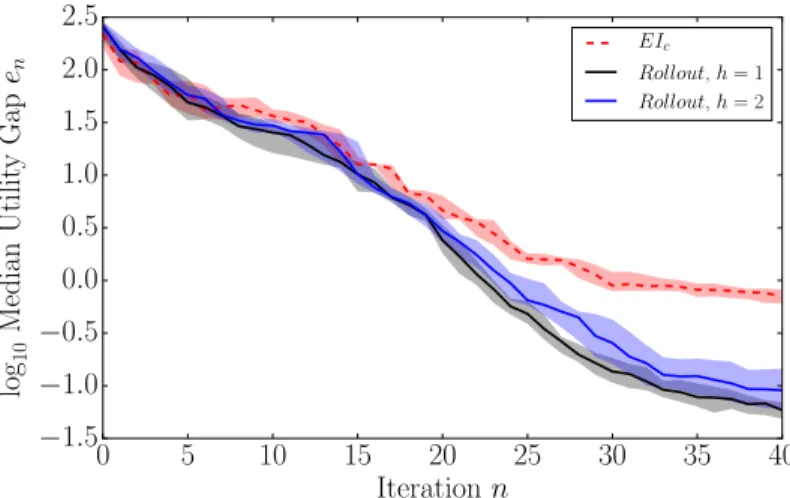
The optimization of the criterion is also a difficult problem because the EI criterion is known to be highly multi-modal and hard to optimize. Our proposal is to conduct

The AGILE 4.0 project is the AGILE (2015-2018) follow-up project that intended to develop the next generation of aircraft multidisciplinary design and optimization

The ability of the criterion to produce optimization strategies oriented by user preferences is demonstrated on a simple bi-objective test problem in the cases of a preference for

The extended domination rule makes it possible to derive a new expected improvement criterion to deal with constrained multi-objective optimization problems.. Section 2 introduces

First, the input point cloud is aligned with a local per-building coordinate system, and a large amount of plane hypothesis are detected from the point cloud using a random sam-