HAL Id: hal-01683103
https://hal.archives-ouvertes.fr/hal-01683103
Submitted on 12 Jan 2018
HAL is a multi-disciplinary open access
archive for the deposit and dissemination of
sci-entific research documents, whether they are
pub-lished or not. The documents may come from
teaching and research institutions in France or
abroad, or from public or private research centers.
L’archive ouverte pluridisciplinaire HAL, est
destinée au dépôt et à la diffusion de documents
scientifiques de niveau recherche, publiés ou non,
émanant des établissements d’enseignement et de
recherche français ou étrangers, des laboratoires
publics ou privés.
A physical-based constitutive model for surface integrity
prediction in machining of OFHC copper
Lamice Denguir, José Outeiro, Guillaume Fromentin, Vincent Vignal, Rémy
Besnard
To cite this version:
Lamice Denguir, José Outeiro, Guillaume Fromentin, Vincent Vignal, Rémy Besnard.
A
physical-based constitutive model for surface integrity prediction in machining of OFHC
cop-per.
Journal of Materials Processing Technology, Elsevier, 2017, 248 (octobre), pp.143-160.
Accepted Manuscript
Title: A physical-based constitutive model for surface integrity
prediction in machining of OFHC copper
Authors: L.A. Denguir, J.C. Outeiro, G. Fromentin, V. Vignal,
R. Besnard
PII:
S0924-0136(17)30174-7
DOI:
http://dx.doi.org/doi:10.1016/j.jmatprotec.2017.05.009
Reference:
PROTEC 15217
To appear in:
Journal of Materials Processing Technology
Received date:
13-4-2017
Accepted date:
11-5-2017
Please cite this article as: Denguir, L.A., Outeiro, J.C., Fromentin, G., Vignal, V.,
Besnard, R., A physical-based constitutive model for surface integrity prediction
in machining of OFHC copper.Journal of Materials Processing Technology
http://dx.doi.org/10.1016/j.jmatprotec.2017.05.009
This is a PDF file of an unedited manuscript that has been accepted for publication.
As a service to our customers we are providing this early version of the manuscript.
The manuscript will undergo copyediting, typesetting, and review of the resulting proof
before it is published in its final form. Please note that during the production process
errors may be discovered which could affect the content, and all legal disclaimers that
apply to the journal pertain.
Journal of Materials Processing Technology xxx (201x) x-x
A physical-based constitutive model for surface integrity prediction in machining of OFHC
copper
L.A. Denguir
a,b*, J.C. Outeiro
a, G. Fromentin
a, V. Vignal
b,d, R. Besnard
c,da LaBoMaP, Arts et Metiers, Campus of Cluny, Rue Porte de Paris, 71250 Cluny, France
b ICB, UMR 6303 CNRS - Université de Bourgogne Franche-Comté, BP 47870, 21078 Dijon, France c CEA, DAM, Valduc, 21120 Is-sur-Tille, France
d Laboratoire Interactions Matériau-Procédé-Environnement, LRC LIMPE n° DAM-VA-11-02, France
* Corresponding author: Lamice.DENGUIR@ensam.eu
A R T I C L E I N F O A B S T R A C T Keywords: Constitutive Model; OFHC Copper; Orthogonal Cutting; Modelling; Surface Integrity.
Due to the rising interest in predicting machined surface integrity and sustainability, various models for metal cutting simulation have been developed. However, their accuracy depends deeply on the physical description of the machining process. This study aims to develop an orthogonal cutting model for surface integrity prediction, which includes a physical-based constitutive model of Oxygen Free High Conductivity (OFHC) copper. This constitutive model incorporates the effects of the state of stress and microstructure on the work material behavior, as well as a dislocation density-based model for surface integrity prediction. The coefficients of the constitutive model were identified through a hybrid experimental/numerical approach, consisting in mechanical tests, numerical simulations and an optimization-based algorithm. The orthogonal cutting model was simulated by FEM, using ALE formulation, and was validated by comparing predicted and measured results, including residual stresses, dislocation density and grain size. The model is then used to analyze the influence of the cutting parameters and cutting geometry on surface integrity, and its results are compared to those obtained by the Johnson-Cook model.
1. Introduction
Predicting the machined surface integrity and durability is of prime interest while producing components destined to critical applications requiring high safety and endurance levels such as nuclear energy. Researchers have performed several and various models for metal cutting simulations. However, it is worth to notice that their accuracy to predict the machining performance (including surface integrity) is tightly related to the effectiveness of these models in representing the actual metal cutting process (Jawahir et al. 2011) (Outeiro et al. 2015a). In fact, such models are sensitive to several factors, including the description of the work material behavior during the cutting process, usually
represented through a constitutive (material) model. The classical thermo-viscoplastic Johnson and Cook (J-C) constitutive model (Johnson and Cook 1983) is often adopted in metal cutting simulations. Its simplicity in addition to the availability of its parameters for various metals
Contents lists available at ScienceDirect
Journal of Materials Processing Technology
justify its wide use. Nevertheless, several studies highlighted the limits of the J-C model, as it doesn’t consider the material microstructure effects on the work material mechanical behavior.
One of the first constitutive models to consider microstructure is the Zerilli and Armstrong (1987) model (Z-A), developed for bcc (Iron) and fcc (Copper) metals. Follansbee and Kocks (1988) proposed a physical based thermo-viscoplastic model, called mechanical threshold stress (MTS), which involves athermal stress and thermal stress basing on dislocation generation and dynamic recovery. Gourdin and Lassila (1991) improved the Follansbee and Kocks (1988) model by using the Hall-Petch law to estimate that athermal stress and they applied it for
simulating compression tests of Oxygen Free High Conductivity (OFHC) Copper. Later, Andrade et al. (1994) modified the J-C model by concatenating it to a function of the dynamic recrystallization as it alters the flow stress when the recrystallization threshold is overcome in
OFHC copper forming, but it supposes that recrystallization occurs anyway at half fusion temperature. However, the previously presented
models don’t establish the relationship between the thermo-mechanical loading, the grain size and the micro-hardness, as they are affected by the machining process. Estrin et al. (1998, 2008) developed a model able to predict microstructure evolution of OFHC copper while ECAP forming. This model links the flow stress to dislocation density, which is divided into dislocations inside the material cells and dislocations at cells walls. Their evolution rates are ruled by a set of differential equations including the grain size, strain rates and temperature. Ding et al. (2011) adapted this model to cutting operations modelling. They applied it to predict grain refinement and dislocation density of several materials using several severe plastic deformation processes including cutting (Ding and Shin 2011, 2012a, 2012b). It enabled them to evaluate the impact of different cutting conditions on the microstructure of the machined materials. Recently, Rotella and Umbrello (2014) proposed a constitutive model for numerical simulations of machining. This model was used to predict microstructural changes (grain size and micro-hardness) induced by cryogenic and dry cutting of Ti6Al4V alloy. When compared to the complex material plasticity model of Farrokh and Khan (2009) that inspired them, this model considers the effects of microstructure evolution (grain size) in flow stress with a single equation having much less coefficients to identify. However, as it is a phenomenological model whose coefficients were calibrated to fit turning operation results without performing material characterization tests, its applicability to other operations still need to be proven. Liu et al. (2014a)
proposed a called Unified Physical Model used in the numerical simulations of OFHC copper machining. It relates stresses including its both parts (athermal and thermal), dislocation densities, dynamic recrystallization and dynamic recovery besides the grain size evolution in a set of inter-related equations. Although this model is physical-based and shows good prediction results, its high number of parameters and its calibration complexity makes it intricate to put in practice. Bacca et al. (2015) proposed a new microstructure model estimating the grain size at severe plastic deformation and applied it to the FE simulation of machining aluminum alloy Al6061-T6, however, its limited to large plastic deformation of metals subject to negligible annealing effects. Atmani et al. (2016) proposed a multi-physics modelling of metal cutting. They described the flow stress of the work material by the MTS model. In order to predict the work material grain size evolution during machining, they used a mixture of the physical-based Dislocation Density model and the MTS model. Nevertheless, Bai and Wierzbicki (2008) demonstrated recently that the state of stress, represented by the stress triaxiality and the Lode angle (third deviatoric stress invariant)
parameters, has a non-negligible influence on the metal plasticity and fracture. They proposed a new asymmetric plasticity and fracture models (B-W) including corrections for hydrostatic pressure and the Lode parameter bringing an enhancement in the predicted results that reaches 20% for aluminum 2024-T351. They reported that it could be attributed to the effect of hydrostatic pressure on metal crystal dislocations and asymmetric fracture locus. Their models have been used in metal cutting simulations. Liu et al. (2014b) used them to simulate orthogonal
cutting of 2024-T3 aluminum alloy and found that the B-W fracture model with consideration of rate dependency, temperature effect and damage evolution gives the best prediction of chip removal behavior of ductile metals comparing to 4 other ductile fracture models. Although they presented results concerning to the workpiece temperature, von Mises and pressure stresses besides the generated surface roughness, no data have been shown concerning to the residual stresses or microstructure prediction. Buchkremer et al. (2016) made an extended Modified Bai-Wierzbicki material model (MBW) to simulate chip breakage while turning AISI 1045 with different cutting inserts and evaluate the influence of state of stress as well as damage on the strain hardening behavior. However, in their work, no surface integrity results have been reported concerning to the generated surface.
In the current work a physical-based constitutive model is proposed and applied to the orthogonal cutting simulation of OFHC copper. For accurate prediction of the surface integrity, this model considers the effects of strain, strain rate and temperature formulated by J-C, completed with the microstructure transformation and the state of stress effects, to capture the work material mechanical behavior in machining. The coefficients of the constitutive model are identified through a hybrid experimental/numerical approach, consisting in mechanical tests, numerical simulations and an optimization-based algorithm. Result of the numerical simulation of orthogonal cutting using this material constitutive model are presented and compared to the experimental results. The performed tests are then used to explain the effect of the variation of the uncut chip thickness and the tool rake angle on the surface integrity induced by the machining process. The results of the proposed model are compared to those obtained by the Johnson-Cook (1983) model for OFHC copper.
2. Physical-based constitutive model formulation
2.1. Plasticity model formulation
The proposed material constitutive model takes into consideration the most relevant phenomena influencing the material behavior. It was inspired from phenomenological models considering the strain hardening, the strain-rate, the temperature (Johnson and Cook 1985), the microstructural transformation (Andrade et al. 1994), and the state of stress effects (Bai and Wierzbicki 2008). The flow stress 𝜎̅ is expressed by the following equation (Eq. (1)).
(1)
In this expression, the terms related to the strain hardening effect, viscosity effect and thermal softening effect are similar to the J-C model (Johnson and Cook 1985), where A represents the yield stress, B and n the material strain hardening coefficients, ε the strain, C the viscosity coefficient, 𝜀̇ the strain rate, 𝜀0̇ the reference strain rate, T the temperature, Tm the material melting temperature, Troom the room temperature, and
m the thermal softening coefficient.
However, as far as the microstructural effect on flow stress is concerned, Andrade et al. (1994) proposed a function (H(T)) traducing the microstructural transformation effect on the flow stress. It depends only on recrystallization temperature supposed to be equal to (Tm/2) as an
activation threshold, and the ratio (𝐻̂) between the flow stress just before recrystallization (σdef) and just at recrystallization (σrec). In the model
temperature as three of them influence the microstructural transformation. Indeed, it is activated by the function u (Eq. (3)) only in case the strain exceeds the recrystallization strain threshold (εr), calculated using the equation proposed by Liu et al. (2015) for OFHC copper (Eq. (6)),
which is more accurate than using (Tm/2) as recrystallization threshold. Then, 𝐻̂ is completely substituted by the function 𝐻̂(𝜀, 𝜀̇) (Eq. (4))
where there is no need to define σdef and σrec.
(2)
(3)
(4) (5)
(6)
The coefficients hi (i=0..2) and ej (j=0..3) are material constants. Their values are determined by the identification process described in
§2.1.2. Concerning to the effect of the state of stress, only the stress triaxiality, η (the ratio between hydrostatic stress and von Mises equivalent stress) is considered. In fact, only the term (1-cη.(η-η0)) is taken from the B-W plasticity model (Bai and Wierzbicki 2008) where η designates
the stress triaxiality, η0 the reference triaxiality, and the triaxiality coefficient cη proper to the material. This term reflects the effect of hydrostatic pressure on the metal dislocations (Bai and Wierzbicki 2008).
2.1.1. Experimental setup for material characterization
The elasticity modulus (E) is determined using BING technique that is based on a vibratory method (da Silva et al. 2012). In fact, the beam remains on two elastic supports, then a mechanical choc is applied to the specimen extremity, making the beam vibrate. A microphone collects then acoustic data and transforms them into an electrical signal. Knowing the geometrical dimensions, the mass and the first vibration mode, by applying the beams theory, elasticity modulus is defined. This modulus is automatically calculated using the software SISTER®.
The yield stress is determined using a conventional tensile test respecting the ISO 3167 standard with a type A specimen. The used test machine is INSTRONTM 1185 model. The test velocity is 5 mm/min. Strain is measured by the incremental extensometer Zwick/RoellTM
Clip-On Inka.
Compression tests performed on the GleebleTM machine 3500 model are used to characterize the material’s stress-strain response at low and
intermediate strain rates (up to 100 s-1). The specimen is put between hot anvils fixed on the machine jaws. To enhance the conductivity and
reduce friction at the jaw/specimen interface, a graphite paper and a nickel paste are inserted in each interface. The GleebleTM machine is
equipped with a heating system to evaluate the influence of temperature on stress-strain. The used specimens are cylindrical with a diameter of 6 mm and a height of 9 mm. Thermocouples are welded to the specimens in order to control the tests temperatures. The varying parameters are the temperature (20°C, 200°C, 400°C and 600°C) and the strain-rate (0.1 s-1, 1 s-1 and 10 s-1). 12 tests are performed with one repetition for each
tested condition.
Split Hopkinson Pressure Bars tests (SHPB) (Hopkinson 1914) (Kolsky 1949) are used to characterize the material response at high strain-rates (up to 104 s-1) (Klepaczco et al. 1993). The setup, the detailed description of the test and its results exploitation method are reported by
u(
e
,T )
=
0
whene
<
e
r(
e
,T )
1
whene
³
e
r(
e
,T )
ì
í
ï
îï
ü
ý
ï
þï
Jaspers and Dautzenberg (2002). The geometry of the used specimens is the same as the one used for compression tests using the Gleeble machine. The tested strain-rates are 600 s-1, 700 s-1, 1600 s-1 and 2000 s-1. The tested temperatures are 200°, 400°, 500°C, 600°C and 650°C.
Quasi-static tensile tests at room temperature using flat grooved double notched specimens are performed on Zwick/RoellTM Z250 machine
to evaluate the material’s force-displacement response at different stress triaxiality conditions. In fact, for each specimen, stress triaxiality η can be estimated by Eq. (7), in function of the radius (R) and the thickness (t) illustrated in Fig. 1 (Bai and Wierzbicki 2008).
(7)
In this case, two specimens with different notches geometries are used: one with t = 3 mm and R = 3 mm, the other with t = 2 mm and R = 6 mm. Using Eq. (7), the first specimen geometry (t = 3 mm and R = 3 mm) corresponds to a stress triaxiality (η) of 0.84, while the second specimen geometry (t = 2 m and R = 6 mm) to 0.67.
2.1.2. Identification of the plasticity constitutive model’s coefficients
The proposed plasticity model coefficients (A, B, C, n, m, hi (i=0…2) and cη) are identified based on the procedure represented in Fig. 2, which consists into an identification of the initial values of the model coefficients using a direct method, followed by the application of an optimization-based indirect method to identify the final values of the coefficients. So, the direct method is used only to identify the initial values of the coefficient, which will be used in the optimization-based method to improve its convergence (Bariani et al. 2004).
The initial values of the model coefficients are identified as follows:
To identify the coefficients corresponding to the strain hardening effect, stress-strain data from both tensile and compression tests at room temperature (20°C) and quasi-static deformation conditions were used. The tensile test permitted to determine the yield stress, represented by the coefficient A. The stress-strain data obtained from the compression tests using the Gleeble machine at a reference strain rate 𝜀̇0 equal to 0.1 s -1, permitted to determine the coefficients B and n. To identify the coefficient C, corresponding to the strain-rate effect, both stress-strain data
from compression tests using Gleeble machine and SHPB apparatus at room temperature and different strain-rates were used. The several temperatures values aim to identify the thermal softening coefficient m, as well as those parameters related to the dynamic recrystallization, hi (i
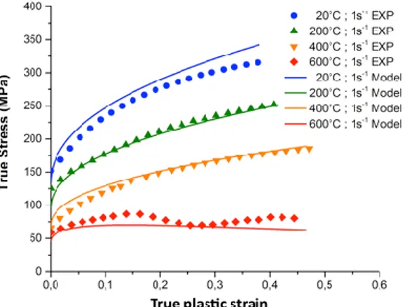
= 0…2). To find the values of hi coefficients, stress-strain data obtained at a testing temperature around 600°C is used due to the favorable
temperature conditions for dynamic recrystallization (temperature superior than recrystallization threshold temperature). Experimental results at 600°C in Fig. 3 show that dynamic recrystallization may exists for that temperature, since a decrease in the stress is observed when the strain increases (Andrade et al. 1994).
After identifying the initial values of the strain hardening, strain-rate, thermal softening and recrystallization coefficients, the above-mentioned optimization-based method is used to identify the final values. This optimization-based method consists into simulating the compression test and modifying the constitutive model coefficients iteratively using a Genetic Algorithm (GA), In order to minimize the difference between the predicted and measured force-displacement curves. So, numerical simulations of compression test are performed on ABAQUS, using a developed Fortran subroutine VUMAT for calculating the flow stress data given by Eq. (1), without the state of stress effect. The model coefficients (A, B, C, n, m and hi) to be identified are inserted in the ABAQUS input file as parameters, which are modified by GA,
implemented in the LS-OPT optimization software. The initial values used in this optimization-based method are those identified with the experimental data using least squares fitting method. Optimization software launches automatically ABAQUS simulation, collects the simulated forces-displacement curve, and compares it with the experimental one. In function of the deviation between the obtained simulated and
experimental curves, the optimization software seeks the optimal values of the constitutive model coefficients, in order to minimize this deviation. The values of the model coefficients are considered as satisfying when this deviation is less than 10%.
The same procedure is used to identify the state of stress coefficient (cη). So, the initial value of cη is identified using the direct method,
followed by the application of the optimization-based indirect method to identify the final value of this coefficient. Firstly, the reference stress triaxiality η0 corresponding to that one on compression of cylindrical specimen is used (-0.33 according to Bai and Wierzbicki (2008)). Then,
the coefficient cη is identified basing on the previous procedure, using the curves issued from tensile tests performed on double notched flat specimen. Both specimen’s geometries are used in the identification of cη, and the final value of this coefficient is obtained when the difference between the predicted and measured force-displacement curves is less than 10%.
All the identified coefficients are gathered in Table 1(except the coefficients ei that are taken from the literature Liu et al. (2015)).
2.2. Damage model formulation
Damage and fracture of a ductile material are explained by the formation of microscopic voids inside the material followed by their growth and their coalescences under a triaxiality state of stress. Their growth initiates micro-cracks in a progressive way leading to fracture (Rice and Tracey 1969). Fig. 4 demonstrates a hypothetic stress–strain curve shown by the dashed line where no damage occurs. In the same figure, the real curve corresponds to a conventional (real) uniaxial stress test, and is shown by the solid line. The elastic–plastic undamaged path (abc) is followed by the separation of the experimental yield stress from the virtual undamaged yield stress at point ‘c’. In fact, hypothetic damage initiation site where the material hardening modulus becomes progressively sensitive to the amount of damage leading to the declination of the material loading capacity occurs in point ‘c’. It also marks the start of elasticity modulus degradation. Due to the increased damage, the material reaches its ultimate stress capacity at point ‘d’ where the hardening modulus becomes zero. Point ‘e’ denotes the observed fracture initiation site and finally point ‘f’ indicates the failure.
To detect strain at damage initiation, εf, the J-C damage model (Johnson and Cook 1985) is used, which depends on stress triaxiality
(MacClintock 1968), strain-rate and temperature, given by Eq. (8):
(8)
where Di (i = 1…5) are the coefficients identified basing on fracture tests, η is the stress triaxiality, 𝜀̇𝑝 is the plastic strain rate, 𝜀̇0 is the reference
strain-rate, T is the temperature, T0 is the room temperature and Tm is the melting temperature. The material is assumed to start the strain
softening and degradation when the damage indicator ω reaches 1. This parameter is defined by the following cumulative law (Eq. (9)):
where Δεp is the increment of the equivalent plastic strain while a charge increment j at the integration point i. Then, the material strength
degradation behavior beyond damage initiation is controlled by the parameter D. It is used to describe the material flow past damage initiation by the following relationship (Eq. (10)):
(10) where 𝜎̅ℎis the hypothetic undamaged stress estimated by Eq. (1).
As far as damage evolution is concerned, Hillerborg et al. (1976) fracture energy (Gf) is adopted in the calculus of the damage parameter D
as following in Eq. (11):
(11)
with L the characteristic length of the square root of the finite element area, 𝜀̅p the plastic strain, 𝜀̅pB plastic strain at damage initiation, 𝑢̅p the
plastic displacement and 𝜎̅ the equivalent von Mises stress. The characteristic length is depending on the size of the considered mesh element. Therefore, the user should carefully manipulate the elements size and perform the necessary mesh refinement to minimize the error induced by such approximation.
The model formulation grants that energy dissipation is equal to Gf while damage evolution. For plan strain, Gf can be obtained by the
following equation (Eq. (12)):
(12)
with Kc the tenacity, υ the Poisson coefficient and E the elasticity modulus.
The damage coefficients (D1 to D5) values used in the numerical simulation are identified by Johnson-Cook (1985) and
Hohenwarter-Pippan (2015) for the OFHC copper, and shown in Table 2. The Young’s modulus was identified experimentally using the Bing test, as described previously.
2.3. Microstructure prediction model formulation
The microstructure parameters are predicted using the dislocation density based model proposed by Estrin et al. (1998). It aims to calculate the total dislocation density ρtot evolution and grain size, d. It makes a distinction between the two kinds of dislocations: those in the cells walls,
ρw, and those in the cells interiors, ρc. Knowing the volume fraction of dislocation cells walls (f) defined by Eq. (13), the total dislocation density
can be calculated using Eq. (14).
(13)
(14)
where f∞ is the saturation value of f, f0 is the initial value, and 𝛾̅𝑟 is the reference resolved shear strain γr. The resolved shear strain (γr) can be
calculated knowing the resolved shear strain-rate (𝛾̇𝑟), using the following equation:
where 𝜀̇ is the strain-rate, Mt is the Taylor factor (Ding and Shin 2012b). Volume dislocation densities in the cells (ρc) and in the walls (ρw) are
governed by two differential equations based on the reactions that are susceptible to occur due to dislocation nucleation, annihilation and interaction between dislocations. Dislocations density evolution are given by the following equations:
(16)
(17)
where the first terms on the right side correspond to the generation of dislocations due to the activation of Frank–Read sources. The second terms denote the transfer of cell interior dislocations to cell walls where they are woven in. The last terms in each of the evolution equations represent the annihilation of dislocations leading to dynamic recovery in the course of straining. α*, β* and ko are dislocation evolution rate
control parameters for the material, n is a temperature sensitivity parameter, f is the volume fraction of the dislocation cell wall calculated by Eq. (13), b is the magnitude of the Burgers vector of the material, d is the dislocation cell size and 𝛾̇̅𝑟 is the reference resolved shear strain-rate. It is
assumed that the resolved shear strain-rate (𝛾̇𝑟) across the cell walls and cell interiors are equal, which satisfies the strain compatibility along the
interface between interiors and boundaries.
In order to calculate the grain refinement induced by machining, the average grain size (dgrain) is assumed to be inverse proportional to the
square root of the total dislocation density (Ding and Shin 2011), as shows Eq. (18).
(18)
Knowing the bulk material initial grain size determined by the optical microscopy, the initial dislocations density determined by X-ray diffraction and applying the method proposed by Ding and Shin (2012b), the values of K, f0, f∞, ρc0, ρw0, 𝛾̅𝑟
and
𝛾̇̅
𝑟are calculated. The variable values are listed in Table 3, where the values of the α*, β* and b are taken from literature (Ding and Shin 2012b).3. Orthogonal cutting model and tests
The proposed physical-based constitutive model was implemented on an orthogonal cutting model, to evaluate its effectiveness to predict the surface integrity induced by machining OFHC copper. The following sections describe this orthogonal cutting model and the corresponding machining tests used to validate it.
3.1. Orthogonal cutting model
A 2D orthogonal cutting model of OFHC copper was developed and simulated using the Finite Element Method (FEM) and the Arbitrary Lagrangian–Eulerian (ALE) formulation. A coupled temperature displacement analysis was performed using ABAQUS/Explicit FEA software.
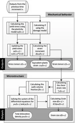
To model mechanical behavior and microstructure evolution of OFHC copper, a user subroutine VUMAT was developed integrating the physical-based constitutive model described in §2. The structure of this subroutine is shown in Fig. 5.
As far as the tool is concerned, it was modelled as elastic and its thermal and elastic properties were taken from literature (Mabrouki et al. 2008) and listed in Table 4.
The varying cutting parameters are the uncut chip thickness, h (0.05 mm and 0.2 mm), and the tool rake angle rake, γ (20° and 30°). The fixed cutting parameters are the cutting speed Vc (90 m/min) and the cutting-edge radius rn (10 µm).
During cutting simulations, with the use of adaptive meshing related to the ALE formulation, no chip separation criterion was used. However, the utility of the use of a damage law in this simulation consisted in correcting and limiting the flow stress in order to model the real behavior of the machined material.
The workpiece was meshed with quadrilateral continuum elements CPE4RT, while the tool was meshed with three nodes elements CPE3T. The total number of elements depended of the tool and workpiece geometry (between 10 000 and 14 000 elements). The regions needing mesh refinement (first and second deformation zones, and machined surface layer) contain the smallest elements size of 2 µm. The refinement was utilizing a bias of 10 along a depth of 200 µm beneath the machined surface.
Fig. 6 illustrates the used boundary conditions. Cutting speed was applied to the left side of the workpiece and the tool was considered as fixed. The workpiece green lines represent Lagrangian sliding surfaces, while the red lines represent Eulerian surfaces. An initial temperature of 20°C was imposed to both the tool and the workpiece.
Concerning to the tool-chip and the tool-workpiece contacts, they were modelled using the Zorev’s model (Zorev 1966). The value of the friction coefficient between the OFHC copper and the uncoated tungsten carbide (material of the cutting tool) was determined using special tribological tests to reproduce identical contact conditions as those found in machining, as described by Rech et al. (2013). These tests enabled the determination of the apparent friction coefficient (μapp), which includes both contributions of interfacial (local) adhesive phenomena (μadh)
and macroscopic plastic deformation (μplast). For cutting simulation, μadh was used; for the range of sliding velocities and contact pressures
applied in the machining tests, this coefficient can be represented as a function of the sliding velocity (vs), given by Eq. (19) (Denguir et al.
2016):
(19)
where the coefficients ci (i = 1..4) are equal to 0.787, 0.185, 0.764 and 0.362, respectively. It is worth to notice that the proposed equation
follows the general trend of the friction coefficient with respect to the sliding velocity found by Zorev (1966). Concerning the limit shear stress (τlimit), it is equal to the yield shear stress (τy = σy/√3) and was calculated based on the estimated yield stress (σy) of the deformed superficial
layers of the chip and the machined surface. This yield stress is calculated by the used subroutine.
To model the air cooling generated by the vortex system, the free surfaces were immerged in a temperature of -5°C (268°K), and a convection coefficient of 81 W/(m2 K) was imposed at air/workpiece interfaces, as shown in Fig. 6. These values were estimated basing on experimental
measurements and heat transfer calculations. Based on temperature measurements using a thermocouple, the workpiece surface temperature was -5°C (268°K). To estimate the heat convection coefficient, hf, the following equation proposed by Astakhov (2006) was used:
where be is the equivalent length (in m), g is the gravity (in m2/s), and the other parameters are properties of the cooling fluid: vf the fluid
velocity (in m/s), kf thermal conductivity (in W/mK), γf density (in kg/m3), υf dynamic viscosity (in Pa.s) and cp the specific heat (in J/kgK).
Remaining on Eq. (19).
To calculate residual stresses, the workpiece had to be mechanically unloaded (Vc = 0 m/min), and its temperature had to reach the ambient
temperature. To reach stresses equilibrium in the shortest time, implicit formulation was used. So, the workpiece was transferred to ABAQUSTM/Standard, including the field variables and the mechanical behavior of the material. Boundary conditions were the ambient
temperature, zero displacement at the boundaries of the workpiece and a free surface at the machined surface. However, to model the workpiece material behavior, an equivalent UMAT subroutine was created.
3.2. Orthogonal cutting tests and analysis
To validate the numerical simulations, orthogonal cutting tests in planing configuration were performed on flat specimens (40x15x4 mm) of
OFHC copper (annealed at 450°C or 2 hours, with an average grain size of 55 μm), using a DMG DMC85V milling machine.
Uncoated cemented tungsten carbide cutting tools with two different geometries were used. Both tool geometries were characterized by an edge radius (rn) of 10±2 μm, a flank angle (α) of 10°, but different rake angle values (γ), one with of 20° and the another with 30°. Two uncut
chip thickness (h) values of 0.05 and 0.2 mm were used. The cutting speed (vc) and the width of cut (W) was kept constant and equal to 90
m/min and 4 mm, respectively. Low temperature pressurized air (-5±2°C; 6 bar) cooling generated by a vortex system was applied to minimize the adhesion phenomenon between the tool and the work material.
The orthogonal cutting tests permitted to generate the following data for machining model validation: i) Chip Compression Ratio (CCR); ii) residual stresses; iii) dislocation density; and iv) grain-size.
Chip compression ratio (CCR) is a quantitative measurement of the total plastic deformation reached in the cutting (Astakhov and Shvets 2004). Due to the irregular chip thickness obtained while the orthogonal cutting tests, the CCR was calculated based on the ratio between the chip cross-section and the uncut chip cross-section. A Matlab® script was developed in order to find the real area of the polished chip cross
section basing on its numerical image taken by the high digital resolution image microscope Keyence VHXTM.
Residual stresses were determined using PROTOTM IXRD diffractometer, based on the X-ray diffraction technique and applying the sin2ψ
method. According to this method, the residual stresses were calculated from strain distribution εφψ{hkl} derived from the measured inter
reticular plane spacing and knowing the elastic radio crystallographic constants, S1{hkl} and ½S2{hkl}, which are equal to -3.13×10⁻⁶ MPa-1 and
11.79×10⁻⁶ MPa for OFHC copper, respectively. An X-ray Mn-Kα radiation (18 kV at 4 mA) was used to determine the elastic strains in the
(311) planes (149.09° Bragg angle). Residual stresses were determined in the machined surface and subsurface, in the cutting direction and parallel to the cutting edge. To determine the in-depth residual stress profiles, successive layers of material were removed by electro-polishing, to avoid the reintroduction of residual stress. Further corrections to the residual stress data were made due to the volume of material removed (Moore and Evans 1958).
To evaluate the dislocation density, a measurement of the Bragg peak broadening of the dislocation/defect density in the diffracting domain by X-ray diffraction was performed. In fact, for a simple Gaussian distribution, the full width at half maximum (FWHM) may be related to the dislocation density (ρ) when the model of Williamson and Smallmann (1956) is used. This model considers the FWHM as in Eq. (22):
(22)
with <ε2>1/2 the distortion in a given direction induced by the defaults around the coherent domains and θ the Bragg angle. The dislocation
density (ρ) is then given by Eq. (23):
(23)
with c a parameter of dislocations distribution equal to 12 for face-centered cubic crystalline structure of the copper, D the size of the perfect crystalline domain in a crystallographic direction, b the Burger’s vector (equal to 2.57×10⁻¹⁰ m for copper), and L to designate the total length of
the column on which internal inelastic distortions are averaged. To find the parameter D, the method developed by Delhez et al. (1982) was used.
The grain size measurements were performed using the optical microscope OLYMPUSTM BX51M. In order to evaluate the evolution of the
grain size in function of the depth beneath machined surface, the following procedure was adopted. First, the machined surface was polished and etched by the electro-polishing machine StruersTM LectroPol-5 using the electrolyte StruersTM D2 (phosphoric acid), suitable for copper and
copper alloys. Second, the thickness of the removed layer was measured using a comparator with a mechanical probe with a resolution of 1 µm. Third, the surface was observed by an optical microscope equipped with a polarizing filter. Finally, the image issued from optical microscopy was numerically treated to identify grains walls and calculate the area of each grain. A statistical treatment gives the average grain area and the equivalent grain size corresponding the length of the edge of a square having the same area as the average grain area. This definition of the grain size is used in all the results.
4. Comparison between predicted and measured results
4.1. Chip Compression Ratio
Fig. 7 shows both the measured and predicted CCR for three cutting conditions corresponding to two rake angles and two uncut chip thickness values. For the same cutting conditions, the predicted CCR is almost similar to the measured one, except the slight difference seen in the CCR when the uncut chip thickness h is equal to 0.05 mm (20% overestimated).
However, in order to fully validate the orthogonal cutting model, a comparison between predicted and measured machined surface integrity features (residual stresses, dislocation density and grain size) is required.
4.2. Residual stresses
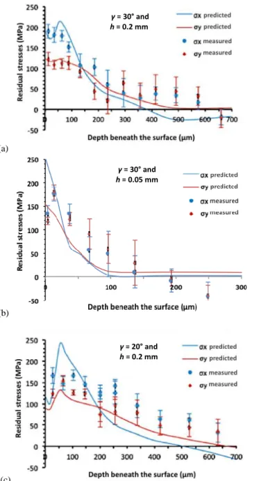
To validate the predicted residual stresses, three experimental in-depth residual stresses profiles, corresponding to three different cutting conditions, are used. Measured and predicted in-depth residual stress profiles are shown in Fig. 8(a), (b) and (c) in both cutting (σx) and
transversal (σy) directions. These figures show that, in general, the residual stresses are tensile at surface, increasing with the depth beneath
surface, reaching a maximum around 20-50 𝜇m. Then, they decrease as the depth beneath surface increase, reaching the residual stress state in the work material before machining (around zero). These figures also show that the orthogonal cutting model is reasonable capturing the shape
of the in-depth residual stresses distribution. An exception is observed for h equal to 0.05 mm, where the model shows problems in capturing the shape of the measured in-depth residual stress profile near the machined surface.
The observed differences between predicted and measured residual stresses can be justified as follows:
Difficulties in X-ray diffraction measurements for depths below surface greater than 200 µm, due to the high grains size of the base material (55 𝜇m).
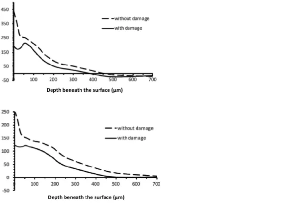
Since the damage model coefficients were taken from literature, they may not be accurately representing the behaviour of the work material used in the experimental tests. This will mainly affect the residual stress predictions near surface, and slightly at the subsurface. In fact, as shown in Fig. 9(a) and (b), damage effects significantly improve the predicted residual stress near the machined surface.
It seems that the uncut chip thickness strongly affects the residual stresses when it increases from 0.05 mm (Fig. 8b) to 0.2 mm (Fig. 8a). However, when the tool rake angle increases from 20° (Fig. 8c) to 30° (Fig. 8a), the residual stress slightly increases at the surface and decrease at the subsurface.
In order to explain the influence of both uncut chip thickness and tool rake angle on the residual stresses distributions, the thermal and mechanical actions of the cutting tool over the workpiece are investigated. In particular, the temperature and stress triaxiality distributions in chip formation and surface generation are evaluated in function of the uncut chip thickness and tool rake angle. These distributions are obtained from the numerical simulations.
As far as the temperature distribution is concerned, Fig. 10 shows that, for an uncut chip thickness of 0.05 mm. The maximal temperature at the machined surface (in contact with the tool clearance) is low, of 87°C (360°K). When the uncut chip thickness increases to 0.2 mm keeping the same rake angle of 30°, the temperature increases up to 107°C (380°K) (Fig. 10(a) and (b)). The same is seen when the rake angle decreases from 30° to 20°, keeping the same uncut chip thickness of 0.2 mm, the surface temperature slightly increases from 107°C (380°K) to 117°C (390°K) (Fig. 10(b) and (c)). In fact, between both temperatures, flow stress drops by only 1.7%.
As the machined surface temperature varies so little with the tested cutting condition, residual stresses seem to be essentially generated by the mechanical loading induced by the cutting tool on the work material.
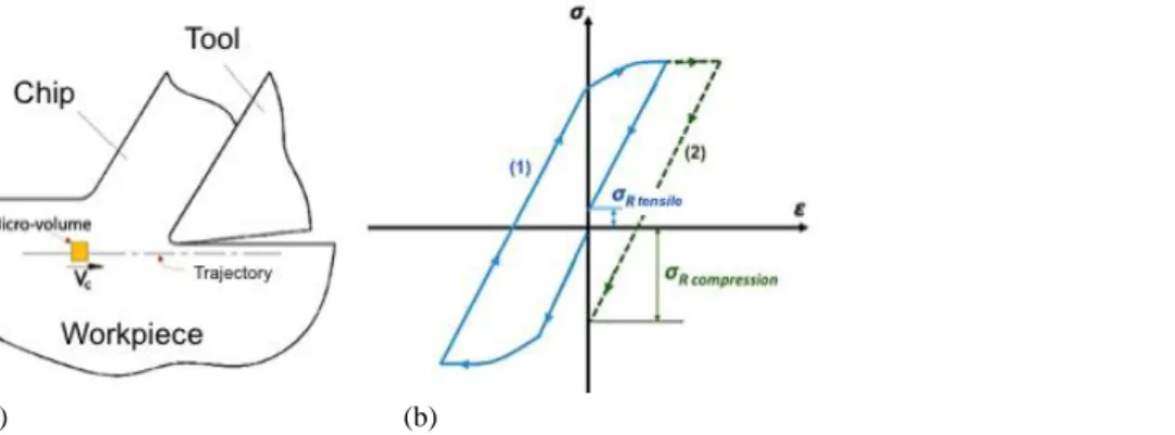
In order to understand the mechanism of residual stresses generated by the cutting process, the approach proposed initially by Liu and Barash (1976) and later by Matsumoto (1999) is adopted. According to Liu and Barash (1976), a simple method to describe the hardening process induced by machining consists in using stress-strain response obtained by a standard uniaxial tensile test. So, residual stresses in the machined surface and subsurface are the consequence of a compressive load followed by a tensile load at which a micro-volume of the work material animated by the cutting speed Vc is submitted, when it follows the trajectory represented in Fig. 11a. Fig. 11b shows schematically the level
reached by the residual stresses after a cycle of loading. Depending on the predominant loading type, the residual stress can be tensile or compressive. This representation (Fig. 11a) supposes that, after stress unloading, the elongation is equal to zero, so the length of the material element has always to remain unchanged before and after cutting (Liu and Barash 1976).
Considering that metal cutting is as forming process, which external energy applied to the cutting system causes the physical separation of the layer being removed (in the form of chips) from the rest of the workpiece. The process of physical separation of a solid body into two or more
parts is known as fracture, thus metal cutting must be treated as a deformation process until the fracture (Astakhov and Shvets 2004). Therefore, the fracture strain is an important mechanical property in metal cutting, which depends on the stress triaxiality in the chip formation zone. It can be suggested that fracture strain will influence the surface integrity, including residual stresses. In fact, the stresses triaxiality influence the fracture strain (see Fig. 12a) and consequently the residual stresses (see Fig. 12b).
According to the proposed model shown in Fig. 12a, a decrease in stresses triaxiality η implies an increase in the equivalent fracture strain εf,
consequently the residual stress σR comes up in the tensile direction. If it is a tensile residual stress, it just becomes higher, as shown in the
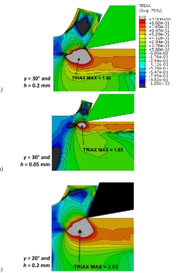
example presented in Fig. 12b. In fact, simulations show an increase in stresses triaxiality when the uncut chip thickness h increases from 0.05 mm to 0.2 mm and/or the rake angle γ decreases from 30° to 20° (Fig. 13), which lowers the work material fracture strain, thus reducing the residual stresses at the machined surface.
However, when it comes to the subsurface where εf is not reached, the work material is essentially submitted to hardening when the elastic
stress is overcome. That hardening depends on the applied mechanical loading. Since that loading is lower when h = 0.05 mm than when h = 0.2 mm, the residual stresses will be also lower for smaller uncut chip thickness. Nevertheless, for the same uncut chip thickness, the highest loading corresponds to the lowest rake angle (γ = 20°), which induces the highest residual stress at the subsurface.
4.3. Dislocation density and grain size
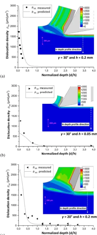
Using the analysis of the full width at half maximum of X-ray diffraction peaks, an experimental evaluation of dislocation densities is performed. Then, simulation results are compared to the experimental ones (Fig. 14a, b and c).
The presented results are given using the normalized depth, which is the ratio between the depth beneath the surface d and the uncut chip thickness h. Although simulations overestimate dislocation density values at the machined surface for the cases when h = 0.2 mm and
underestimate it when h = 0.05 mm, the general trends in function of the cutting conditions are in good agreement with the experimental results: the lowest dislocation densities beneath the surface are obtained for h = 0.05 mm and γ = 30°, the highest at surface for h = 0.2 mm, and the affected layer (where dislocation density is higher than that of the bulk material) is thicker for h = 0.2 mm and γ = 20°.
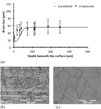
To compare the average grain size (dgrain), the experimental method described previously in paragraph §3.2 is adopted. It is reminded that a
grain size dgrain corresponds to the length of the edge of a square whose area is equivalent to the area of the considered grain (Toth et al. 2002).
Fig. 15 and Fig. 16 represent measured and predicted results for the cutting conditions shown in these figures. The shape of the in-depth distribution of the predicted grain-size is identical to the measured one. Concerning to the values, it is worth to notice that, experimentally, there is a high dispersion of the grain size (see Fig. 15b and c, then Fig. 16b and c).
As the process of microstructure evolution occurs under thermal and mechanical loadings, the differences seen in the machined surface and subsurface microstructures under the different tested cutting conditions can be considered as a result of the severe plastic deformation induced during the cutting process. In fact, as reported by Atmani et al. (2016), under the strain increase during cutting, the initial microstructure of an annealed metal upon machining with homogeneous distribution of dislocations in the grain evolves into elongated dislocations cell structures and generates new randomly distributed dislocations. Then, a development of dense and elongated sub-grains besides the formation of new grains occur.
As the plastic deformation is more severe at the machined surface for the cutting condition corresponding to γ = 20° and h = 0.2 mm comparing to the other tested ones, it is then normal that the resulting dislocations densities are the highest and the grain size recorded is the lowest comparing to the both other machined surfaces. Nevertheless, as the layer beneath the surface affected by the plastic deformation is deeper when γ = 20° and h = 0.2 mm (Outeiro et al. 2015b), consequently it is predictable to have a thicker layer where dislocations density is high comparing to the two other cases.
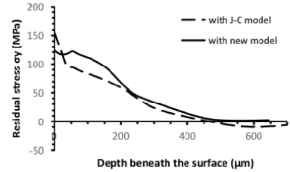
5. Comparison with the J-C model
The simulated results obtained by the physical-based constitutive model are here compared to those obtained by the Johnson-Cook model, which is widely used in machining simulations. Concerning to the residual stresses σx (Fig. 17a) and σy (Fig. 17b), the simulated results show
that the J-C model overestimates the residual stresses at the surface (up to 25% in the cutting direction) but at the subsurface, it provides lower estimated values, which proves that the newly proposed model gives better predictions.
Although there are small differences between orthogonal cutting simulations results, the extent of including the recrystallization effect in the material constitutive model can't be highlighted, unlike the case of hot material forming processes. In fact, the occurrence of the dynamic recrystallization process at the machined surface is not granted due to the low temperature of the material during cutting (Fig. 10). Indeed, while comparing compression tests simulations using both models (Fig. 18), it is worth noticed that the gap between the J-C and the proposed model results becomes larger when the test temperatures are higher. Especially when the recrystallization threshold is overcome, the J-C model can't be used (overestimation up to 100%) while the proposed model is still accurate (Fig. 3 and Fig. 18)
6. Conclusions and outlook
In the presented study, a physical-based constitutive model of OFHC copper is developed, which includes the plasticity, damage and microstructural behaviors. It includes the “classical” strain-rate and temperature effects, as well as the microstructural and the state of stress effects, in order to improve the surface integrity prediction induced by machining. A hybrid experimental/numerical approach consisting in mechanical tests, numerical simulations and an optimization-based algorithm has allowed to identify the proposed plasticity model coefficients. This constitutive model is integrated in an orthogonal cutting model and applied to predict the CCR and the surface integrity parameters, namely: residual stress, dislocation density and grain size. The comparison between predicted and measured results have shown that the proposed constitutive model gives better predictions when compared to the classical Johnson-Cook one.
A new model for residual stress formation in metal cutting is proposed based on the Liu and Barash model and considering the strain at fracture depending on the stress triaxiality. This model shows that residual stresses increase as stress triaxiality decreases, which occurs when h decreases and γ increases. However, at the subsurface where fracture is not occurring, the residual stress increases with the mechanical loading, which occurs when h increases and γ decreases. Concerning to dislocations densities and grains size in the machined samples, it has been found that grains are finer and dislocations are denser at the machined surface and for higher h.
As an outlook, the proposed constitutive model will be improved by conducting fracture tests under different strain-rates and stress triaxiality, in order to identify the coefficients of the J-C damage model, for the specific OFHC copper used in this study.
Acknowledgments
The authors would thank CEA Valduc for the financial and technical support. They also acknowledge Prof. A. C. Batista from the University of Coimbra, for the X-ray diffraction analysis.
References
Andrade, U. et al., 1994. Dynamic recrystallization in high-strain, high-strain-rate plastic deformation of copper. Acta Metallurgica Et Materialia, 42/9:3183– 3195.
Astakhov, V.P., 2006. Tribology of metal cutting B. J. Briscoe, ed., Elsevier.
Astakhov V. & Shvets S., 2004, The assessment of plastic deformation in metal cutting, J. of Materials Processing Technology, 146/2:193-202.
Atmani, Z. et al., 2016. Combined microstructure-based flow stress and grain size evolution models for multi-physics modelling of metal machining. Int. J. of Mechanical Science, 118:77-90.
Bacca M, et al., 2015, Continuous dynamic recrystallization during severe plastic deformation. Mechanics of Materials, 90:148–156.
Bai, Y. & Wierzbicki, T., 2008. A new model of metal plasticity and fracture with pressure and Lode dependence. Int. J. of Plasticity, 24/6:1071–1096. Bariani P.F. et al., 2004, Testing and Modelling of Material Response to Deformation in Bulk Metal Forming, CIRP Annals – Manufacturing Technology,
53/2:573–595.
Buchkremer S., Klocke F. & Veselovac D., 2016, 3D FEM simulation of chip breakage in metal cutting, Int. J. of Adv. Manufacturing Technology, 82:645-661. da Silva Leite E.R. et al. 2012, Estimation of the dynamic elastic properties of wood from Copaifera langsdorffii Desf using resonance analysis, CERNE,
18 :1 Lavras Jan./Mar. 2012.
Delhez, R., de Keijser, T.H. & Mittemeijer, E.J., 1982. Determination of crystallite size and lattice distortions through X-ray diffraction line profile analysis. Fresenius Z. Analytische Chemie, 312/1:1–16.
Denguir, L.A. et al., 2016. Orthogonal Cutting Simulation of OFHC Copper Using a New Constitutive Model Considering the State of Stress and the Microstructure Effects. Procedia CIRP, 46:238–241.
Ding H, Shen N. & Shin YC., 2011, Modeling of grain refinement in aluminum and copper subjected to cutting. Computational Materials Science, 50:3016–3025. Ding H. & Shin YC., 2011, Dislocation density-based grain refinement modeling of orthogonal cutting of commercially pure titanium. In: Proceedings of the
ASME International Manufacturing Science and Engineering Conference. Corvallis, Oregon, USA:MSEC2011-50220.
Ding H. & Shin YC., 2012a, Dislocation density-based modeling of subsurface grain refinement with laser-induced shock compression. Computational Materials Science, 53:79–88.
Ding H. & Shin YC., 2012b, A metallo-thermomechanically coupled analysis of orthogonal cutting of AISI 1045 steel. J. of Manufacturing Science and Engineering 134/051014.
Estrin Y. et al. 1998, A dislocation-based model for all hardening stages in larges strain deformation. Acta Materialia, 46/15:5509–5522. Estrin Y. et al., 2008, Strain gradient plasticity modelling of high-pressure torsion. J. of Mechanics and Physics of Solids, 56/4:1186–1202.
Farrokh, B. & Khan, A.S. 2009. Grain size, strain rate, and temperature dependence of flow stress in ultra-fine grained and nanocrystalline Cu and Al: Synthesis, experiment, and constitutive modeling, Int. J. of Plasticity 25, pp.715-732.
Follansbee PS & Kocks UF., 1988, A constitutive description of the deformation of copper based on the use of the mechanical threshold as an internal state variable. Acta Metallurgica, 36:81–93.
Gourdin WH & Lassila DH., 1991, Flow stress of OFE copper at strain rates from 10-3 to 104 s-1: grain-size effects and comparison to the mechanical threshold
stress model. Acta Metallurgica Et Materialia, 39/10:2337–2348.
Hillerborg, A., Modéer, M. & Petersson, P.-E., 1976. Analysis of crack formation and crack growth in concrete by means of fracture mechanics and finite elements. Cement and Concrete Research, 6/6:773–781.
Hohenwarter, A. & Pippan, R., 2015. Fracture and fracture toughness of nanopolycrystalline metals produced by severe plastic deformation Subject Areas: Phil. Trans. of the Royal Society A: Mathematical, Physical and Engineering Sciences, 373/2038: Article number 20140366.
Hopkinson B., 1914, A Method of Measuring the Pressure Produced in the Detonation of High Explosives or by the Impact of Bullets, Philosophical Transactions of the Royal Society (London) A, 213:437-456.
Jaspers, S.P.F.C. & Dautzenberg, J.H., 2002. Material behaviour in conditions similar to metal cutting: Flow stress in the primary shear zone. J. of Materials Processing Technology, 122/2–3:322–330.
Jawahir, I. S. et al., 2011, Surface integrity in material removal processes: Recent advances, CIRP Annals, 60/2:603–626.
Johnson GR & Cook WH, 1983, A constitutive model and data for metals subjected to large strains, high strain rates, and high temperatures. In: Proceedings of the 7th International Symposium on Ballistics. Hague, The Netherlands:541–547.
Johnson, G.R. & Cook, W.A, 1985. Fracture characteristic of three metals subjected to various strains, strain rates, temperatures and pressures. Engineering Fracture Mechanics, 21/1:31–48.
Klepaczko, J.R., Sasaki, T. & Kurokawa, T., 1993. On rate sensitivity of polycrystalline aluminum at high strain rates. Trans. of the Japan Society for Aeronautical and Space Sciences, 36:170–187.
Kolsky, H., 1949, An Investigation of the Mechanical Properties of Materials at Very High Rates of Loading, Proc. Phys. Soc., London, B62:676.
Liu, C.R. & Barash, M.M., 1976. The Mechanical State of the Sublayer of a Surface Generated by Chip-Removal Process—Part 1: Cutting with a Sharp Tool. J. of Engineering for Industry, 98/4:1192.
Liu R. et al., 2014a, The prediction of machined surface hardness using a new physics-based material model. Procedia CIRP, 13:249–56.
Liu J., Bai Y. & Xu C., 2014b, Evaluation of ductile fracture models in finite element simulations of metal cutting processes, J. of Manufacturing Science and Engineering, 136/011010:1-14.
Liu, R. et al., 2015. A unified material model including dislocation drag and its application to simulation of orthogonal cutting of OFHC Copper. J. of Materials Processing Technology, 216:328–338
Matsumoto, Y., Hashimoto, F. & Lahoti, G., 1999. Surface Integrity Generated by Precision Hard Turning. CIRP Annals - Manufacturing Technology, 48/1:.59– 62.
Mabrouki, T. et al., 2008. Numerical and experimental study of dry cutting for an aeronautic aluminium alloy (A2024-T351). Int. J. of Machine Tools and Manufacture, 48/11:1187–1197.
McClintock, F.A., 1968. A Criterion for Ductile Fracture by the Growth of Holes. J. of Applied Mechanics, 35/2:363.
Moore M.G. & Evans W.P., 1958, Mathematical Correction for Stress in Removed Layers in X-ray Diffraction Residual Stress Analysis, SAE Transactions, 66:340–345.
Outeiro, J.C. et al., 2015a. Evaluation of Present Numerical Models for Predicting Metal Cutting Performance and Residual Stresses. Machining Science and Technology, 19/2:183–216.
Outeiro, J. C. et al., 2015b, Experimental and numerical assessment of subsurface plastic deformation induced by OFHC copper machining, CIRP Annals - Manufacturing Technology, 64/1 :53-56.
Rech, J. et al., 2013, Characterisation of friction and heat partition coefficients at the tool-work material interface in cutting, CIRP Annals – Manufacturing Technology, 62/1:79–82.
Rice, J.R. & Tracey, D.M., 1969. On the ductile enlargement of voids in triaxial stress fields. J. of Mechanics and Physics of Solids, 17:201–217. Rotella G. & Umbrello D., 2014, Finite element modeling of microstructural changes in dry and cryogenic cutting of Ti6Al4V alloy. CIRP Annals -
Manufacturing Technology, 63:69–72.
Tóth, L.S., Molinari, A. & Estrin, Y., 2002. Strain Hardening at Large Strains as Predicted by Dislocation Based Polycrystal Plasticity Model. J. of Engineering
Materials and Technology, 124/1:71.
spectrum. Philosophical Magazine, 1/1:34–46.
Zerilli FJ & Armstrong RW, 1987, Dislocation-mechanics-based constitutive relations for material dynamics calculations. J. of Applied Physics, 61:1816–1825. Zorev, N.N., 1966. Metal cutting mechanics. (Voprosy mekhaniki protsessa rezaniia metallov)., Pergamon Press.
Fig. 1. Geometry of the flat grooved double notched specimen (Bai and Wierzbicki 2008).
Fig. 2. Flowchart of the procedure for model coefficients' identification.
Fig. 4. Equivalent stress-strain response in a uniaxial test.
Fig. 5. Flowchart of the VUMAT subroutine.
Fig. 7. Measured (CCR EXP) and predicted (CCR SIM) Chip Compression Ratio obtained while cutting with Vc = 90 m/min and α = 10°.
(a)
(b)
(c)
Fig. 8. Measured and predicted in-depth residual stress profiles obtained using the following cutting condition: (a) α = 10°, γ = 30°, h = 0.2 mm and Vc = 90
m/min; (b) α = 10°, γ = 30°, h = 0.05 mm and Vc = 90 m/min; (c) α = 10°, γ = 20°, h = 0.2 mm and Vc = 90 m/min.
γ = 30° and h = 0.2 mm γ = 30° and h = 0.05 mm γ = 20° and h = 0.2 mm
(a)
(b)
Fig. 9. Predicted in-depth residual stresses profiles obtained with and without considering the damage effect. Cutting conditions: α = 10°, γ = 30°, h = 0.2 mm
(a)
(b)
(c)
Fig. 10. Distribution of predicted temperatures (in °K) for the following cutting conditions: (a) γ = 30°, α = 10°, h = 0.2 mm and Vc = 90 m/min; (b) γ = 30°, α =
10°, h = 0.05 mm and Vc = 90 m/min; (c) γ = 20°, α = 10°, h = 0.2 mm and Vc = 90 m/min.
(a) (b)
Fig. 11. Model of residual stress formation proposed by Liu and Barash (1976): (a) micro-volume of the considered work material and its trajectory during
cutting; and (b) residual stresses formation (1) by a predominant compressive loading and (2) by a predominant tensile loading.
(a) (b) γ = 30° and h = 0.2 mm γ = 30° and h = 0.05 mm γ = 20° and h = 0.2 mm
Fig. 12. Model of residual stress formation proposed by the authors: (a) influence of the stresses triaxiality, η, on the fracture strain, εf; (b) residual stresses formation based on the fracture strain, εf.
(a)
(b)
(c)
Fig. 13. Predicted stress triaxiality distributions obtained for the following cutting conditions: (a) γ = 30°, α = 10°, h = 0.2 mm and Vc = 90 m/min; (b) γ = 30°, α = 10°, h = 0.05 mm and Vc = 90 m/min; (c) γ = 20°, α = 10°, h = 0.2 mm and Vc = 90 m/min.
γ = 30° and h = 0.2 mm γ = 30° and h = 0.05 mm γ = 20° and h = 0.2 mm
(a)
(b)
(c)
Fig. 14. Simulated distributions besides predicted and measured in-depth profiles of the dislocation density for α = 10° and Vc = 90 m/min.
(a)
γ = 30° and h = 0.2 mm
γ = 30° and h = 0.05 mm
(b) (c)
Fig. 15. a) Measured (d EXP) and predicted (d SIM) in-depth profile of the average grain size, obtained using the following cutting conditions: γ = 30°, α = 10°, h = 0.2 mm and Vc = 90 m/min; b) microstructure of the OFHC Cu at 4 µm beneath the machined surface; c) microstructure of the OFHC Cu at 340 µm beneath the machined surface.
(a)
(b) (c)
Fig. 16. a) Measured and predicted in-depth profile of the average grain size (d) obtained using the following cutting conditions: γ = 30°, α = 10°, h = 0.05 mm
and Vc = 90 m/min; b) microstructure of the OFHC Cu at 4 µm beneath the machined surface; c) microstructure of the OFHC Cu at 250 µm beneath the machined surface.
(b)
Fig. 17. a) Predicted residual stresses for the cutting conditions: γ = 30°, α = 10°, h = 0.2 mm and Vc = 90 m/min.
Fig. 18. Modelled flow curves at low strain-rate (1 s-1) and different temperatures, using both Johnson-Cook (J-C) and proposed constitutive models.
Table 1
List of the coefficients of the plasticity model.
Coefficient Value Coefficient Value
A (MPa) 125 *e 0 0.243 B (MPa) 316 *e 1 9.5 n 0.44 *e 2 -1.863×10⁻⁸ C 0.014 *e 3 -2.69 𝜀̇0 (s-1) 0.1 h0 1.93 m 0.7 h1 0.82 Troom (°C) 20 h2 0.48 Tm (°C) 1085 cη 0.1 E (GPa) 127 η0 -0.33 Table 2
Coefficients of the damage constitutive law and energy dissipation.
Coef. D1 D2 D3 D4 D5 Tm 𝜀̇0 υ E KC Unit °C s-1 GPa MPa√𝑚
Value 0.54 4.89 3.03 0.014 1.12 1085 1 0.33 127 33.5
Table 3
Dislocation density and grain size evolution coefficients.
Coef. K f0 f∞ b α* β* 𝛾̅𝑟 𝛾̇̅𝑟 ρc0 ρw0 Unit µm s-1 µm/µm3 µm/µm3
Value 356.4 0.25 0.077 256E-6 0.04 0.01 3.2 4000 12.9 129
Table 4
Used materials properties.
Properties Unit Tool Work material Density kg/m3 14450 8960
Elasticity modulus E GPa 630 127 Poisson coefficient υ 0.3 0.33 Conductivity κ W/mK 24 401 Specific heat Cp J/kgK 178 380 Heat transfer coefficient W/m2K 4.8×10³