A convenient probe for the 2D thermal detection of fouling of tubular heat exchangers

HAL Id: hal-01651382

https://hal-mines-albi.archives-ouvertes.fr/hal-01651382

Submitted on 29 Nov 2017

HAL is a multi-disciplinary open access archive for the deposit and dissemination of sci-entific research documents, whether they are pub-lished or not. The documents may come from teaching and research institutions in France or abroad, or from public or private research centers.

L’archive ouverte pluridisciplinaire HAL, est destinée au dépôt et à la diffusion de documents scientifiques de niveau recherche, publiés ou non, émanant des établissements d’enseignement et de recherche français ou étrangers, des laboratoires publics ou privés.

fouling of tubular heat exchangers

Laetitia Perez, Bruno Ladevie, Patrice Tochon, Jean-Christophe Batsale

To cite this version:

Laetitia Perez, Bruno Ladevie, Patrice Tochon, Jean-Christophe Batsale. A convenient probe for the 2D thermal detection of fouling of tubular heat exchangers. International Journal of Heat Exchangers, R T Edwards, Inc, 2006, VII, 2, pp.263-284. �hal-01651382�

A convenient probe for the 2D thermal detection of fouling of

tubular heat exchangers

Laetitia Perez*, Bruno Ladevie, Patrice Tochon, Jean-Christophe Batsale

Laetitia Perez, Laboratoire de Génie des Procédés des Solides Divisés, UMR CNRS 2392, PhD, Ecole des Mines d’Albi-Carmaux, Route de Teillet, Campus Jarlard, 81013 ALBI Cedex 09, France, (+33) 563 493 305, (+33) 563 493 243, laetitia.perez@enstimac.fr

Bruno Ladevie, Laboratoire de Génie des Procédés des Solides Divisés, UMR CNRS 2392, PhD, Ecole des Mines d’Albi-Carmaux, Route de Teillet, Campus Jarlard, 81013 ALBI Cedex 09, France, (+33) 563 493 223, (+33) 563 493 243, bruno.ladevie@enstimac.fr

Patrice Tochon, GRETh, CEA, 17 Rue des Martyrs, 38054 GRENOBLE cedex 09, France, (+33) 438 783 199, (+33) 438 785 435, patrice.tochon@cea.fr

Jean-Christophe Batsale, Laboratoire TREFLE, UMR CNRS 8508, Ecole ENSAM, Esplanade des Arts et Métiers, 33405 TALENCE Cedex, France, (+33) 556 845 425, (+33) 556 845 401, batsale@lept-ensam.u-bordeaux.fr

Abstract:

Fouling of heat exchangers is one of the main causes of thermal efficiency decrease during their use. In spite of the efforts displayed these last decades, the existing detection and fouling monitoring devices are still far from taking into account the heat transfer and the deposit phenomena involved.

So, this study is devoted to the elaboration of a thermal sensor representative of industrial conditions in order to set up an efficient cleaning programme. Particularly, it deals with the problem of gas side particulate fouling of cross flow tubular heat exchangers. An original localised and technologically simple sensor associated with a data processing related to a 2D inverse method was developed. It allows to obtain accurate informations from temperature measurements inside the wall which separates the liquid flow from the air flow.

The sensor enables the accurate estimation of the convective heat transfer angular distribution as well as the deposit thickness from a 2D steady state inverse method. The probe was tested on an industrial device, and the fouling thickness distributions were validated by laser measurements.

Keywords: particulate fouling, tubular heat exchangers, thermal sensor, probe, inverse method, heat transfer coefficient distribution.

1. INTRODUCTION

Within industrial companies, heat exchangers constitute one essential element of any policy of environmental protection and energy management (Finkbeiner et. al. 1993). Indeed, a great extent of the thermal energy used in industrial processes passes at least once through a heat exchanger. They are used in industrial sectors (chemistry, petrochemistry, iron industry…), in transportation applications, but also in the residential sector and in the service industry. Following upon the two oil crises of 1973 and 1979, they knew new applications connected to the necessity of optimising energy expenses (Taborek et. al. 1979). Today, they are more and more employed for energy recovery from polluting effluents. Considering their numerous applications, difficulties encountered by heat exchanger users are numerous and varied. However, one of the main problems related to the maintenance of such devices is the fouling phenomena (Bott 1992). In particular, in gaseous systems (cross flow tubular heat exchangers for instance), the heat exchanger effectiveness decreases because of gas side particulate fouling. Indeed, fouling acts as a non negligible brake upon energy recovery. It still stays the least understood and the least foreseeable phenomena.

A considerable work has been realised in the field of the modelling of heat exchangers fouling (Kern and Seaton 1959; Watkinson and Epstein 1970; Beal 1970; Thomas and Grigull 1974; Epstein 1978; Glen and Howarth 1988; Bouris and Bergeles 1996; Sheikh et. al. 2000). Some of these models are sophisticated and greatly exploitable, the others are based upon deposition and removal mechanisms. In any case, they still involve a strong empirical content. Much less attention was focused on the determination of predictive methods of heat transfer surface fouling. Indeed, there are several methods to follow or detect fouling evolution. The predictive

maintenance (Sullivan et. al. 2002) informs more or less about the heat exchangers fouling but greatly about the heat transfer. The direct measurement at heat exchanger inlet and outlet limits consists in verifying the global efficiency of heat exchangers. But the industrial conditions are such as it detects late this loss of efficiency. Some attempts have been made to follow fouling evolution with local probes (Marner 1990). Even if they are numerous, they are still far from informing about the heat transfer and the fouling phenomena involved.

For these reasons, a cheap and convenient probe is here developed. It consists in measuring and processing temperature distributions in the stainless steel wall of the exchanger tube.

This device, assembled as a multilayered system, and its data processing system, enable to estimate accurately the convective heat transfer coefficient distribution around the cylinder in clean conditions, and the conductance distribution in fouling conditions. Indeed, in such applications, the variation of these coefficient distributions allows to determine the heat exchangers fouling level.

Several inverse methods have been recently developed in order to estimate the angular heat exchange distribution in cylindrical geometry (Maillet and Degiovanni 1989; Maillet et. al. 1996; Pasquetti et. al. 1991; Martin and Dulikravich 1998; Louahlia-Gualous et. al. 2002). Such methods are often tedious to implement. Particularly, some regularisation techniques are necessary and must be adapted to the numerical forward model. Therefore, the method of Maillet et. al. seems to be the most convenient because the temperature signal is there processed by Fourier transform and by considering an analytical solution of the conductive heat transfer in cylindrical coordinates.

A testing bench has been built in which the probe is laid to obtain experimental results in clean and in fouling conditions.

At first, the experimental testing device and the probe description are realised. Then, the forward model and the inverse problem are developed. Finally, the experimental results in clean and in fouling conditions are detailed.

2. EXPERIMENTAL TESTING DEVICE

To be both tested in clean conditions and in fouling conditions, the probe is inserted into a testing bench named GAZPAR (GAZ PARticles). It is a three parts system (FIGURE 1). The probe is mounted in a rectangular wind tunnel which has a cross-section 80*80 mm2. The fluid used is air at 343 K. A flow of cold water passed through the central stainless steel pipe to simulate real tubular heat exchangers conditions and to maintain the probe inlet surface temperature at a constant value.

FIGURE 1 HERE

The probe then acts as a foulant deposition site by simulating a heat exchanger tube in the gas stream. The primary constituents in the exhaust gases responsible for fouling include SiO2,

Na2SO4, and CaSO4 (Taborek et. al. 1979). So, the fouling tests were carried out using sodium

sulfate of 4 m mean diameter in gas stream as the foulant. Before carrying out the fouling tests, it is necessary to wait for the thermohydraulical stabilisation of the experimental device

GAZPAR. Once this stabilisation is reached, foulant particles are produced by ultrasound

pulverisation and are injected in the hot wind tunnel. Such generator allows to obtain a particle size distribution close to monodispersion.Once the tests in fouling conditions were ended, the deposit pattern around the probe for each considered duration of fouling was measured by a laser profiler.

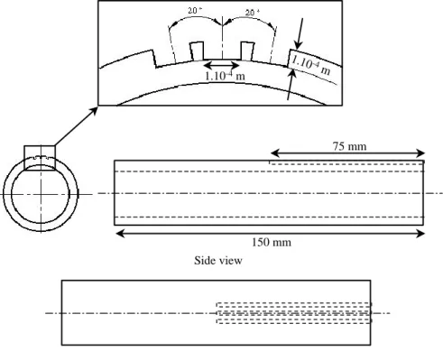
3. PROBE DESCRIPTION

This probe is made out of stainless steel to come under the same thermohydraulic and fouling conditions as heat exchangers. In industrial applications, the inside wall temperature measurement is difficult to accurately check because of noise. With the aim of freeing from this measurement, this probe has two rows of thermocouples in two different radii. The studied probe, 150 mm length, 5 mm inside radius and 11 mm outside radius, can be described by a multilayered system with three concentric cylinders (FIGURE 2). Each stratum is 2 mm thick. In each of the two interfaces between these three cylinders, 10 type T thermocouples distant between them of a 20° angle are stuck. Thus, they are uniformly distributed on a 180° angular sector, the zero corresponding to the stagnation point. Every measurement obtained with these thermocouples is obtained from an average of 60000 points (1 point every 5.10-3 seconds on

300 seconds) to limit errors committed on the measurement. FIGURE 2 HERE

The diameter of the thermocouple hot junction is 1.10-4 meter. The thermocouples are placed

into grooves manufactured straight from the tube (FIGURE 3). All the precautions were taken so that, on one hand, the error committed on the thermocouple locations is as weak as possible (grooves have the same size as hot junction, hot junction was positioned in groove abutment…) and, on the other hand, the contact resistances are as small as possible.

FIGURE 3 HERE The various characteristics of this probe are given on TABLE 1:

It is important to note that a sensitivity study has been realised on the contact resistances between the different layers. This study highlights that the contact resistances have no real impact on the estimation. Moreover, the probe has been calibrated and validated.

4. FORWARD PROBLEM AND INVERSE PROBLEM

In this part, the forward heat transfer problem is presented. It calculates the temperature field inside the sensor. The inverse problem is then examined to allow the determination of the heat transfer coefficient distribution around the probe.

4.1. Forward problem

Internal temperatures of a point P1









known temperature T1 on the internal wall









transfer coefficient varies with the angular abscissa x . The heat transfer coefficient distribution

is supposed symmetric with respect to the plan x0. FIGURE 4 HERE

Temperatures in P1 and in P2 are the solution of the following steady state heat conduction

problem in two dimensions:

 

 

 

The temperature is an even function in x and is periodical with period 2 in x. (2)





_

_

_

_

The cooling water flows through the inner cylinder at a sufficient rate to set its temperature:

 

1 1, 1

rr T r x T (4)

The periodicity and the symmetric conditions relative to the x-coordinate allow us to use the Fourier cosine transform of the temperature:

0

( , ) ( , ) cos( ) with

T r k 



the functions cos kx are the eigenfunctions of the problem in x. The symmetric condition sets

 

In transformed space, the heat equation becomes:

 

 

_{ }

Equation (6) admits for general solution:

 

 

 

where K1, K2, K3, K represent the integration constants. 4

The Fourier cosine transform of the product of the radial heat flux density by the half perimeter can be written:

0 0 ( , ) ( , ) ( , )r k ( , ) cos(r x kx dx) r T r x cos(kx dx) rdT r k r dr           





Thus, the Fourier transform of the boundary condition (3) can be written:

2 2 2 ₀ 2 ₀ 2 2 ( , ) ( , ) ( , )r k ( , ) cos(r x kx dx) r T r x cos(kx dx) r dT r k r dr           









Expressions (6) and (8) are equivalent to a quadrupole presentation (Maillet et. al. 2000). So, the following matrix relationship between the Fourier temperature-flux vectors can be written using this quadrupole formalism for a cylindrical layer rsre thick with r1   re rs r2:

, ( ) ( ) ( ) ( ) ( ) ( ) ( ) ( ) e s e r r s r r k k T k T k k k k k     _                A B C D (11)

with the following values of the coefficients A, B, C, D of the quadrupole matrix defined as:

 

 

 





 

 

 



 



 



 



 



 



It is then possible to define five quadrupole matrices such as:

- M describing the cylindrical layer comprised between the radii ₂ r_e r₀₁ and r_s r₀₂ ; - M describing the cylindrical layer comprised between the radii 3 rer02 and rs r2 ; - M describing the cylindrical layer comprised between the radii ₄ r_e r₀₁ and r_s r₂ ; - M describing the cylindrical layer comprised between the radii r_e r₁ and r_s r₂ ;

Considering that the coefficient subscripts of each matrix are defined by the same way, it is possible to write:













By combining equations (14) and (15), it comes:









By the same way, it is possible to express T_o2 according to T_o1 or according to T₁:

















The inverse Fourier transform (18) allows to calculate T01









2 0 0 if 0 cos( ) ( , ) ( , ) with cos ( ) if 0 2 k k k k kx T r x T r k N kx dx N k           _{ }  



_

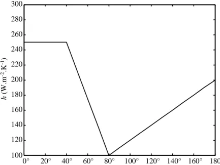
To validate this direct model, a heat transfer coefficient distribution h x representative of

 

crossflow convective cooling of a cylinder in subcritical regime (FIGURE 5) is taken into account (Maillet et. al. 1996):

FIGURE 5 HERE

The temperature distributions obtained from this theoretical heat transfer coefficient distribution are plotted on FIGURE 6. They are calculated from the probe characteristics (Table

1). The temperatures T and ₁ T have been fixed respectively at 283 K and 323 K. _e

FIGURE 6 HERE 4.2. Inverse problem

Now the question is to estimate T₂ and ₂ from the experimental temperature measurements,

01 and 02

T T , in order to obtain the heat transfer coefficient distribution around the probe.

For this, let us consider the matrix M : 2

2 2 01 02 2 2 01 02 T T                    A B C D (19) that involves:

01 2 02 02 2 T T   A B (20)

From matrix M , it comes: 3

02 3 2T 3 2  C D (21) and 02 3 2 2 3 T T   A B (22) By replacing (21) in (22): 2 3 02 3 02 T DT B (23)

So, the expression of T according to ₂ T₀₁ and T₀₂ is obtained by replacing ₀₂ by its value (20) in equation (23): 4 02 3 01 2 2 T T T B B B (24)

And, the expression of ₂ by replacing T by its value ₂ (24) in equation (22):

4 02 3 01 2 2 - T T   A A B (25)

The T₂ and ₂ transforms are calculated harmonic by harmonic from the discret Fourier transform of the temperature measurement at radii r and ₀₁ r . They can also be calculated from ₀₂

these same temperatures calculated from the direct model. Indeed, in both cases, the real values of these temperatures are available. But it is necessary to know them in Fourier space. So:

 

 







where y represents the experimental temperature measurement to an angle x for a fixed _i

radius, and m represents the number of measurements.

Thus, from the T₂ and ₂ inverse Fourier transform (18), it is possible to obtain the estimated heat transfer coefficient angular repartition such as:

 

 

_{ }

The estimation of the angular heat transfer coefficient distribution is realised from experimental noisy temperature measurements. So, the number of harmonics k must be optimised. The optimal value of k is the one that minimises the average temperature residual R between the temperatures calculated from the estimated heat transfer coefficient distribution and the corresponding experimental temperatures:







The average temperature residual value is minimal for a number of harmonics equal to 8. In theory, the spectrum truncation minimises the temperature residuals. In practice, a number of m = 10 temperature measurements are realised. So, it can be possible to evaluate at most k = m harmonics (the number of harmonics k cannot be up to 10) to avoid the aliasing. Besides, the

boundary conditions of such problem involve a soft signal containing a limited number of harmonics.

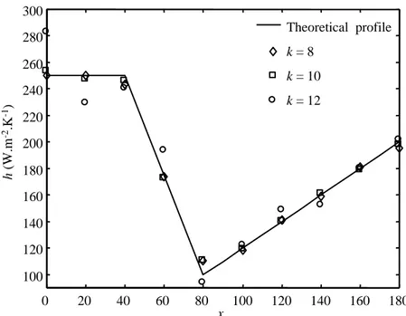
For example, from the calculated temperature distributions at r and at 01 r plotted on 02 FIGURE 6 , it is possible to estimate the heat transfer coefficient distribution plotted on FIGURE 5 for different values of k. It is necessary to notice that for a value of k up to 10, an instability appears for the weak values of x (FIGURE 7).

FIGURE 7 HERE

5. EXPERIMENTAL RESULTS

Thus, thanks to this probe, it seems possible to estimate the angular heat transfer coefficient distribution in clean conditions and the global heat transfer distribution in fouling conditions. 5.1. Experimental results in clean conditions

At first, to confirm the inverse model developed, a set of measurements in clean conditions for different air flow rates was carried out. The air temperature was fixed at 323 K and the different air flow rates were varying from 50 to 100 Nm3.h-1. So, the corresponding Reynolds numbers

calculated from the probe diameter are bounded by 3.103 and 6.103. The temperature responses

obtained from the probe for an 50 Nm3.h-1 air flow rate are presented in FIGURE 8:

FIGURE 8 HERE

The angular heat transfer coefficient distribution has been estimated from these temperature responses and from the detailed inverse method for each air flow rate. Only the results obtained for 50 Nm3.h-1 and 100 Nm3.h-1 air flow rates will be presented in this work.

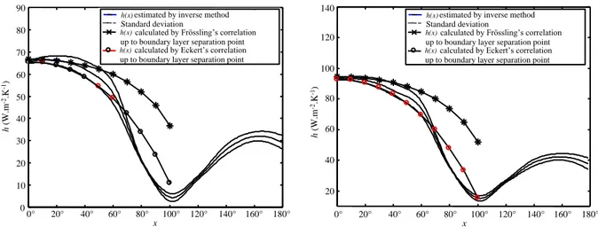
To know if the estimated angular heat transfer coefficient distribution is coherent, two kinds of comparisons are established:

- The first consists in comparing it with other profiles calculated by Eckert’s (Eckert 1942) and Frössling’s (Frössling 1940) correlations applied to our experimental conditions (FIGURE 9):

FIGURE 9 HERE

Experimental data were numerically noise-added with various levels of a white noise in order to calculate the standard deviation of the estimation. The estimated angular heat transfer coefficient repartition is an accurate representation of the heat transfer. Indeed, this heat transfer coefficient is maximal at the stagnation point









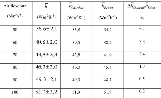
- The second consists in calculating the average heat transfer coefficient from the Churchill’s and the Eckert’s correlations (Churchill 1977; Eckert and Drake 1972) applied to our experimental conditions and from the estimated angular heat transfer coefficient distribution such as:

 

_

Results obtained with this method are presented in TABLE 2: TABLE 2 HERE

The estimated heat transfer coefficient distributions and the average heat transfer coefficients calculated seem to agree with the results obtained by correlations considering the existing distance between these correlations (FIGURE 10).

In conclusion, this probe enables to estimate accurately the angular distribution and the average heat transfer coefficient in clean conditions.

5.2. Experimental results in fouling conditions

The fouling tests were carried out with a duration going from 2 to 72 hours, for an air flow rate of 100 Nm3.h-1 with the air temperature fixed at 353 K. So, the corresponding Reynolds number

calculated from the probe diameter is 5.9.103. The particles dispersion air flow rate is fixed at

6.7.10-8 m3.s-1. The considered fouling durations are too important to highlight the convective

heat transfer coefficient rise when the first layer of the deposit attaches to the surface.

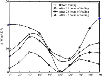
As previously, the inverse method is used. It allows the estimation of the global heat transfer coefficient distribution, which is now a conductance around the probe for various duration of fouling. Indeed, in fouling conditions, the convective heat transfer coefficient becomes a composite coefficient that includes the convective resistance and the fouling resistance. FIGURE

11 represents the conductance distributions for 11 hours, 24 hours and 72 hours of fouling, and the heat transfer coefficient distribution in the same experimental conditions but without injected particles.

FIGURE 11 HERE

The most important local conductance coefficients are situated upstream and dowstream of the cylinder, where the deposit grows the most quickly, respectively by inertial impaction and turbulent projection. For angles comprised between 40° and 140°, this decrease is less important because of a weaker deposit. In fouling conditions, the maximum of the conductance distribution doesn’t take place at the stagnation point but for an angle of 40°. The progressive profilement in droplet shape of the obstacle can explain this phenomenon. Indeed, numerous

the deposit, notably in the neighbourhood of the stagnation point by moving the deposit zone (Fush 1988; Israel and Rosner 1983; Konstandopoulos 1991; Rosner et. al. 1983; Wang 1986; Wessel and Righi 1988). This gap occurs midway between the stagnation point and the boundary layer separation point, typically for angles ranging between 40° and 60°. Thus, the obtained results are in perfect agreement with the bibliographical ones.

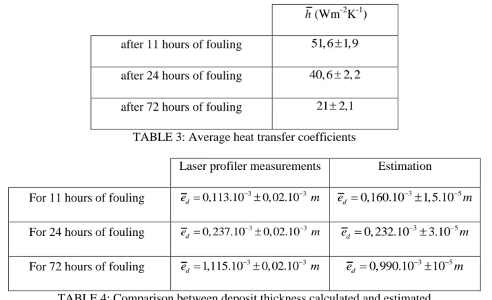
It is also possible to calculate the average heat transfer coefficient (TABLE 3) thanks to these various profiles and from the equation 33:

TABLE 3 HERE

With the aim of quantifying the fouling effects on the heat transfer, the Miller’s parameter of the heat exchange degradation H (Miller 1967) is presented in FIGURE 12. It corresponds to the division of the average conductance in fouling conditions by the average heat transfer coefficient in clean conditions:

 

 

First of all, this heat transfer degradation can be represented by a phase of initiation. Then, it can be represented by a phase of decrease following an exponential law. Indeed, the fouling phenomenon presents generally an asymptotic behaviour which denotes that the fouling resistance reached a limit value. The obtained results are in agreement with the bibliographical ones on the subject. Indeed, it is allowed that in particulate fouling conditions on a tube, there is an asymptotic phenomenon is still not well understood. This phenomenon is attributed either: - to the fact that the profiled tube enters into the flow such as a fine needle by weakly

- or to the fact that there may be a threshold beyond which a balance between the deposit (inertial deposit or turbulent projection deposit) and the re-entrainment associated to the shear and ageing efforts occurs.

So, our probe brings to light this asymptotic phenomenon without however bringing enough dynamic elements on its cause.

The Miller’s parameter can also be expressed from the estimated profiles of the heat transfer coefficient for various duration of fouling. Therefore, it allows to locally quantify the fouling effects on the heat transfer. It is plotted on FIGURE 13.

FIGURE 13 HERE

This parameter is small when the fouling thickness is high as at the stagnation point









- The zone 1 where the organisation of the curves is realised according to the increasing durations of fouling and in which the Miller’s parameter increases until it reaches a threshold. The asymptotic phenomenon is here underlined too.

- The zone 2 corresponds to an abrasion and separation zone. - The zone 3 corresponds to the whirling zone.

A dynamic behaviour where the curves for the different fouling times cross each others is observed in zones 2 and 3. This phenomenon is connected to re-entrainment of the deposit in these zones which are strongly sheared.

inertial impaction and the turbulent diffusion. This comment explains why the measured deposit pattern is not homogeneous around the probe. Every average deposit thicknesses is calculated by integrating these values by the trapeze method.

FIGURE 14 HERE

To check the estimated angular conductance distribution, two kinds of comparisons are established:

- The first (TABLE 4) consists in calculating the average deposit thickness for a fixed fouling duration, from the estimated average coefficients and from the equation (31), and from the

deposit thermal conductivity





The thermal properties of the deposit used here are mean values. They completely disregard of the deposit cohesion which is not homogeneous according to the considered angular position.

TABLE 4 HERE

The deposit thickness values obtained from the estimated average conductances are rather close to the deposit thickness values measured by the laser profiler.

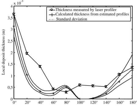
- The second (FIGURE 15) consists in calculating the discrete thickness from the estimated conductance distribution and from the equation (32), then in comparing them with the laser profiler measurements:

 

 

FIGURE 15 HERE

The estimated local deposit thickness around the probe seems to be in good agreement with the deposit thickness measured by the laser profiler. It is important to note that the estimation of the discrete deposit thickness minimises reality for angles lower than 100° and maximises it for angles up to this value. Indeed, calculations were made using a constant value of the deposit thermal conductivity around the tube. In practice, this is not the case: the deposit nature differs according to the deposit regime. Indeed, upstream of the cylinder, deposit is created by inertial impaction, while it is created by turbulent projection downstream. The deposit thermal conductivity considered should be higher upstream of the tube than downstream. So, it would allow to refine results obtained from the estimation of the discrete deposit thickness. Moreover, it is important to notice that equations (31) and (32) does not take into account the fact that, when the first layer of the deposit attaches to the surface, the convective heat transfer coefficient tends to increase due to the increased roughness of the surface.

6. CONCLUSIONS

A thermal probe was designed to be able to replace one part or the totality of heat exchanger tubes. The principle of the method is related to the processing of temperature distributions inside the tube wall. A simple inverse method was implemented in order to estimate the heat exchange coefficient distribution.

The validation of the device was realised in a calibrated environment and the fouling thickness was verified with optical measurements.

This probe has shown its capacity to accurately estimate the heat transfer coefficient profile in clean conditions and the global conductance distribution in fouling conditions, supplying

accurate information on the loss of efficiency of tubular heat exchangers submitted to particulate fouling. The results were successfully confronted with the available data from the literature.

The assets of such a device are the low cost, the convenient data processing and the robustness. The prospects of this work are to extend the method to other exchanger technologies (liquid-liquid, plate heat exchangers,…) and other fouling conditions (corrosion, scaling…). The restrictions of the method are related to the inverse method. A preliminary numerical trial is necessary in order to evaluate the main parameters (number of harmonics as a function of the measurement noise).

7. NOMENCLATURE

Latin letters

, , ,

A B C D Quadrupole coefficients

p

C Constant pressure specific heat J/kg/K -1

L length m

M Quadrupole matrix

N Acquisition points

T Temperature K

e Thickness m

h Convective heat transfer coefficient 2

W/m /K

k Fourier coefficient

r Radial coordinate m

t Time s

x Angular coordinate rad

Greek letters  Flux W  Thermal conductivity W/m/K  _Density 3 kg/m Symbols

Average Fourier transform Subscripts c clean outside e d deposit

8. REFERENCES

(Beal 1970) Beal, S. K. 1970. Deposition of particles in turbulent flow on channel or pipe walls, Nuclear Science and Engineering. (Bott 1992) Bott, T.R. 1992. Heat exchanger fouling. The Challenge.

Fouling Mechanisms : Theorical and Practical Aspects,

Eurotherm Seminar 23, 3-10, Grenoble, France.

(Bouris and Bergeles 1996) Bouris, D., Bergeles, G. 1996. Particle-Surface Interactions in Heat Exchanger Fouling, Journal of Fluids Engineering, 118:574-581.

(Churchill 1977) Churchill, S. W., Bernstein, M. 1977. A correlating equation for forced convection from gases and liquids to a circular cylinder in crossflow, Journal of Heat Transfer, ASME 99:300-306.

(Eckert 1942) Eckert, E. R. 1942. Die Berechnung des Wärmeüberganges in der laminaren Grenzschicht umströmter Körper,

VDI-Forschungsheft:416.

(Eckert and Drake 1972) Eckert, E. R., Drake, R. M. 1972. Analysis of heat and mass transfer, Mac Graw-Hill, New York.

(Epstein 1978) Epstein, N. 1978. Fouling in heat exchangers, Heat Transfer 1978 : 6th International Heat Transfer Conference, 6, 235-253.

(Finkbeiner et. al. 1993) (In French) Finkbeiner, F., Gonard, T. and Filiol, B. 1993.

politique d’innovation., (Heat exchangers, Wagers, technology and innovation politic) Editions européennes

Thermique et Industrie (EETI), France.

(Frössling 1940) Frössling, N. 1940. Verdunstung, Wärmeübergang und Geschwindigkeitsverteilung bei zweidimensionaler und rotationasymmetrischer Grenzschichtströmung, Lunds Univ Arsskr Avd 2, 36:4.

(Fush 1988) Fush, S. E. 1988. Studies of inertial deposition of particles onto heat exchanger elements, PhD Thesis, California Institute of Technology.

(Glen and Howarth 1988) Glen, N. F., Howarth, J. H. 1988. Modelling refuse incineration fouling, 2nd United Kingdom Conference on Heat Transfer, Institute of Mechanical Engineering, 1:401-

420.

(Israel and Rosner 1983) Israel, R., Rosner, D. E. 1983. Use of a generalized Stokes number to determine the aerodynamic capture efficiency of non-Stokesian particles from a compressible gas-flow,

Journal of Aerosol Science and Technology, 2:45-51.

(Kern and Seaton 1959) Kern, D.Q., Seaton, R.E. 1959. A theoretical analysis of thermal surface fouling., Britanic Chemical Sciences 4, 5:258-262.

(Konstandopoulos 1991) Konstandopoulos, A. G. 1991. Effects of particle inertia on aerosol transport and deposit growth dynamics. PhD Thesis, Yale University, New Haven.

(Louahlia-Gualous et. al. 2002) Louahlia-Gualous, H., Artioukhine, E., Panday, P. K. 2002. The inverse estimation of the local thermal boundary conditions in two dimensional heated cylinder, 4th

International Conference on Inverse Problems in Engineering, Rio de Janeiro, Brazil.

(Maillet and Degiovanni 1989) (In French) Maillet, D., Degiovanni, A. 1989. Méthode analytique de conduction inverse appliquée à la mesure du coefficient de transfert local sur un cylindre en convection forcée, ( Inverse heat conduction analytical method applied to the measurement of the local heat transfer coefficient on a cylinder in forced convection) Revue de physique

Appliquée, 24:741-759.

(Maillet et. al. 1996) Maillet, D., Degiovanni, A., André, S., 1996, Estimation of a space varying heat transfer coefficient or interface resistance by inverse conduction. Proceeding 23rd

International Thermal Conduction Conference, K. E. Wilkes, R. B. Dinwiddie and R. S. Graves editions, Nashville, 29 October – 1 november, Technomic Publishers Co. Lancaster, 72-84.

(Maillet et. al. 2000) Maillet, D., André, S., Batsale, J. C., Degiovanni, A., Moyne, C. 2000. Thermal quadrupoles, solving the heat equation through integral transforms, Editions Wiley and Sons.

(Marner 1990) Marner, W. J. 1990. Progress in gas-side fouling of heat transfer surfaces, Applied Mechanical Revue, 43: 35-66. (Martin and Dulikravich 1998) Martin, T. J., Dulikravich, G. S. 1998. Inverse

determination of steady heat convection coefficient distributions, Transactions of the ASME, 120: 328-334. (Miller 1967) Miller, J.A. 1967. Mechanisms of gas turbine regenerator

fouling, n°67-LGT-26, ASME, New York.

(Pasquetti et. al. 1991) Pasquetti, R., Maillet, D., Degiovanni, A. 1991. Inverse heat conduction applied to the measurement of heat transfer coefficient on a cylinder : comparison between an analytical and a boundary element technique, Journal of Heat

Transfer, 113: 549 – 557.

(Rosner et. al. 1983) Rosner, D. E., Gokoglu, S. A., Israel, R. 1983. Rational engineering correlations of diffusional and inertial particle deposition behaviour in non-isothermal forced convection environments, Fouling of heat exchanger surfaces, 235-256. (Sheikh et. al. 2000) Sheikh, A. K., Zubair, S. M., Younas, M., Budair, M. O.,

2000. A risk based heat exchanger analysis subject to fouling : Economics of heat exchangers cleaning, Energy 25, Elsevier Editions, 445-461.

(Sullivan et. al. 2002) Sullivan, G. P., Hunt, W. D., Melendez, A. P., Pugh, R. 2002. Operations and maintenance, Best practices, A guide to achieving operational efficiency, US Department of

Energy.

(Taborek et. al. 1979) Taborek, J., Aoki, T., Ritter, R. B., Palen, J. W. 1979. Fouling : The major unresolved problem in heat transfer,

Chemical Engineering Process, 68(2):59-67.

(Thomas and Grigull 1974) Thomas, D., Grigull, U. 1974. Experimental investigation of the deposition of suspended magnetite from the fluid flow in steam generating boiler tubes, Brennst-Warme Kraft, 109-115.

(Wessel and Righi 1988) Wessel, R. A., Righi, J. 1988. Generalized correlations for inertial impaction of particles on a circular cylinder, Journal

of Aerosol Science and Technology, 9: 20-60.

(Wang 1986) Wang, H. C. 1986. Theoretical adhesion efficiency for particles impacting a cylinder at high Reynolds number,

Journal of Aerosol Science and Technology, 17: 827-837.

(Watkinson and Epstein 1970) Watkinson, A. P., Epstein, N. 1970. Particulate fouling of sensible heat exchangers, 4th International Heat Transfer Conference, 1:1-12.

Air with particles Cooling water Air at 343 K Foulant particles generator Heat exchanger parts

and probe Industrial water sewer Air with particles Cooling water Air at 343 K Foulant particles generator Heat exchanger parts

and probe

Industrial water

sewer

FIGURE 1: Experimental testing device GAZPAR

02 r 1 r r01 r2 thermocouples 20° 0 x  180 x 

Top view Side view 1.10-4 _m 1.10_-4 m 75 mm 150 mm

FIGURE 3: Simplified scheme of one tube of the probe

02 r 1 r r01 r2 e T 1 T r

 

0° 20° 40° 60° 80° 100° 120° 140° 160° 180° 100 120 140 160 180 200 220 240 260 280 300 h ( W .m -2.K -1) x

FIGURE 5: Theoretical heat transfer coefficient distribution

0° 20° 40° 60° 80° 100° 120° 140° 160° 180° 13 14 15 16 17 18 19 20 Te m per at ure s a t r adi i r01 a nd r 02 ( °C ) x 01 T 02 T

h (W.m -2.K -1) x 0 20 40 60 80 100 120 140 160 180 100 120 140 160 180 200 220 240 260 280 300 Theoretical profile k = 8 k = 10 k = 12

FIGURE 7: Heat transfer coefficient profiles estimated for different values of k

10,5 11 11,5 12 12,5 13 13,5 Experimental temperatures y Experimental temperatures y 01 at r 02 at r 01 02 0° 20° 40° 60° 80° 100° 120° 140° 160° 180° x Ex pe ri me nta l te mpe ra tur es ( °C)

0 10 20 30 40 50 60 70 80 90 0° 20° 40° 60° 80° 100° 120° 140° 160° 180° x h ( W .m -2.K -1)

h(x) estimated by inverse method Standard deviation

h(x) calculated by Frössling’s correlation up to boundary layer separation point

h(x) calculated by Eckert’s correlation up to boundary layer separation point

0° 20° 40° 60° 80° 100° 120° 140° 160° 180° x h (W .m -2.K -1) 20 40 60 80 100 120 140

h(x) estimated by inverse method Standard deviation

h(x) calculated by Frössling’s correlation up to boundary layer separation point

h(x) calculated by Eckert’s correlation up to boundary layer separation point

for 50 Nm3/h air flow rate for 100 Nm3/h air flow rate

FIGURE 9: Comparisons between h(x) profiles estimated and calculated by correlations

50 55 60 65 70 75 80 85 90 95 100 30 35 40 45 50 55 60

Average heat transfer coefficient obtained by inverse method Average heat transfer coefficient obtained by Churchill’s correlation

Average heat transfer coefficient obtained by Eckert’s correlation

h

(W.m

-2.K -1)

Air flow rate (Nm3_.h-1₎

FIGURE 10: Comparisons between heat transfer coefficient average values obtained by calculation and by correlations

x 0° 20° 40° 60° 80° 100° 120° 140° 160° 180° 0 50 100 150 Before fouling After 11 hours of fouling After 24 hours of fouling After 72 hours of fouling

h

(W

.m

-2.K -1)

FIGURE 11: Estimated profiles of the thermal conductance for various durations of fouling

0 10 20 30 40 50 60 70 80 0,3 0,4 0,5 0,6 0,7 0,8 0,9 1 Duration (hours) H Phase of initiation Phase of decrease

0° 20° 40° 60° 80° 100° 120° 140° 160° 180° 0 0,2 0,4 0,6 0,8 1 H in clean conditions

H after 11 hours of fouling

H after 24 hours of fouling

H after 72 hours of fouling

H

x

1 2 3

FIGURE 13: Local heat transfer degradation represented by Miller’s parameter

Air flow direction

Air flow direction

Deposit pattern after 11 hours of fouling Deposit pattern after 24 hours of fouling

3 3 0,113.10 0, 02.10 d e     m e_d 0, 237.1030, 02.10 3 m Air flow direction

Deposit pattern after 72 hours of fouling

3 3

1,115.10 0, 02.10

d

-3 0° 20° 40° 60° 80° 100° 120° 140° 160° 180° 0 0,5 1 1,5 2 2,5 3 3,5 4x 10 x Loc al de posi t t hi ckne ss ( m )

Calculated thickness from estimated profiles Standard deviation

Thickness measured by laser profiler

FIGURE 15: Comparison between local thickness measured by the laser profiler and calculated from the estimated heat transfer and conductance profiles for 72 hours of fouling

Dimensions inside radius r15 mm 1st radius of measurement r017 mm 2nd radius of measurement r029 mm outside radius r2 11 mm length L150 mm ther mal pr ope rties

stainless steel thermal conductivity

-1 1 16,3 W.m .K

_ 

stainless steel heat capacity Cp 4.10 J.m .6 -3K 1

 

TABLE 1: Probe characteristics

Air flow rate (Nm3h-1) h (Wm-2K-1) Churchill h (Wm-2K-1) ker Ec t h (Wm-2K-1) ker Churchill Ec t h h  % 50 36, 6 2,1 35,8 34,2 4,7 60 40, 6 2, 0 39,5 38,2 3,3 70 43,9 2,3 42,8 41,9 2,4 80 46,3 2, 0 46,0 45,4 1,3 90 49,3 2,1 49,0 48,7 0,5 100 52, 7 2, 2 51,9 51,9 0,2

TABLE 2: Comparisons between heat transfer coefficient average values estimated from the measurements and calculated by correlations

h(Wm-2K-1) after 11 hours of fouling 51, 6 1,9 after 24 hours of fouling 40, 6 2, 2 after 72 hours of fouling 21 2,1

TABLE 3: Average heat transfer coefficients

Laser profiler measurements Estimation

For 11 hours of fouling e_d 0,113.1030, 02.10 3 m e_d 0,160.1031,5.105m

For 24 hours of fouling e_d 0, 237.1030, 02.10 3 m e_d 0, 232.1033.105m

For 72 hours of fouling ed 1,115.103 0, 02.10 3 m

 

  3 5

0,990.10 10

d

e     m