HAL Id: halshs-00564865
https://halshs.archives-ouvertes.fr/halshs-00564865
Preprint submitted on 10 Feb 2011
HAL is a multi-disciplinary open access
archive for the deposit and dissemination of
sci-entific research documents, whether they are
pub-lished or not. The documents may come from
teaching and research institutions in France or
L’archive ouverte pluridisciplinaire HAL, est
destinée au dépôt et à la diffusion de documents
scientifiques de niveau recherche, publiés ou non,
émanant des établissements d’enseignement et de
recherche français ou étrangers, des laboratoires
Survival, reproduction and congestion: The spaceship
problem re-examined
Pierre-André Jouvet, Grégory Ponthière
To cite this version:
Pierre-André Jouvet, Grégory Ponthière. Survival, reproduction and congestion: The spaceship
prob-lem re-examined. 2010. �halshs-00564865�
WORKING PAPER N° 2010 - 15
Survival, reproduction and congestion:
The spaceship problem re-examined
Pierre-André Jouvet
Grégory Ponthière
JEL Codes: D63, Q56, Q57
Keywords: environmental congestion, fertility, longevity,
population ethics, utilitarianism, renewal
P
ARIS
-
JOURDAN
S
CIENCES
E
CONOMIQUES
48,BD JOURDAN –E.N.S.–75014PARIS TÉL. :33(0)143136300 – FAX :33(0)143136310
www.pse.ens.fr
CENTRE NATIONAL DE LA RECHERCHE SCIENTIFIQUE –ECOLE DES HAUTES ETUDES EN SCIENCES SOCIALES
Survival, reproduction and congestion:
the spaceship problem re-examined
Pierre-André Jouvet and Gregory Ponthiere
yApril 28, 2010
Abstract
This paper re-examines the spaceship problem, i.e. the design of the optimal population under a …xed living space, by focusing on the dilemma between adding new beings and extending the life of existing beings. For that purpose, we characterize, under time-additive individual welfare de-pending negatively on population density, the preference ordering of a utilitarian social planner over lifetime-equal histories, i.e. histories with demographic conditions yielding an equal …nite number of life-periods (im-posed by resources constraints). The analysis of the spaceship problem contradicts widespread beliefs about the populationism of Classical Util-itarianism and the antipopulationism of Average UtilUtil-itarianism. We also study the invariance property exhibited by various utilitarian rankings to the total space available and to individual preferences. Finally, we com-pare histories for a spaceship with a stationary population, and try to accomodate intuitions about posterity and renewal of populations.
Keywords: environmental congestion, fertility, longevity, population ethics, utilitarianism, renewal.
JEL codes: D63, Q56, Q57.
EconomiX, University Paris-Ouest, Nanterre - La Défense, and CORE. Address: Univer-sity Paris-Ouest, 200, avenue de la République, building K and G, 92001 Nanterre, France.
yParis School of Economics and Ecole Normale Supérieure, Paris [corresponding author].
Address: Ecole Normale Supérieure, Department of Social Sciences, boulevard Jourdan, 48, building B, 75014 Paris, France. E-mail: gregory.ponthiere@ens.fr Telephone: 0033-1-43-13-62-04. Fax: 0033-1-43-13-62-22.
1
Introduction
Given that the Earth is of …nite size - and, thus, can be compared, following Boulding (1966), to a ‘spaceship’- the question of the optimal population size can be formulated as the ‘spaceship problem’: are there too few or, on the contrary, too many beings living on our bounded, resources-…nite, spaceship? That question, which is today at the centre of sustainable development debates, is actually an old issue, to which various answers were given over time.
While Mercantilism was, during the 16th and 17th centuries, promoting a population as large as possible by means of various policies, it should not be deduced from this that the spaceship constraint was ignored by Mercantilist thought.1 Actually, it is quite the opposite: a standard Mercantilist argument
was that the …niteness of the living space, if coupled with a large population, would favour migrations, and, hence, the colonization of other territories.
The Italian philosopher Giovanni Botero (1588) is generally regarded as one of the …rst thinkers who argued against the Mercantilist populationism, and asked the question of the optimal population size. Botero argued that men have a tendency to multiply themselves as much as nature allows. However, natural resources are limited, so that, according to Botero, one cannot escape the following adjustments: either people will modify their behaviours, or there will be some adjustment in numbers through famines, diseases or wars.
Within economic thought, Richard Cantillon (1755) provided another early study of the spaceship problem, by highlighting the existence of a quantity of life versus quality of life trade-o¤, which restrains feasible population sizes. According to Cantillon, Man’s subsistence requires living space, whose amount depends on lifestyles, so that an arbitrage is to be made between the quantity and quality of life.2 While Cantillon did not solve that trade-o¤, he showed
that, contrary to Mercantilists’beliefs, more people is not always better.3
Another contribution to the spaceship problem was made by Thomas Malthus (1798), who argued that the population size is necessarily limited within some boundaries. A population would follow a geometric progression if left unchecked (i.e. in the absence of resources constraints), but the production of means of subsistence follows, at best, an arithmetical progression (because of the …nite-ness of land), so that the population must, at some point, be ‘checked’, either by a positive check (deaths) or by a preventive check (fewer children).4
Given that Botero, Cantillon and Malthus’s positive theories, by underlining the constraints imposed by the …niteness of land, only restrict the set of feasible populations, these leave open the normative question of the optimal population. That issue was widely studied within utilitarianism. While Jeremy Ben-tham’s (1789) Classical Utilitarianism recommends a number of people produc-ing ‘the greatest happiness of the greatest number’, one may also, followproduc-ing
1On Mercantilism and population, see Schumpeter (1954, 1, pp. 352-356).
2See Cantillon’s comparison of peasants living modestly in the South of France with
grown-up bourgeois living in abundance (1755, p. 25).
3See Cantillon (1755, I, 15, p. 30):
‘It is also a question outside of my sub ject whether it is better to have a great multitude of inhabitants, poor and badly provided, than a small number, much more at their ease: a million who consume the produce of 6 acres per head or 4 million who live on the product of an acre and a half.’
Sidgwick’s (1874) insights, consider the maximization not of total welfare, but of average welfare, which di¤ers from Benthamite utilitarianism in di¤erent numbers choices. However, as shown by Par…t (1984), those two criteria of population ethics are unsatisfactory. Classical Utilitarianism su¤ers from the Repugnant Conclusion, whereas Average Utilitarianism faces the Mere Addi-tion Paradox.5 Hence, other population ethics criteria were developed, such as Critical-Level Utilitarianism (Blackorby and Donaldson 1984) and Number-Dampened Utilitarianism (Ng 1986). But although (partly) immunized against Par…t’s criticisms, these su¤er from other weaknesses. Imposing a low critical level still implies the Repugnant Conclusion, while a high critical level leads to what Arrhenius and Bykvist (1995) call the Sadistic Conclusion.6 Moreover,
Number-Dampened Utilitarianism might lack intuitive support.
Although much has been written on the optimal population of the Earth spaceship, the speci…city of this paper with respect to the existing literature is precisely to consider the spaceship problem on the basis of new fundamentals. Actually, instead of studying the optimal population size without specifying the structure of the population, we propose to re-examine that issue under a more precise speci…cation of the populations at stake. For that purpose, we will distinguish here between the two ends of the demographic ‘chain’: births and deaths. The intuition is the following. As stressed by Broome (2004), the issue of the optimal number of people is not independent from the issue of the optimal longevity. True, making a person exist and making an existing person live more are, from a moral point of view, two distinct things, but these tend both to in‡uence the number of people at a given point in time, so that the two ends of the demographic chain are relevant for the spaceship problem.
Therefore, we propose a re-examination, from a utilitarian perspective, of the spaceship problem, in which both reproduction and survival are explicitly modelized. The question raised is the following. Suppose that a population, which cares about living a long life in a large living space, has to share a space of …nite size. How does the optimal population look in terms of fertility rate and longevity? To answer that question, we will make some signi…cant simpli…ca-tions, so that the present study should only be regarded as a …rst step towards a characterization of the solution of the spaceship problem.
First, in order to formalize the longevity versus fertility trade-o¤s, we will characterize the preferences of a social planner over lifetime-equal histories, de…ned by demographic conditions (i.e. initial population, fertility and survival rates) yielding an equal …nite number of life-periods.7 The intuition behind assuming a …nite length of history is that some constraints, such as a given stock of non-renewable resources, may tend to limit the total number of periods that can be collectively lived on the spaceship. However, in the last part of the paper we relax that assumption and focus on a spaceship with a stationary
5The Repugnant Conclusion is de…ned as follows: for any large population, there is a much
larger population with a much lower welfare per head, but which is regarded as better. The Mere Addition Paradox consists of regarding as undesirable the addition of people with a welfare slightly lower than the initial average welfare, even if the welfare of the initial popula-tion is una¤ected. Average Utilitarianism violates the Mere Addipopula-tion Principle, according to which adding persons with a positive welfare should not make things worse ceteris paribus.
6The Sadistic Conclusion consists of preferring a small population with an extremely low
utility to a very large population just below the critical level (see Bykvist 2007).
7Reasoning under a …xed total number of life-periods is an analytically convenient way to
population. That latter case coincides with an in…nite history.
Moreover, this paper will not consider here the question of the optimal di-versity of the population to be put on the spaceship, contrary to the literature dedicated to the Noah’s Ark Problem (see Weitzman 1998). On the contrary, we will, in this paper, focus on the characterization of the population that yields the maximum welfare under a uniform composition of that population.
Furthermore, in our model, the numbers’s pressure comes only from popula-tion density, which reduces welfare through a pure congespopula-tion e¤ect (see Cramer et al 2004). Thus, we will not study here the production of goods, which, since Malthus’s work, has occupied a central place in the spaceship problem. Given the observed growth of production per head despite the large population growth, production limitations due to the …niteness of land do not seem likely.8
Finally, given the intuitive weaknesses faced by various criteria of population ethics (see Blackorby et al 2005), it makes sense to re-examine the spaceship problem on the basis of several ethical criteria. However, due to space con-straints, we shall here focus only on some widely used normative criteria, such as Classical, Average, Critical-Level and Number-Dampened Utilitarianisms, and leave other criteria aside, which is also a signi…cant simpli…cation.
The paper is organized as follows. Section 2 introduces our framework. Section 3 studies a simpli…ed spaceship problem, in which the population cannot reproduce itself, and characterizes the ordering of lifetime-equal histories under various utilitarian criteria. Section 4 explores the more general problem where the population can reproduce itself. Section 5 considers a stationary spaceship (i.e. with a constant asymptotic population). Section 6 concludes.
2
The spaceship problem: general setting
The spaceship problem consists of the choice of a population to be put on a spaceship, that is, a place with a …nite surface for life. By the terms ‘choos-ing a population’, we mean the choice of not only an initial group of people (i.e. the ‘pioneers’) to be put on the spaceship, but, also, the choice of survival conditions for them, as individual longevity is, given the …niteness of the space-ship, a¤ected by the size of the group of pioneers. Congestion is not neutral for longevity, because overpopulation can prevent the access to vital resources (through depletion, pollution or other phenomena). Thus, depending on the more or less large initial size of the group of pioneers, each pioneer will have, given the …niteness of the spaceship, a more or less short life.
Examples of spaceship problems are numerous. One can consider the selec-tion of an optimal number of astronauts to be sent into space on a rocket. In that case, there will be, in general, no opportunity for astronauts to reproduce themselves in the spaceship, so that survival conditions depend exclusively on the size of the initial group. Another example of a spaceship problem consists of the selection of a population to live on a planet. In that case, survival conditions depend on the size of the initial group, but there is a di¤erence with respect
8Actually, as Heilig (1994) argues in the light of (mistaken) past studies on the maximum
carrying capacity of the Earth in terms of population, the …niteness of space does not seem to be a problem for production, so that we can abstract from that constraint. One may go further, and argue, following Kremer (1994), that population pressure is good for production, as technological progress is proportional to the population size.
to the rocket case: the general living conditions on the planet may allow the reproduction of persons, so that survival conditions depend also on the fertility behaviour, which may cause shorter lives through environmental congestion.
2.1
Assumptions
Before examining those various kinds of spaceship problems in more detail, let us …rst formally introduce the general spaceship problem and the assumptions that we will make throughout this paper.
Assumption A1 A place of …nite surface Q is available for the life of a population.
Assumption A2Only living persons occupy a part of the space Q. Moreover, all living persons at a particular point in time t = 0; 1; 2; :::; 1, whatever their age is, are assumed to occupy an equal amount of space, de…ned as the total space divided by the number of people alive at that time.9
Assumption A3Each person alive at time t enjoys an equal share of the total available space: qt = LQt, where Lt denotes the population size at
time t, whereas qt denotes the space available per person.
Here are the assumptions we make on individual welfare.
Assumption A4At each period, the temporal welfare of a person who is dead equals 0:
ut= 0 8t T
where T denotes the date of death of the person.
Assumption A5At each period, the temporal welfare of a person who is alive depends on the space available per person, according to the function:
ut= u(qt) = (qt) + 8t < T
where 0 < < 1 and is the intercept of the temporal utility function. Assumption A4 is a standard normalization.10 Assumption A5 is a simple
way to capture the disutility from environmental congestion due to overpopula-tion. According to A5, adding one person to a spaceship of …nite size necessarily decreases the welfare of every individual on the spaceship.11 Note that, if 0,
being alive is always better than being dead, whatever the level of qt is. On
the contrary, if < 0, there exists a level of qtthat makes a person indi¤erent
between, on the one hand, one life-period with that space, and, on the other hand, being dead during that period.
9Thus we will abstract here from problems of intragenerational distribution of space. 1 0A4 allows us also to avoid di¢ culties associated with the possibility of in…nite utility,
which would occur under a non-zero utility of death, as dead persons remain dead in…nitely.
1 1In reality, it is only below some threshold for q
tthat adding one person reduces the welfare
Assumption A6 The lifetime welfare w of a person is the sum of the utilities associated to each life-period:
w =
T
X
t=0
u (qt)
Assumption A6 is, although largely questioned by Bommier (2006), still a standard one, due to its simplicity. Let us now turn to the characterization of the demography.
Assumption A7 The initial population of the spaceship, denoted by L, is …nite and strictly positive (L > 0).
Assumption A8At each passage of time, a fraction S of the population alive at a period survives to the next period (0 < S < 1).
Assumption A8 amounts to assuming that the strength of mortality is con-stant over the lifecycle: at each passage of time, a concon-stant fraction of a cohort disappears from the spaceship. Assumption A8 is made to restrict the longevity dimension to a single parameter, S.
Assumption A9A person surviving to the second period of life will give birth to n children at the beginning of that second period (n 0). Assumption A9 amounts to supposing that the ‘intensity of desires’ (in Malthus’s words) or the need for a dynasty is constant across people and times.12
This allows us to con…ne fertility concerns to a single parameter, n.13
2.2
Problem setting
In order to study how a social planner solves the spaceship problem, de…ned as the choice of an initial number of persons L, a proportion of survivors S, and a fertility rate n under the space constraint, we assume that the social planner has to choose among a set of histories, de…ned as follows.
De…nition D1A history is a triplet fL; S; ng, where L is the size of the population at time 0 (L > 0), S is the proportion of survivors from a period t to a period t + 1 (0 < S < 1), and n is the fertility rate.
In order to describe the planner’s solution, we shall concentrate on a partic-ular subset of the set of histories: lifetime-equal histories, de…ned as follows.14
1 2A9 amounts to assuming that all births are located, for a given person, during, and only
during, the second period of his life, and, more exactly, at the beginning of that second period. For instance, the S2Lmembers of cohort 0 who are alive in their third period of life do not give birth to any o¤spring in period 2 and beyond, but only at the beginning of period 1, and the utility of their children is counted for the whole period during which they are born.
1 3Note that this model does not distinguish between males and females, so that n, the
fertility rate per person, concerns all people, and not only women as in real life. A fertility rate of 2 children per women would correspond to n = 1 in this model.
1 4To be precise, lifetime-equal histories mean total lifetime-equal histories, in the sense that
it is the total sum of the lifetimes of all agents that is equal across histories. In the rest of the paper, we will use the term ‘lifetime-equal histories’ for short.
De…nition D2Two histories fL; S; ng and f ~L; ~S; ~ng are lifetime-equal if and only if these exhibit an equal total number of life-periods.
Note that the total number of life-periods for the …rst cohort (i.e. the pio-neers), denoted by P0, is15
P0= L + SL + S2L + ::: = L
1 1 S
The total number of life-periods for the second cohort, denoted by P1, is
P1= SLn + S2Ln + S3Ln + ::: = LSn
1
1 S
One can then de…ne the total number of life-periods for all other cohorts, denoted by P2, P3, ... etc. The total number of life-periods for a cohort j is
Pj = LnjSj
1
1 S
Hence the total number of life-periods, denoted by P , is P = 1 X t=0 Pt= L 1 1 S 1 + nS + n 2S2+ :::
Note that P is in…nite if nS 1. However, for nS < 1, we have
P = L
(1 S)(1 nS) That ratio can be decomposed in two factors: 1
1 S is the average longevity
for any person, that is, the inverse of the strength of mortality, whereas L 1 nS is
the total number of persons ever born: it is the product of the initial population size L and the strength of fertility 1 nS1 (i.e. the average number of descendants for each person in the initial population). Thus the product of those two factors
1 1 S and
L
1 nS yields the total number of life-periods P .
Note that the total number of life-periods is increasing in the initial popu-lation size L (i.e. @P@L > 0), increasing in the survival rate S (i.e. @P@S > 0), and also increasing in the fertility rate n (@P@n > 0).
In order to remain within the …eld of …nite ethics, we will, in Sections 3 and 4, concentrate on the case where nS < 1, guaranteeing a …nite total number of life-periods, that is, a mankind history of …nite length.16
Assumption A10Only a …nite number of life-periods will be lived on the spaceship: nS < 1.
Assumption A10 can be regarded as a constraint resulting from the …niteness of, let us say, the stock of some non-renewable natural resources present on
1 5In this paper, we mean, by a ‘life-period’, a ‘period lived by someone’. For instance, if
two persons live one period, we say that the total number of life-periods equals two.
the spaceship.17 Under A10, we focus on lifetime-equal histories fL; S; ng and
f ~L; ~S; ~ng, which, by de…nition, are such that: L
(1 S)(1 nS) =
~ L (1 S)(1~ ~n ~S)
For a given number of pioneers (i.e. L = ~L), an equal number of life-periods (i.e. P = ~P ) means that if one lifetime-equal history exhibits a higher fertility n than another one, it must also exhibit a lower survival rate S.
Whereas the comparison of lifetime-equal histories fL; S; ng and f ~L; ~S; ~ng can take various forms, we will start with the simple case where there is no possibility for the initial population to reproduce itself (i.e. n = ~n = 0). Then, in a second stage, we will consider the case where reproduction exists, so that new people can appear at each point in time (n > 0 and nS < 1). Finally, we will turn to the case where nS = 1, which yields an in…nite number of periods lived by a population, whose size converges asymptotically towards some constant.
3
The spaceship problem (1): no reproduction
This section examines a simpli…ed version of the spaceship problem, in which the population cannot reproduce itself. That subcase of the spaceship problem will be referred to as the spaceship problem without reproduction. The absence of reproduction amounts to assuming the following.
Assumption A11The fertility rate n is equal to 0.
Under A11, all new people are concentrated on the …rst period, t = 0, and form the initial population L of …nite size. The total number of periods P lived by a population of initial size L is:
P = L + SL + S2L + ::: = L 1
1 S
Thus, if S tends towards 0, P tends towards L: the number of life-periods equals the number of persons. However, if S tends towards 1, P tends towards +1: as there is no death, the number of life-periods is in…nite.18
Hence, in the spaceship problem without reproduction, comparing two lifetime-equal histories fL; S; 0g and f ~L; ~S; 0g amounts to comparing two histories for which:
1 7Note that assuming nS < 1 yields a total population at time t that converges
asymptoti-cally towards 0. Indeed, writing Ltthe number of people alive at time t, we have
L1= lim
t!1Lt= LS
1+ (LSn)S1 1+ (LS2n2)S1 2+ ::: + L(S1n1)Sn = 0
as S < 1. Thus, our spaceship will, under nS < 1, end up empty in the long-run. But this asymptotic emptyness does not prevent a temporary growth of the spaceship population: the only thing that it prevents is a permanent growth or a stationary positive size.
1 8It follows from the previous formulae that, if S tends to 1, the space available per person
qtis constant over time and equal to Q=L, as: limS!1qt= limS!1SQtL =
Q
L. In that case,
the population that is alive initially will remain forever in the spaceship, and will enjoy the same space conditions during their whole life. On the contrary, if S tends towards 0, qttends
to be in…nite for any t > 0, as: limS!0qt = limS!0SQtL = Q
0 = +1. Indeed, as S tends
L 1 1 S = ~L
1 1 S~ which can be rewritten:
L ~ L =
1 S
1 S~
that is, there is an equality of the ratios of initial populations (LHS) and strengths of mortality (RHS) for histories fL; S; 0g and f ~L; ~S; 0g having an equal number of life-periods. If one history exhibits a larger initial population than another history with the same total number of life-periods (i.e. L > ~L), it must also be characterized by a larger mortality (i.e. 1 S > 1 S).~
3.1
The Classical Utilitarian solution
According to Classical Utilitarianism (CU), as …rstly stated by Bentham (1789), all actions - at the individual and institutional levels - should be chosen in such a way as to produce the ‘greatest happiness of the greatest number’, in conformity with the Principle of Utility. That principle must also govern the choice of histories in general, and, in particular, of lifetime-equal histories.19
De…nition D3A social planner is Classical Utilitarian (CU) if and only if, when facing two histories fL; S; ng and f ~L; ~S; ~ng, he prefers the history yielding the highest total welfare, that is,
fL; S; ng f ~L; ~S; ~ng ()P1t=0Ltu(qt) P1t=0L~tu(~qt)
Regarding the preferences of a CU social planner over lifetime-equal histo-ries, Proposition 1 states a general result: a CU social planner prefers lifetime-equal histories with the smallest population size and the largest life expectancy. Proposition 1 Assume A1-A11. Consider two lifetime-equal histories fL; S; 0g and f ~L; ~S; 0g, with L > ~L and S < ~S. A CU planner prefers f ~L; ~S; 0g to fL; S; 0g, whatever the levels of Q, and .
Proof. See the Appendix.
The result stated in Proposition 1 is quite surprising, as the existing litera-ture on normative population ethics has, since Par…t’s (1984) Repugnant Con-clusion, highlighted the tendency of CU to lead to excessively large populations with low levels of utility per person, a recommendation regarded as ‘repugnant’ by many theorists. On the contrary, Proposition 1 states that, when facing a choice between lifetime-equal histories, CU selects the history with the smallest population. We are thus far from the populationism associated with CU.
While a proof of Proposition 1 is provided in the Appendix, we can give here some intuition behind CU’s preference for small populations.20 Actually, if one
computes the marginal social welfare gain from raising L while maintaining the
1 9Note that the Benthamite ob jective function does not involve any discounting here, in
conformity with Ramsey’s (1928) views. Note also that the above formula presents social welfare by aggregating across time periods rather than persons (as usually done), but this is equivalent to aggregating across people, because of the additivity of lifetime welfare.
2 0It should be stressed here that Assumption A5 is a major driving force for that result. If
we added, instead of A5, temporal welfare invariant to qt above some threshold of qt, then
total number of life-periods L=(1 S) constant, one can see that such a marginal social welfare gain is, under CU, necessarily negative.21 Thus adding one more
being while reducing the expected lifetime of all existing beings in such a way as to maintain total lifetime constant is welfare-reducing under CU.
Note also that Proposition is quite general, as this holds whatever the total space Q is, and for all values of preference parameters and . That latter point is surprising, as we would expect to matter for choices between alternatives involving unequal longevities. However, the total number of life-periods is the same in all lifetime-equal histories, and this explains why is neutral here.
Finally, let us turn to two extreme cases.22
Corollary C1 Under = 0, a CU planner is indi¤erent between any lifetime-equal histories.
When = 0, space does not matter at all: only existence matters, and, given the equal number of life-periods in each history, indi¤erence must prevail, under CU, between all lifetime-equal histories.
Corollary C2 Under = 1, a CU planner is indi¤erent between any lifetime-equal histories.
If temporal welfare is linear in qt, the CU planner is indi¤erent between all
lifetime-equal histories, as the initial population L and the survival rate S a¤ect social welfare in an identical manner in that case.
3.2
Average Utilitarianism
Although accepted as an ethical basis in various issues, CU faces intuitive dif-…culties in the …eld of population ethics. A major critique of CU consists of Par…t’s (1984) Repugnant Conclusion: for any population with a signi…cant welfare per head, there exists a larger population of individuals with a very low welfare level, but which is ranked as better by CU (the rise in the quantity of lives compensating the fall in the quality of lives). Note, however, that CU does not, in the present context, yield to any populationism. As shown in the previous subsection, CU selects, on the contrary, the lifetime-equal history with the smallest initial population L and the largest survival rate S.
2 1Actually, social welfare W under a history fL; S; 0g can be written as
W = 1 X t=0 Wt= L1 Q 1 1 S1 + L 1 S
Hence the marginal welfare gain from raising L while reducing S in such a way as to keep L=(1 S)constant is @Wc @L @W @L + @W @S @S @L where @Wc
@L is the change in welfare induced by a change in L compensated by a change in
S to maintain L=(1 S)constant. Clearly, for a total number of periods lived P , we have S = 1 PL and thus @S@L= P1. Thus we have, after simpli…cations:
@Wc @L = L Q (1 ) 1 S (1 S1 )2 + 1 1 S 1 1 1 S < 0 That expression is negative, as 0 < S < 1.
Having stressed this, it remains that CU is only one normative criterion among others, which also deserve attention when examining the spaceship prob-lem. Let us thus consider an alternative criterion, Average Utilitarianism (AU).23
De…nition D4 A social planner is Average Utilitarian (AU) if and only if, when facing two histories fL; S; ng and f ~L; ~S; ~ng, he prefers the history yielding the highest welfare per existing person, that is,
fL; S; ng f ~L; ~S; ~ng () 1 LSn 1 X t=0 Ltu(qt) 1 S ~~n ~ L 1 X t=0 ~ Ltu(~qt)
where 1 SnL is the inverse of the total number of existing persons under an initial population L, a survival rate S and a fertility rate n.
As stated below, the social ordering over histories under AU may, under some conditions, di¤er signi…cantly from the one under CU.
Proposition 2 Assume A1-A11. Consider two histories fL; S; 0g and f ~L; ~S; 0g, with L > ~L and S < ~S.
- If 0, an AU planner prefers f ~L; ~S; 0g to fL; S; 0g, whatever the levels of Q and . That is, any increase in S is regarded as better, and any decrease in L is regarded as better, independently from any relation between L and S.
- If < 0, given two lifetime-equal histories fL; S; 0g and f ~L; ~S; 0g, with L > ~L and S < ~S, an AU planner prefers fL; S; 0g to f ~L; ~S; 0g if and only if
Q L (1 S)(1~ S) ( ~S S)(1 S) " (1 S) 1 S1 (1 S)~ 1 S~1 #
Proof. See the Appendix.
Proposition 2 is quite surprising, as one would expect AU to lead to a prefer-ence for histories with a low L and a high S in all cases, exactly as CU. However, as stated in Proposition 2, this is not the case, and thus the standard view of AU as an antipopulationist ethical doctrine needs to be amended. Clearly, the social planner’s preferences over lifetime-equal histories depend signi…cantly on the level of the intercept of the temporal utility function .
If is non-negative, AU recommends the lifetime-equal history with the smallest L and the largest S, exactly as CU. Note, however, that, under 0, the preference of the social planner for lifetime-equal histories with few initial persons and large life expectancies is here even stronger than under CU. Indeed, Proposition 2 states that the social planner’s preference for histories with low L and high S prevails whatever the relation between L and S is, that is, even if one departs from the comparison of lifetime-equal histories.
Nevertheless, if is negative, then it is no longer obvious that AU recom-mends histories with low L and large S. Actually, the opposite may be true, provided the intercept is su¢ ciently negative. Indeed, for a su¢ ciently low
2 3Regarding the sources of AU, it was argued by Gottlieb (1945) that Mill supported AU
implicitly, because he argued in favour of the control of births on the grounds of social welfare (see Mill 1859, p. 242). However, it is Sidgwick (1874, p. 415-416) who …rst made the explicit distinction between total utility and average utility.
level of , an AU planner prefers fL; S; 0g to f ~L; ~S; 0g, contrary to what pre-vails under CU. Thus, for a very low intercept , the antipopulationist bias of AU is false, as this leads to a larger population in comparison to CU.24 The
intuition behind that result is that, under a very negative , it may be optimal, under AU, to opt for a history with a larger L and a lower S, as this is a way to ‘dilute’the negative utility associated to the …xed time of existence on more people.25 A population made of a few long-lived agents who accumulate a large stock of disutility, will, on average, be far worse o¤ than a population made of lots of short-lived agents, who do not have enough lifetime to accumulate a very negative lifetime welfare. This dilution e¤ect does not take place under CU, as there, it is the total stock of disutility - rather than the stock per person - that matters, and this total stock is constant for all lifetime-equal histories.
In sum, the present study contradicts common beliefs. CU is often accused of populationism, and AU is generally suspected of antipopulationism. The examination of the social ordering over lifetime-equal histories invalidates those beliefs. CU recommends lifetime-equal histories with the smallest population, whereas AU may involve the choice of a more populated history than CU.
3.3
Critical-Level Utilitarianism
After having studied the solutions to the spaceship problem under CU and AU, let us now explore the solutions under alternative criteria of population ethics. It was indeed shown in the literature that, whereas AU avoids the Repugnant Conclusion, it su¤ers from another weakness, which was called the Mere Addition Paradox by Par…t (1984). Clearly, AU regards as undesirable the addition of a group of people with an individual welfare that is slightly lower than the initial average welfare, even if the additional people have a life worth living, and even if the added people do not in‡uence in any way the lives of the initial group. In order to avoid that counter-intuitive result - but without facing the Repugnant Conclusion - one solution proposed by Blackorby and Donaldson (1984) consists of summing, instead of absolute utilities, the contributory values of all lives, de…ned as the lifetime welfare of existing agents minus the critical level of welfare ^u (^u 0), which makes life - as a whole - neutral. This yields Critical-Level Utilitarianism (CLU): a rise in the population is desirable if the
2 4To see the intuition behind those results, note that, given @Wc @L @W @L + @W @S @S @L, we have @Wc @L = ( )L 1Q 1 S1 + (1 )L Q S (1 S1 )2 +(1 S)2 @S @L
If 0, that expression is negative, as the …rst term is negative. Thus, if 0, the welfare change induced by a rise in L is always negative, even when @S@L = 0. Hence the preference for a low L does not require here @S@L< 0. Inversely, @W@Sc is always positive, even when @L@S = 0. But if < 0, it is no longer obvious that @W@Lc < 0, even when we compare lifetime-equal histories (i.e. @S
@L= 1
P). Indeed, we then have
@Wc @L = Q L L 1 S (1 S1 )2 1 L (1 S)
Under < 0, the …rst term is negative and the second one is positive, so that the sign of
@Wc
@L is ambiguous, and depends on the two lifetime-equal histories under comparison. 2 5This dilution e¤ect presupposes that a …xed time has to be lived (i.e. the total lifetime
has to be equal to P , and cannot be lower than P ). Of course, a social planner who could opt for a total lifetime lower than P would, under << 0, recommend no lifetime at all.
welfare of additional people exceeds ^u, and undesirable if it is lower than it.26
De…nition D5 A social planner is a Critical-Level Utilitarian (CLU) if and only if, when facing two histories fL; S; ng and f ~L; ~S; ~ng, he prefers the history yielding the highest total contributory values of lives, that is,
fL; S; ng f ~L; ~S; ~ng () 1 X t=0 Ltu(qt) L 1 Snu^ 1 X t=0 ~ Ltu(~qt) ~ L 1 S ~~nu^
where ^u is the critical welfare level, making a whole life neutral, while
L
1 Sn is the total number of persons under an initial population L, and
survival and fertility rates S and n.
It is crucial here to distinguish the introduction of that neutral level for existence ^u from the introduction of what Broome (2004) calls a ‘neutral level for continuing existence’(i.e. a critical level de…ned for each period of life). The introduction of such a critical level for continuing existence would not alter the Benthamite condition for fL; S; 0g f ~L; ~S; 0g, unlike what is the case under the introduction of a lifetime critical level ^u:27
Under the assumption of no reproduction (n = ~n = 0), the preferences of a CLU planner over lifetime-equal histories can be characterized as follows. Proposition 3 Assume A1-A11. Consider two lifetime-equal histories fL; S; 0g and f ~L; ~S; 0g, with L > ~L and S < ~S. A CLU planner prefers f ~L; ~S; 0g to fL; S; 0g, whatever the levels of Q, and .
Proof. See the Appendix.
Thus, the introduction of a critical level of lifetime utility ^u does not a¤ect the social planner’s preferences in comparison with what CU recommends. In each case, the social planner will always prefer lifetime-equal histories with the smallest initial population L and the largest survival rate S.28 This
indepen-dence of the social ordering from the critical lifetime welfare ^u is surprising. But this result is also somewhat reassuring, as recent debates on the selection of an adequate critical utility level seem largely open (see Crisp 2007; Broome 2007). Thus it is good that the solution does not depend on ^u.
Moreover, it should also be stressed that the social planner’s preferences do not, unlike AU, depend on the intercept of the temporal utility function . The
2 6See Arrhenius (2008) for an extended discussion of CLU.
2 7To see this, note, in the comparison of two lifetime-equal histories fL; S; 0g and f ~L; ~S; 0g,
that social welfare under such a critical level ~uis: L QL 1 + S1 + S2(1 )+ ::: + :::
L~u 1 + S + S2+ ::: +L( u)~ 1 S = L Q L 1 1 s L^u 1 1 S+ L( u)~ 1 S : Hence, fL; S; 0g f ~L; ~S; 0g ()1LS11 ~ L1 1 S~1 0
as under CU, and we always have f ~L; ~S; 0g fL; S; 0g :
2 8Indeed, the marginal e¤ect of a rise in L compensated by a change in S in such a way as
to maintain the total number of life-periods constant, @W@Lc =@W@L +@W@S @L@S , is here: Q
L
(1 )(1 S ) S1 + (S1 )2
(1 S1 )2 u < 0^
reason why is benign here is that, as under CLU, we base the comparison of histories on the total welfare (in net terms) for all life-periods. The total number of life-periods is, by de…nition, the same for all lifetime-equal histories, and so has the same e¤ects in all histories under comparison. This was di¤erent under AU, as there it was not the total utility of all life-periods that was under comparison, but the utility of all life-periods divided by the number of persons, which varies across lifetime-equal histories, so that was far from benign.
3.4
Number-Dampened Utilitarianism
Although CLU was developed as an alternative to CU and AU, it is subject to similar problems. If the critical level ^u is too low, the Repugnant Conclusion arises, whereas if it is too high, the Mere Addition Paradox or the Sadistic Conclusion prevails. This observation - and the di¢ culties to select a single value of ^u - encouraged the development of other criteria.29
One of those alternative criteria is Ng’s (1986) Number-Dampened Utilitar-ianism (NDU).30 The value function under NDU is equal to the average utility multiplied by a positive-valued function of the population size. When that function is a multiple of the population size, that criterion is equivalent to CU, whereas, if that function is a constant, NDU is equivalent to AU.
Under NDU, the problem of a social planner is to choose fL; S; ng in such a way as to maximize the sum of all cohorts’s welfares, de…ned as the product of the average utility in that cohort and a concave transform of its size.
De…nition D6A social planner is Number-Dampened Utilitarian (NDU) if and only if, when facing two histories fL; S; ng and f ~L; ~S; ~ng, he prefers the history yielding the highest average welfare multiplied by a concave transform of the existing population, that is,
fL; S; ng f ~L; ~S; ~ng () 1 LSn " 1 Sn L 1 X t=0 Ltu(qt) # ~ L 1 S ~~n ! " 1 S ~~n ~ L 1 X t=0 ~ Ltu(~qt) # where 0 1.
Proposition 4 presents the preferences of a NDU social planner over lifetime-equal histories fL; S; 0g and f ~L; ~S; 0g.
Proposition 4 Assume A1-A11. Consider two lifetime-equal histories fL; S; 0g and f ~L; ~S; 0g, with L > ~L and S < ~S.
- If 0, a NDU planner prefers f ~L; ~S; 0g to fL; S; 0g, whatever the levels of Q and .
- If < 0, a NDU planner prefers fL; S; 0g to f ~L; ~S; 0g if and only if Q L (1 S)(1~ S) (1 S) h(1 S) (1~ S)1 (1 S)~ i " (1 S) 1 S1 (1 S)~ 1 S~1 #
2 9One solution is the adherence to Critical-Band Utilitarianism (see Blackorby et al 2005),
which allows some interval of individual welfare levels between which a life is neutral.
Proof. See the Appendix.
Note that, under equal to 1, the condition on mentioned in the second part of Proposition 4 is never valid, so that we are then back to the ranking of the CU social planner: the lifetime-equal history with the lowest L and the largest S is preferred to other lifetime-equal histories, whatever , and Q are.31 Moreover, under equal to 0, the condition mentioned in the second part of Proposition 4 collapses to the one in Proposition 2, so that the ranking of NDU on lifetime-equal histories is then equivalent to the one under AU.
Let us now contrast the above solution with the one under an alternative generalization of standard utilitarian criteria: CLU. A fundamental di¤erence between NDU and CLU lies in the fact that the ordering of a NDU planner over lifetime-equal histories does not necessarily lead to the choice of the history with the smallest L and the largest S, unlike CLU. Such a di¤erence is surprising, as CLU and NDU are generally regarded as common generalizations of CU and AU. The spaceship problem in its simplest form reveals that there is a strong division between, on the one hand, CU and CLU, which both always lead to the selection of the lifetime-equal history with the lowest L and the largest S, whatever the intercept of temporal utility is, and, on the other hand, AU and NDU, for which the solution depends on the level of . For those two criteria, it may be optimal, under a very negative , to opt for a history with an initial population that is larger than the minimum one, in such a way as to dilute the …xed, miserable total lifetime on a larger number of persons.32 Such a dilution does not occur under CU and CLU, for which increasing the population size does not bring any improvement (as dilution is here impossible).
3.5
A synthesis
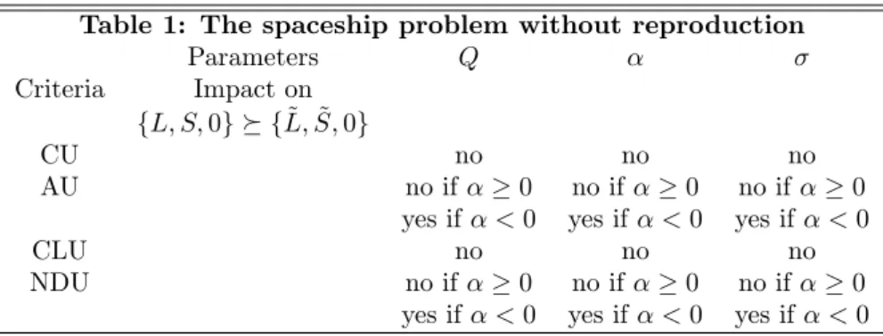
Let us now collect our results regarding the social ranking of lifetime-equal histories in a spaceship problem without reproduction. For that purpose, Table 1 shows the sensitivity - or, alternatively, the invariance - of the social ranking of lifetime-equal histories to the structural parameters of the economy, under the four population ethics criteria under study.
3 1This is the case because, when = 1, the denominator of the …rst factor of the RHS is
0, and the second factor is negative, so that the RHS equals 1. Hence cannot be smaller than the RHS, and thus the condition on is never satis…ed.
3 2To see here why a dilution of lifetime on more people may be socially desirable under
NDU, we can, here again, compute the welfare change from a rise in L compensated by a fall in S in such a way as to maintain the total lifetime constant, i.e. @W@Lc =@W@L +@W@S @S@L:
L 1 Q L " + (1 )S1 (1 )S (1 S1 )2 # L 1 (1 ) 1 S
The term in brackets is negative. Hence, given that the second term is also negative if > 0, we have that@W@Lc < 0under 0. But once < 0, the second term is positive, and adding new persons while reducing S may be welfare-increasing, as under AU.
Table 1: The spaceship problem without reproduction Parameters Q Criteria Impact on fL; S; 0g f ~L; ~S; 0g CU no no no AU no if 0 no if 0 no if 0
yes if < 0 yes if < 0 yes if < 0
CLU no no no
NDU no if 0 no if 0 no if 0
yes if < 0 yes if < 0 yes if < 0 Table 1 illustrates the major division between our four normative criteria: whereas rankings of lifetime-equal histories under CU and CLU are invariant to the total available space, as well as to individual preferences, the same is not true under AU and NDU once is negative. Therefore, the sign of the intercept of the temporal utility function is a major discriminant factor among our normative criteria. When 0, the social planner selects the lifetime-equal history with the lowest initial population and the largest survival rate, under all utilitarian criteria. However, if < 0, the solutions under AU and NDU become dependent on the total available space and the preference parameter . In sum, there are two distinct ways to interpret Table 1. On the one hand, one may start from what one regards as a morally relevant or a simply em-pirically observable piece of information, and select, on the basis of that, a normative criterion. On the other hand, one may, from the start, opt for one criterion, and then consider what a¤ects the solution under that particular view. If one has no obvious reason to believe in a particular population ethics criterion a priori, Table 1 will be interpreted in the former way, and one can then advocate in favour of CU or CLU on several distinct grounds. For instance, CU and CLU do not require any information on individual preferences to give a solution to the spaceship problem without reproduction. Given the di¢ culty to estimate empirically, the invariance of rankings to can be regarded as a strong argument in favour of CU and CLU. Alternatively, one may argue that the solution to the spaceship problem should be invariant to the spaceship size Q, and defend CU and CLU on those grounds.33
4
The spaceship problem (2): reproduction
Let us now turn to the more general problem where the population of the spaceship can reproduce itself. This amounts to relaxing the postulate of a zero fertility rate n (i.e. Assumption A11). That more general spaceship problem can be regarded as including the widely debated issue of the optimal population existing on the Earth. After all, the Earth can be regarded as a spaceship with living conditions allowing the reproduction of its population.
To study the spaceship problem with reproduction, we will, here again, ex-amine how a social planner ranks lifetime-equal histories fL; S; ng and f ~L; ~S; ~ng.
3 3The intuition supporting the property of invariance to Q is the following: once the total
time to be lived is …xed, why should the discovery of a new place to live (e.g. a new galaxy) question the past selection of the best history? Given the - so far un…nished - exploration of the Universe, one may want the current solution of the spaceship problem - i.e. given the currently known Q - to remain valid even if one discovers a new place in the future.
For the ease of presentation, we consider here the comparison of lifetime-equal histories with the same initial population sizes (i.e. L = ~L), that is, the number of pioneers is equal in all histories. Such a way to proceed is actually quite natural, as the population of the Earth (or any other spaceship) ‘is what it is’, so that a social planner governing a spaceship has no other choice than to take the initial population L as given. Indeed, from a policy perspective, the only possible interventions concern future fertility n or longevity 1=1 S, but one can hardly change the initial population size L. Thus assuming common initial populations L = ~L seems plausible.
Assumption A12 The initial population size L is equal in all histories. Under L = ~L, and assuming a …nite number of life-periods (i.e. Sn < 1), lifetime-equal histories fL; S; ng and f ~L; ~S; ~ng are such that
1
(1 S)(1 nS) =
1 (1 S)(1~ ~n ~S)
A history with longer lives will also exhibit, for a given total number of life-periods, a lower fertility: S S () n~ n. In the spaceship problem~ with reproduction, comparing two lifetime-equal histories fL; S; ng and fL; ~S; ~ng amounts to comparing two histories for which:
1 S~ 1 S =
1 nS 1 n ~~S
that is, there is an equality of the ratios of strength of mortality [i.e. 1 S] (LHS) and strengths of fertility [i.e. 1 nS1 ] (RHS) for histories fL; S; ng and fL; ~S; ~ng having an equal number of life-periods (i.e. for which P = ~P ). Intuitively, if one history exhibits a larger fertility (i.e. 1
1 ~n ~S > 1
1 nS) than another history
with the same total number of life-periods, it must also be characterized by a larger strength of mortality (i.e. 1 S > 1~ S).
4.1
The Classical Utilitarian solution
As in the problem without reproduction, it is tempting to believe, at …rst glance, that CU will exhibit a populationist bias, and lead to the selection of a large fertility rate and a low survival rate. However, Proposition 5 suggests that this is not necessarily the case.
Proposition 5 Assume A1-A10 and A12. Consider two lifetime-equal histo-ries fL; S; ng and fL; ~S; ~ng, with S < ~S and n > ~n. The CU planner prefers fL; S; ng to fL; ~S; ~ng if and only if:
1 X t=0 St1 n t+1 1 n 1 X1 t=0 ~ St1 n~ t+1 1 n~ 1
Proof. See the Appendix.
As in the problem without reproduction, the rankings under CU are indepen-dent from the size of the spaceship Q. Moreover, the social ordering of lifetime-equal histories is also independent from the intercept . Furthermore, the initial
size of the population, L, has no e¤ect on the social ordering over lifetime-equal histories. Thus whatever the initial population is, CU ranks lifetime-equal histo-ries in the same manner. For those who appreciate the independence of rankings from the past, that property of CU is highly valuable.
However, note that, despite some common aspects with the spaceship prob-lem without reproduction (e.g. independence of the solution from Q and ), there exists, nonetheless, a fundamental di¤erence between Propositions 1 and 5. Whereas CU leads, in the absence of reproduction, to the selection of the history with the lowest L and the highest S, it is di¢ cult here to see whether CU recommends a population with a high survival and a low fertility or the op-posite. Di¤erent combinations of n and S yield di¤erent intertemporal paths of qt, and the ranking of lifetime-equal histories depends on how sensitive temporal
welfare is to the space available for each person (i.e. the parameter ).
Thus, the introduction of reproduction on the spaceship alters the conclu-sions drawn in the no reproduction case. Under 0 < < 1, it is now hard to see whether a CU planner would opt for a pre-demographic transition state (i.e. with a high n and a low S), or, alternatively, for a post-demographic tran-sition state (i.e. with a low n and a high S), as long as the total number of life-periods is the same, whereas, in the problem without reproduction, the CU solution always consisted in choosing the highest survival rate.
Finally, note that it is nonetheless possible to see what the CU social ranking in the extreme cases where = 0 and = 1.34
Corollary C3 Under = 0, the CU planner is indi¤erent between any lifetime-equal histories.
Corollary C4 Under = 1, the CU planner is indi¤erent between any lifetime-equal histories.
4.2
Average Utilitarianism
AU yields an ambiguous ranking in the absence of reproduction, depending on the intercept of the temporal utility function . Once reproduction is allowed, things do not become more clear, as stated in Proposition 6.
Proposition 6 Assume A1 to A10 and A12. Consider two lifetime-equal his-tories fL; S; ng and fL; ~S; ~ng, with S < ~S and n > ~n. The AU planner prefers fL; S; ng to fL; ~S; ~ng if and only if:
1 X t=0 St1 n t+1 1 n 1 1 S 1 S~ 1 X t=0 ~ St1 n~ t+1 1 n~ 1 Q L 1 Sn 1 1 S~ 1 1 S or, in terms of , Q L (1 Sn)(1 S)(1~ S) ~ S S "1 X t=0 St1 n t+1 1 n 1 1 S 1 S~ 1 X t=0 ~ St1 n~ t+1 1 ~n 1 #
Proof. See the Appendix.
Contrary to Proposition 5, three factors a¤ect the social ranking of lifetime-equal histories. First, the intercept of the temporal utility function ; second,
the total space available Q; third, the initial population size L. All this makes the AU solution likely to di¤er from the CU solution. Let us brie‡y examine the impact of those three determinants of the social ordering.
The impact of depends on its sign. Clearly, whatever is positive or negative, the LHS of the …rst condition in Proposition 6 is smaller than the LHS in Proposition 5. Hence, if 0, AU recommends a lifetime-equal history with a higher S and a lower n in comparison with the one under CU. However, under < 0, the RHS of the …rst condition in Proposition 6 becomes negative, so that it is no longer certain that AU selects a lifetime-equal history with a higher S and a lower n than CU. We may actually observe the opposite, because of the dilution e¤ect mentioned in the problem without reproduction.
Regarding the impact of the available space Q, it is easy to see that the smaller Q is, the larger the RHS of the …rst condition in Proposition 6 is, so that lifetime-equal histories with a high S and a low n are more likely to be selected (under 0). The opposite prevails under su¢ ciently negative, on the grounds of the dilution e¤ect (see above).
As far as the in‡uence of the initial population L is concerned, Proposition 6 suggests that the larger L is, the larger the RHS of the …rst condition for fL; S; ng fL; ~S; ~ng is, so that AU is more likely to select a lifetime-equal history with a high S and a low n, under 0. However, under < 0, a larger L may make the dilution of misery necessary, leading to a lifetime-equal history with a high n and a low S. The AU solution is thus, unlike the CU solution, dependent on the initial population size, and, thus, dependent on the past.
Finally, it should be noticed that the AU solution di¤ers here from what it is in the absence of reproduction. True, as without reproduction, AU does not necessarily lead to the selection of the lifetime-equal history with the low-est population size and the larglow-est life expectancy when temporal welfare is negative. But, more importantly, even for a non-negative is the selection of lifetime-equal histories with the highest S no longer certain here, contrary to what prevailed in the absence of reproduction.
4.3
Critical-Level Utilitarianism
The preferences of a CLU social planner over lifetime-equal histories fL; S; ng and fL; ~S; ~ng are characterized by Proposition 7.
Proposition 7 Assume A1 to A10 and A12. Consider two lifetime-equal his-tories fL; S; ng and fL; ~S; ~ng, with S < ~S and n > ~n. The CLU planner prefers fL; S; ng to fL; ~S; ~ng if and only if:
1 X t=0 St1 n t+1 1 n 1 X1 t=0 ~ St1 n~ t+1 1 n~ 1 Q L u^ 1 1 nS 1 1 n ~~S Proof. See the Appendix.
Note that, under ^u = 0, the condition stated in Proposition 7 collapses to the condition under CU (Proposition 5). Note also that, under ^u equal to average lifetime welfare, the condition for fL; S; ng fL; ~S; ~ng coincides with the condition under AU (Proposition 6). Therefore, we can interpret CLU as a natural generalization of CU and AU.
Having stressed this, it remains that the CLU solution to the spaceship problem remains somewhat closer, in some sense, of the CU one in comparison to
the AU one. The reason why this is so is that the condition stated in Proposition 7 does not depend on , exactly like the condition under CU. That result is somewhat surprising, as one would expect the ranking under CLU to depend on how large the critical level ^u is with respect to the intercept . But here again, and exactly as in the case of CU, the level of the intercept of the temporal utility function does not matter.
However, the proximity of the CLU and CU solutions has some limits. Firstly, the size of the initial population L in‡uences the solution of the space-ship problem here, unlike under CU. The larger L is, the more likely the pref-erence for a lifetime-equal history with a lower fertility and a lower mortality is. Thus, the extent to which the demographic transition is valuable depends, under a …xed available space, on the size of the population that undergoes the transition. The larger the population is, the more bene…cial the demographic transition is. Secondly, note that the solution to the spaceship problem with reproduction depends, under CLU, on the spaceship size Q, unlike what it was the case under CU. This constitutes another important distinction between the two normative criteria in the present context.
4.4
Number-Dampened Utilitarianism
Let us now consider the rankings induced by NDU over lifetime-equal histories. Proposition 8 Assume A1 to A10 and A12. Consider two lifetime-equal his-tories fL; S; ng and fL; ~S; ~ng, with ~S > S and n > ~n. The NDU planner prefers fL; S; ng to fL; ~S; ~ng if and only if:
1 X t=0 St1 n t+1 1 n 1 1 S 1 S~ 1 X1 t=0 ~ St1 n~ t+1 1 n~ 1 (Q) L (1 Sn)1 1 1 S ~~n 1 1 S~ 1 1 Sn 1 1 S or, in terms of , Q L (1 Sn)1 P1t=0 St 1 n1 nt+1 1 1 S 1 S~ 1 P 1 t=0 S~t 1 n~ t+1 1 n~ 1 1 1 S ~~n 1 1 S~ 1 1 Sn 1 1 S
Proof. See the Appendix.
If equals 1, the condition for fL; S; ng nL; ~S; ~no coincides with the one under CU (Proposition 5), while, under equal to 0, we are back to the AU condition (Proposition 6). Thus, exactly as in the absence of reproduction, NDU is, like CLU, a generalization of standard utilitarian criteria.
However, a signi…cant di¤erence remains between the two criteria: the or-dering under CLU over lifetime-equal histories is invariant to the intercept of the temporal utility function , contrary to the ordering under NDU, which depends on whether is positive or negative, large or small. That result does not surprise us, as this was already present in the simpler version of the space-ship problem considered in Section 3. But the present analysis reveals that this fundamental di¤erence between CLU and NDU is robust to the introduction of reproduction on the spaceship.
4.5
A synthesis
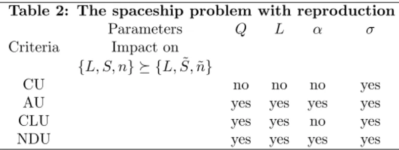
To sum up, Table 2 shows the determinants of the social ranking of lifetime-equal histories in the spaceship problem with reproduction.
Table 2: The spaceship problem with reproduction
Parameters Q L
Criteria Impact on fL; S; ng fL; ~S; ~ng
CU no no no yes
AU yes yes yes yes
CLU yes yes no yes
NDU yes yes yes yes
Table 2 illustrates that our four normative criteria are not sensitive to the same information. The CU solution is the only one that is invariant to the spaceship size Q and to the initial population L. Hence, for decision-makers who would like their decisions to be independent from the past, CU seems to be the adequate criterion. The three other criteria depend all on how large the initial population is, and on how large the spaceship is. But those three remaining criteria di¤er from each others, as the AU and the NDU solutions depend on the intercept of the temporal utility function , contrary to the CLU solution. Therefore if one considers that cannot be observed, and, thus, cannot serve as a basis for the social planner’s ranking, it follows that, if Q and L are regarded as relevant, only the CLU solution is adequate. Finally, note that the AU and NDU solutions are both dependent on the four factors explicitly listed in Table 2. Thus those two normative criteria are equally demanding in terms of information, and di¤er only in how that information is treated.
The comparison of Table 2 (spaceship with reproduction) with Table 1 (spaceship without reproduction) shows that the parameter , which captures the sensitivity of temporal welfare to space per head, plays now a crucial role whatever the criterion is, unlike what was the case in the absence of reproduc-tion, where was benign (except under a negative under AU and NDU).
The role of other parameters is also strengthened once reproduction is in-troduced. The total space available Q was, in general, benign in the absence of reproduction (except under a negative under AU and NDU), but once repro-duction is allowed, Q becomes a major variable for all normative criteria except CU. Moreover, the intercept plays now a signi…cant role than in the spaceship problem without reproduction.
5
The spaceship problem (3): stationary
space-ship
While we focused so far on a spaceship whose population would only enjoy, as a whole, a …nite total number of life-periods, that restriction may appear quite pessimistic, as this implies a population that will vanish asymptotically towards 0 (even though it may exhibit some growth during a part of history). That …niteness assumption, although analytically convenient, presupposed the impossibility for Mankind to have an in…nite history, because of some constraints
preventing the perpetual survival of life in the spaceship. In the case of human-made spaceships like rockets, this constraint would follow, for instance, from a limit in the quantity of oxygen available. But in the case of more complex spaceships with ecosystems (like the Earth), this restriction seems less plausible. If one believes in human capacity to overcome technical di¢ culties, the …nite-ness assumption Sn < 1 must be relaxed. This is the reason why we will here depart from A10, and consider instead the case of a stationary spaceship, that is, a spaceship with a …nite constant asymptotic population. Actually, it is not di¢ cult to see that the constancy of the asymptotic population requires, in this framework, nothing else than nS = 1. Indeed, the constancy of the population at a given point in time requires an equality of births and deaths
L(Stnt) = L(S tnt) Sn (1 S) + L(Stnt) S2n2 S(1 S) + ::: + LS t 1(1 S) = L(S tnt) Sn (1 S) 1 + 1 n+ 1 n2 + ::: + 1 nt 1
Hence a constant asymptotic population (i.e. t ! 1) requires 1 = 1 S
Sn S
If Sn S1 S > 1, the population tends to zero asymptotically, as the long-run number of deaths exceeds the long-run number of births. On the contrary, if
1 S
Sn S < 1, the population tends to in…nity, as the long-run number of births
exceeds the long-run number of deaths. Finally, it is only under Sn S1 S = 1, that is, under Sn = 1, that the population is asymptotically constant. This is the assumption we will make in this section.
Assumption A13The population of the spaceship converges asymptot-ically towards a positive constant, i.e. Sn = 1.
Note that, under that assumption, the long-run level of the population of the spaceship will be exactly equal to the total number of life-periods under no reproduction on the spaceship. That equivalence result is stated below. Proposition 9 Under an initial population L, a survival rate S and a fertility rate n such that nS = 1, the long-run population size equals the total number of life-periods in the absence of reproduction, i.e. L
1 S.
Proof. See the Appendix.
The intuition behind that equivalence result is the following. Both numbers - the total number of life-periods under n = 0 and the total population size - have, at time 0, the same level, equal to L. The number of periods under n = 0 becomes, at time 1, equal to L + LS, while the number of persons under nS = 1 becomes, at time 1, equal to SL + SLn, which is SL + L. At t = 2, the total number of periods in the spaceship without reproduction is L + SL + S2L,
while the number of persons under nS = 1 is S2L + S2Ln + S2Ln2, that is,
S2L + SL + L, and so forth. We are thus in presence of two sums whose terms
are the same, yielding Proposition 9.
Having stressed that equivalence result, there remains a fundamental dif-ference between a spaceship without reproduction and a stationary spaceship:
while the former involves a …nite number of life-periods, the latter involves an in…nite number of life-periods. Formally, the total number of life-periods is
P = L
(1 S)(1 Sn)
so that, under Sn = 1, the number of life-periods is in…nite. Hence any two histories fL; S; ng and f ~L; ~S; ~ng with Sn = ~S ~n = 1 have an in…nite P .
The non-…niteness of total lifetimes is really problematic for an aggregative doctrine like utilitarianism, whatever the precise form it takes, because such an aggregative doctrine aims at taking into account the utilities at all life-periods, so that the in…nity of life-periods makes the utilitarian planner deal with quantities that are no longer …nite. There exist two broad families of solutions to that problem. On the one hand, one can depart from utilitarianism, and turn towards a less aggregative ethical standard (e.g. adopting a Maximin objective focusing on the worse-o¤ cohort). On the other hand, one may keep the utilitarian doctrine, but restrict the informational basis that is taken into account.
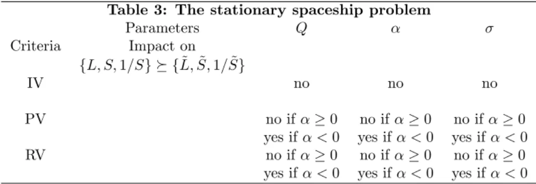
In the rest of this section, we will take the second road, and remain within utilitarianism. What we shall do is to reduce social welfare comparisons to what prevails at the stationary state, that is, at the population level that, once reached, will prevail forever in the spaceship. In other words, we will concentrate on the living conditions faced by all generations succeeding to each others once the steady-state is reached, each generation enjoying a …nite life, and giving birth to another generation that will also enjoy exactly the same living conditions (i.e. same space per head). That focus on the stationary state is a way to ‘extract’the spaceship from time, that is, from history. This means that all things occurring outside the steady-state will not be taken into account here.35
Therefore, in order to characterize the solutions of the stationary spaceship problem, we will, in this section, focus on histories that are not only lifetime-equal, which is the case of all histories under Sn = 1, but on histories that are population-equal, in the sense that these yield the same long-run population.
De…nition D7Two histories fL; S; ng and f ~L; ~S; ~ng are population-equal if these yield the same asymptotic population size, that is, if and only if
L 1 S =
~ L 1 S~
Note that, given Sn = 1, the comparison of population-equal histories amounts to focusing on two demographic parameters: the size of the pioneer group, L, and the survival proportion S. Here again, this leads us back, in some way, to the spaceship problem without reproduction: comparing two population-equal histories fL; S; ng and f ~L; ~S; ~ng amounts to comparing his-tories fL; S; 1=Sg and f ~L; ~S; 1= ~Sg with 1 SL = L~
1 S~, exactly as the spaceship
problem without reproduction amounts to comparing histories fL; S; 0g and f ~L; ~S; 0g with 1 SL = L~
1 S~:
3 5Naturally, such a reduction, which is allowed by the existence of a state of constant
population, is far from neutral on ethical grounds: ignoring a whole span of history and concentrating on a ‘timeless’ spaceship is obviously a simpli…cation. However, given that the stationary state will be faced by an in…nite number of people, the reduction of history to the timeless stationary spaceship seems legitimate, as a …rst approximation.