HAL Id: cea-02614140
https://hal-cea.archives-ouvertes.fr/cea-02614140
Submitted on 20 May 2020HAL is a multi-disciplinary open access archive for the deposit and dissemination of sci-entific research documents, whether they are pub-lished or not. The documents may come from teaching and research institutions in France or abroad, or from public or private research centers.
L’archive ouverte pluridisciplinaire HAL, est destinée au dépôt et à la diffusion de documents scientifiques de niveau recherche, publiés ou non, émanant des établissements d’enseignement et de recherche français ou étrangers, des laboratoires publics ou privés.
J.-M. Gatt, R. Henry, I. Zacharie-Aubrun, C. Langlois, S. Meille
To cite this version:
J.-M. Gatt, R. Henry, I. Zacharie-Aubrun, C. Langlois, S. Meille. Identification of fracture param-eters for irradiated nuclear fuel. SMIRT25 - 25th Conference on Structural Mechanics in Reactor Technology, Aug 2019, Charlotte, United States. �cea-02614140�
Transactions, SMiRT-25 Charlotte, NC, USA, August 4-9, 2019
Division II
Identification of fracture parameters for irradiated nuclear fuel
Jean-Marie Gatt1, Ronan. Henry2, Isabelle. Zacharie-Aubrun1, Cyril Langlois3, Sylvain Meille3
1
Engineer, CEA, DEN, DEC, F-13108 Saint-Paul-Lez Durance, France (jean-marie.gatt@cea.fr)
2 PHD, Université Lyon,INSA Lyon MATEIS UMR CNRS 5510, Villeurbanne, France 3
Professor, Université Lyon,INSA Lyon MATEIS UMR CNRS 5510, Villeurbanne, France
INTRODUCTION
This paper deals with the fracture characteristics of UO2 fuel. At low temperature (<900 °C) this ceramic
has a brittle behavior in traction. The knowledge of fracture parameters for irradiated UO2 fuel is useful to
model and understand the behavior of the fuel in reactor. The crack model used in numerical simulations of the fuel rod behavior is based on two main parameters: the critical stress and the fracture toughness. The aim of this article is to analyze fracture tests to identify these two parameters at different scales. To obtain the rupture parameters, we use two kinds of sample (smooth and notched samples) with three sizes: large (28x4x4 mm3), small (10x1.5x1.5 mm3) and micrometric (13x4x3 µm3). Fracture toughness is a local
parameter that can be measured using notched samples, so it depends weakly on the sample size. Nevertheless, critical stress seems to depend on the size of the sample. In this article, this problem is discussed using analytical and numerical approaches.
FRACTURE MODELS
To model the cracks initiation and propagation we used a simple cohesive zone model (Dugdale 1960 and Barenblatt 1962). The model can be described by the following equations, with corresponding parameters as defined in Figure 1.
1
2 (1)
Figure 1: Stress versus displacement (crack opening) of the cohesive zone model To verify the model consistency ( , we have to add the following condition:
2 (2) The parameter must be sufficiently high to avoid an important displacement before reaching critical stress , but not too large to avoid numerical instabilities. In the certain range of values, the response of the model is independent of this parameter. In our previous studies (Gatt 2015) we found: 6. 10 / .
In that case, this model depends only of two “physical” parameters, the critical stress and fracture toughness . From equation (1), the following behavior law can be deduced:
! " # #
0
(3)
This model can be modified to be used directly in finite elements approach (Michel 2008). In this case, the cohesive law described in Figure 2 is determined by two parameters: the critical stress and $%&& '()
*(+ , the cracking softening modulus (+ being the finite element length (the half distance between the
Gauss points) in the direction perpendicular to the crack plane).
Figure 2: Smeared crack model
ANALYTICAL APPROACH
As shown in Gatt 2015, the goal is to evaluate the critical stress from the study of smooth specimens submitted to a three points bending test (see Figure 3for notations). In that objective, we are going to use an approach introduced by Leguillon 2002, based on two parameters: the critical stress and the fracture toughness or the critical stress intensity factor ( , $ in plane stress ($ is the Young’s modulus). To observe a fracture, we need to verify these two criteria:
-5/0 √7./0 1234
123 4 8 9: 123 ;+
< = (4)
./0 and 5/0 (with 0 7/9 : see Figure 3) are two following functions defined in (5) and (6):
./0 1 20 >7 5/0 /1 ? 20 /1 0√0 /0 @/ (5)
25 Conference on Structural Mechanics in Reactor Technology Charlotte, NC, USA, August 4-9, 2019 Division II
/0 1.99 0/1 0 /2.15 3.930 ? 2.70 (6)
This approach is consistent with the cohesive zone model and smeared crack model. For macroscopic samples (28x4x4 mm3 and 10x1.5x1.5 mm3), when the critical stress is reached, the damage of the sample begins (the stress decreases). The sample breaks when in the same time, on a length 7E the two criteria are verified. We observe that 7E stays small compared to sample thickness (0F is small), so the first equation of (5) is a good approximation of the stress distribution.
Figure 3: Three points bending sample
The failure of smooth specimen is obtained if the two following conditions are verified: G./0F5/0F √9H
H
(7)
According to the first equation of system (4) and the definition of ./0F in (7), we have:
H 1 20F
(8)
And from the second equation of system (4) we have: 5/0F
√9 H
(9)
These two last equations (8) and (9) allow plotting the curves shown in Figure 4 and Figure 5.
Figure 4: A function Figure 5: Critical stress evaluation from fracture stress
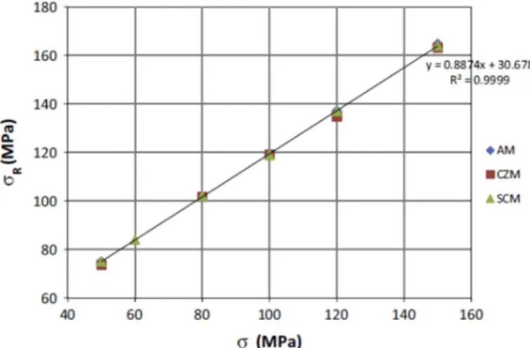
If we compare analytical approach and numerical approach, we obtain a good correspondence as shown in Figure 6.
Figure 6: Comparison of the three approaches: Cohesive Zone Model, Smeared Crack Model and Analytical Model (respectively CZM, SCM and AM).
TESTS RESULTS
Tests on macroscopic (28x4x4 mm3 and 10x1.5x1.5 mm3) (Gatt 2015) and microscopic (15x4x4 µm3)
(Henry 2019) notched and smooth UO2 samples have been performed. Macroscopic samples
For macroscopic samples (Gatt 2015), the rupture stress is evaluated between 104 and 141 MPa for small samples and between 126 MPa and 144 MPa for large samples. The critical stress intensity factor is evaluated at 2 MPa.m0.5(±0.5).
Numerical simulations shown that the critical stress can be taken equal to 100 MPa.
Microscopic samples
In this case, the shape and the loading of samples are different for manufacturing reasons. Whereas macroscopic samples are submitted to three points bending tests (Figure 3) with an imposed displacement rate, microscopic samples are submitted to simple bending tests with an imposed force rate. The microscopic samples have been milled in the fuel with a focused ion beam (FIB) of an Aurega FIB SEM (Scanning Electron Microscope) of Carl Zeiss (Figure 7). The cantilevers were bent in the FIB SEM with a CSM NHT2 nano-indenter at a constant speed of 0.05 mN/s until the fracture. Each micro-cantilever was machined into a single grain of an anisotropic crystalline sample of UO2 (Henry 2019).
25 Conference on Structural Mechanics in Reactor Technology Charlotte, NC, USA, August 4-9, 2019 Division II
The critical stress intensity factor has been evaluated on notched microscopic sample at 1.96 MPa m0.5(±0.3). This evaluation is consistent with the macroscopic testing. At microscopic scale, the size of the sample being smaller than the grain size, tests in different crystalline plane orientations have been performed. These tests show a small evolution (±5%) of the critical stress intensity factor with the crystalline plan targeted.
Tests on smooth microscopic samples have also been performed. For a sample size of L=15.67 µm, W = 3.03µm, C = 1.34 µm and B = 3.77 µm (see notations Figure 8) fracture stress was evaluated at 3.06 GPa, using the analytical equations (10), (11) and (12).
INTERPRETATION OF THE TESTS RESULTS ON MICROSCOPIC SAMPLES
To assess the critical stress from microscopic tests, the same approach is used: analytical and numerical approaches.
Analytical analysis
For analytical approach, we assume a perfect embedding of the sample. In this case, the maximal stress is (see Figure 8 for notations):
123 123<. +. = *
(10)
With 123the maximal load and <* the inertia defined in equation (12). The position z of the gravity center is:
= 3. I ? J² ? 3. J. I6. I ? 3. J (11)
In addition, the inertia moment reads: <* L. I @ 12 ? L. I != I2 " ?L. J @ 36 ?L2 . J M/8 = ? !J3"N (12)
Figure 8: Notations for microscopic sample (pentagonal section)
For pentagonal sample, the function A(x) calculated by finite element analysis by Chan 2016 (with:0 O
P)
is :
In the case of pentagonal cantilever, Figure 4 and Figure 5 are transformed into following Figures:
Figure 9: A function Figure 10: Critical stress evaluation from fracture stress
If we perform the same analysis as for macroscopic samples, the critical stress obtained is much higher than for macroscopic samples: 2.8 GPa. This result implies that the critical stress depends of the size of the sample.
Numerical analysis: Elastic evaluation
To solve this problem, we have tried, in a first time, to evaluate more accurately the fracture stress through numerical simulation, assuming a perfect embedding. The fracture stress is nearly equal to analytical one as shown in Figure 11. In Figure 11 we also observe an important stress concentration due to embedding (for which z equals zero).
Figure 11: Stress evolution along the length of the sample
In a second time, we have considered a more realistic embedding (Figure 13), according to Figure 7, the numerical maximal stress is lower but stays very high (see Figure 12).
25 Conference on Structural Mechanics in Reactor Technology Charlotte, NC, USA, August 4-9, 2019 Division II
Figure 12: Stress evolution along the length of the sample
Numerical simulation with smeared crack model
The calculations have been performed using the meshing by finite elements presented in Figure 13.
Figure 13 Meshing of the structure
We took a critical stress equal to 100 MPa, and we impose a force at point C (Figure 13) as in the tests. If we plot the stress evolution along the thickness of the beam (between points A and B in Figure 13), we can observe, in Figure 15, an increase of the stress at different normalized times (at time 0 F=0 and at time 1 F=Fmax=1.77.10-3 N). At t=0.04, the critical stress is reached at point A. At t=0.08 the critical stress is
reached on a larger thickness. Then, we observe a propagation on the damage zone. Nevertheless, we don’t observe a decrease on the stress in this area. This means that the available energy is not sufficient to generate damage. In the compression part, the stress increases to maintain the balance of the flexion moment.
A B
Figure 14 Stress evolution along the thickness of the beam
If we continue to load, an evolution of the damage area is observed in the Figure 15. Nevertheless, we don’t observe a decrease ( ) of the stress showing an evolution of the damage.
Figure 15 Stress evolution along the thickness of the beam
If we plot the evolution of the stress along the length of the sample (between points A and C in Figure 13), we observe (Figure 16) an increase of the stress up to the critical stress (t<0.04). The propagation of the damage is observed on the length and a local decrease of the stress from time t = 0.15. At t=0.41 the sample is broken (the stress reaches zero).
We observe that the fracture doesn’t appear at the embedding but in a close area, as noted in the experimental observations. In this case, the maximal stress can be evaluated around 1.25 GPa. This value is important but smaller than the experimental value (3.06 GPa). Nevertheless, the stress is equal at 100 MPa between points A and C on all the length of the sample. This prediction does not seem to be physical.
25 Conference on Structural Mechanics in Reactor Technology Charlotte, NC, USA, August 4-9, 2019 Division II
Figure 16 Stress evolution along the length of the beam
If we take the theoretical value for critical stress (that is to say 2.8 GPa), and if we impose a displacement to evaluate more accurately the moment of the rupture (see Figure 17), then the stress failure calculated is 3.03 GPa. This value is closed to the experimental value 3.06 GPa.
Figure 17: Stress and force versus displacement
CONCLUSION
To model the fracture of UO2 samples in bending, we used a smeared crack model based on a zone cohesive
model. This model allows a good interpretation of tests in three points bending on macroscopic samples. In the framework of this first analysis, the parameters of the model (fracture toughness and critical stress) have been identified. To extrapolate this identification at the microscopic scale, some difficulties appear to interpret the critical stress. If we take the same critical stress (100 MPa) for all the scales, the simulation shows a rupture at 1.2 GPa for microscopic scale. If we take the theoretical critical stress at 2.8 GPa, we obtain the same failure stress as measured during the experimental tests. This study shows that the critical stress is not a local property but depends of the statistic of the defaults inside the material. There are much more defaults in a macroscopic sample than in a microscopic. Therefore, the critical stress is higher in this last one.
REFERENCES
Dugdale, D., S. (1960), Yielding of steel sheets containing slits, journal of Mechanics and physics of Solids, 8, 100-104
Barenblatt, G., I. (1962), The mathematical theory of equilibrium cracks in brittle fracture, Advance in Applied Mechanics 7, 55-129
Gatt, J-M, Sercombe, J., Aubrun, I., Menard, J-C, (2015), Experimental and numerical study of fracture
mechanisms in UO2 nuclear fuel, Eng. Fail. Anal. 47, 299-311
Michel, B., Sercombe, J., Thouvenin, D., Chatelet, R. (2008). 3D Fuel cracking modelling in pellet cladding
mechanical interaction. Eng. Fract. Mech 75, 3581-3598.
Leguillon, D. (2002). Strength or toughness: a criterion for crack onset at a notch, Eur J Mech A Solid 21 61-72.
Henry, R., (2019), Caractérisation à l’échelle locale et à température ambiante des propriétés mécaniques
du combustible irradié, PhD, University of Lyon, INSA-Lyon.
Anderson; T., L. (1991), Fracture mechanics. Fundamentals and applications. Library of congress. ISBN 0-8493-4277-5.
Chan, H., Robert, S., G., Gong, J., (2016), Micro-scale fracture experiments on zirconium hybrids and
phase boundaries, J. Nucl. Mater., Vol 475, 105-112
H. Chan, S. G. Roberts, and J. Gong, Micro-scale fracture experiments on zirconium hydrides and phase
boundaries, J. Nucl. Mater., vol. 475, pp. 105–112, 2016.
Acknowledgements: The autors thank EDF and FRAMATOME for their technical and finacial support to