HAL Id: halshs-00586878
https://halshs.archives-ouvertes.fr/halshs-00586878
Preprint submitted on 18 Apr 2011HAL is a multi-disciplinary open access archive for the deposit and dissemination of sci-entific research documents, whether they are pub-lished or not. The documents may come from teaching and research institutions in France or abroad, or from public or private research centers.
L’archive ouverte pluridisciplinaire HAL, est destinée au dépôt et à la diffusion de documents scientifiques de niveau recherche, publiés ou non, émanant des établissements d’enseignement et de recherche français ou étrangers, des laboratoires publics ou privés.
New economic geography: A guide to transport analysis
Miren Lafourcade, Jacques-François Thisse
To cite this version:
Miren Lafourcade, Jacques-François Thisse. New economic geography: A guide to transport analysis. 2008. �halshs-00586878�
WORKING PAPER N° 2008 - 02
New economic geography:
A guide to transport analysis
Miren Lafourcade
Jacques-François Thisse
JEL Codes: L91, R12, R58
Keywords: economic geography, transport costs, regional
disparities
P
ARIS-
JOURDANS
CIENCESE
CONOMIQUESL
ABORATOIRE D’E
CONOMIEA
PPLIQUÉE-
INRA48,BD JOURDAN –E.N.S.–75014PARIS TÉL. :33(0)143136300 – FAX :33(0)143136310
www.pse.ens.fr
New Economic Geography:
A Guide to Transport Analysis
*Miren Lafourcade
Université de Valenciennes and Paris School of Economics Jacques-François Thisse
CORE, Université catholique de Louvain and Ecole Nationale des Ponts et Chaussées 12 February 2008
Contents
1. Introduction... 2
2. The rise of spatial inequalities in pre-World War I Europe ... 5
3. Do lower transport costs foster more spatial inequality?... 6
3.1 The basic framework ... 7
3.2 The mobility of capital... 8
3.3 The mobility of labor... 9
3.4 A welfare analysis of the core-periphery model ... 12
3.5 A growth approach to regional disparities... 14
4. The bell-shaped curve of spatial development ... 15
4.1 Imperfect labor mobility... 15
4.2 The role of non-tradable goods ... 17
4.3 Vertical linkages... 18
4.4 The spatial fragmentation of firms... 19
5. How to measure transport costs and their impact on the distribution of activities?... 21
5.1 The measurement of transport costs... 21
5.2 How transport costs affect the location of activities: the simulation of large-scale models ... 25
6. What are the policy implications and where should we go now?... 27
References... 31
Abstract
The paper surveys the main contributions of new economic geography from the point of view of transport analysis. It shows that decreasing transport costs is likely to exacerbate regional disparities. However, very low transport costs should foster a more balanced distribution for economic activities across space. Thus, the spatial curve of development, which relates the degree of spatial concentration to the level of transport costs, would be bell-shaped. The paper also provides a detailed discussion of the main determinants of transport costs, which remain fairly large in most countries. It concludes with a discussion of some policy implications.
Key-words: economic geography, transport costs, regional disparities JEL classification: L91, R12, R58
*
This paper has been prepared for the Handbook in Transport Economics, edited by André de Palma, Robin Lindsey, Emile Quinet and Roger Vickerman. We gratefully acknowledge André de Palma and Robin Lindsey for insightful comments.
1. Introduction
Just as matter in the solar system is concentrated in a small number of bodies (the planets and their satellites), economic life is concentrated in a fairly limited number of human settlements (cities and clusters). The main purpose of economic geography is to explain why human activity is unevenly distributed across places and formed a large variety of economic agglomerations. Although using “agglomeration” as a generic term is convenient at a certain level of abstraction, it must be kept in mind that this concept refers to very distinct real world situations. At one extreme of the spectrum lies the North-South divide. At the other, restaurants, movie theaters, or shops selling similar products are often clustered within the same neighborhood, not to say on the same street.
In the foregoing examples, what drives the location of firms and consumers is the
accessibility to spatially dispersed markets, a fact that has been recognized for long both in spatial economics and regional science (Fujita and Thisse, 2002). Accessibility is itself measured by all the costs generated by the various types of spatial frictions that economic agents face in the exchange process. In the case of goods and services, such costs are called trade costs. Spulber (2007) refers to them as “the four Ts”: (i)Transaction costs that result from doing business at a distance due to differences in customs, business practices, as well as political and legal climates; (ii)Tariff and non-tariff costs such as different anti-pollution standards, anti-dumping practices, and the massive regulations that still restrict trade and investment; (iii)Transport costs per se because goods have to reach their consumption place, while many services remain non-tradable; and (iv)Time costs as, despite Internet and video-conferences, there are still communication impediments across dispersed distribution and manufacturing facilities that slow down reactions to changes in market conditions, while the time needed to ship certain types of goods has a high value. Because they stand for the costs of coordinating and connecting transactions between supplier and customer locations, trade costs are likely to stay on the center stage as they are crucial to the global firm. For example, trade and marketing costs accounts for 70% of the retail price of a Barbie doll (Spulber, 2007). Regarding the purpose of this chapter, it should be clear that trade costs, being the inherent attribute of exchanges across locations, are also central to the development of economic geography and its various applications.1
All distance-related costs having dramatically decreased with technological advances in transportation and the development of the new communication technologies (see, e.g. Bairoch, 1997), the following question suggests itself: what is the impact of falling transport and communication costs on he location of economic activity? Not surprisingly, but often forgotten, the answer depends on the spatial scale of analysis (Anas et al., 1998). New economic geography (henceforth NEG) is designed to operate
t
1
Trade costs involve both additive and multiplicative terms with respect to the mill price of goods, as excise and ad valorem taxes. Behrens (2006) has shown that both specifications lead to similar results regarding the spatial distribution of the industry.
at the regional level, thus implying that the focus is on interregional relationships.2 Furthermore, once it is recognized that trading goods is costly, it must equally be acknowledged that spatial frictions matter to firms and workers. Accordingly, NEG deals with situa ions in which the lack of mobility of goods and factors has equal relevance.
t
t t
t
Another fundamental ingredient of the space-economy is that production must display
increasing returns to scale, meaning that a proportional increase of all inputs yields a more than proportional increase of output. Otherwise, it would always be preferable to subdivide firms up to the point where all consumption places would accommodate very small units producing only for the local customers. Firms and households would thus reduce trade and their transport expenditures to zero, a situation that may be referred to as backyard capitalism. However, once economic activities are not perfectly divisible, the transport of goods or people between some places becomes unavoidable because production arises only in a few places.
It has been recognized for long that the trade-off between increasing returns in production and transport cos s is central o the understanding of the geography of economic activities (Koopmans, 1957; Krugman, 1995). As transport costs increase with distance, each plant supplies consumers located within a certain radius whose length depends on the relative level of freight costs and the intensity of increasing returns, whereas those located beyond this radius are supplied by other units. By modifying both transport costs and firms' technologies, the Industrial Revolution has deeply affected the terms of the above-mentioned trade-off in a way that is not easy to predict.
Even though it is true that economic activities are, at least to some extent, spatially concentrated because of natural features (think of rivers and harbors), it is reasonable to believe that these features explain only a fraction of the magnitude of regional disparities. This is why NEG has chosen to focus on pure economic mechanisms relying on the trade-off between increasing returns and different types of mobility costs. To achieve its goal, NEG borrows at will concepts and tools from microeconomics, trade theories and industrial organization. Although, as always in economics, everything depends on everything, geographical economics adds a new element to this: in all places, what is nearby has more influence than what is far away. Such a postulate concurs with the gravity prediction, that is, the intensity of flows of people, goods and ideas between two places is positively affected by their respective size and negatively by the distance separating them.
And indeed, in a world in which the tyranny of distance would be disappearing, empirical applications of gravity models run against this idea by showing that distance and borders remain major impediments to rade and interactions between spatially 2
This choice of a macroscopic scale allows us to avoid looking closely at the goings-on inside agglomerations. Indeed, the very nature of local interactions implies that most of them can be overlooked on the interregional scale.
separated firms and consumers (Head and Mayer, 2004). In the same vein, Anderson and van Wincoop (2004) provide a very detailed estimate of trade costs and conclude that they would reach a level approximately equal to 170% of the average mill price of manufactured goods (the variance across goods is high, however). This estimate can be broken down into 55% arising from internal costs and 74% from international costs (1.7=1.55×1.74-1). The international costs are broken down in turn into 21% arising from transport costs and 44% from costs connected with border effects (1.74=1.21×1.44). Tariff and non-tariff barriers account for 8% of the border effects (exceptionally 10 or 20% in the case of developing countries), language differences for 7%, currency differences for 14% and other costs, including information, for 9% (all in all, 1.44=1.08×1.07×1.14×1.09). Hence, the share of transport costs in the consumer price of manufactured goods remains high. We will return to this topic in Section 5.
The remainder of this chapter is organized as follows. The next section uses historical data to show that falling transport costs may be associated with rising spatial inequalities over very long periods. Section 3 provides an overview of the main explanations proposed by NEG to explain the emergence of a core-periphery structure in a world characterized by decreasing transport and communication costs. Specifically, we survey a large range of issues involving mobile physical capital or mobile human capital. The material presented in this section suggests that falling transport costs foster the agglomeration of the mobile production factor in a small number of regions. However, adding more relevant variables to the canonical core-periphery model leads us to qualify this conclusion. More precisely, we will see in Section 4 that, once obstacles to trade are sufficiently low, spatial inequalities might well vanish. Hence, falling transport and communication costs would be associated with a bell-shaped curve of spatial development: Spatial inequalities would first rise and then fall. This is confirmed by the evolution of the spatial pattern of activities within France: taking 1860 as our benchmark, Combes et al. (2008b) observe that manufacturing activities are more concentrated in 1930 and more dispersed in 2000 than in 1860. Several factors can explain why this could be so: (i) workers have different matches with regions, (ii) non-traded goods, especially housing, have higher prices in big agglomerations, (iii) firms belonging to the intermediate and final sectors compete for workers, and (iv) firms fragment their activities across spatially separated units. Section 5 has two related purposes. It provides an overview on how transport costs are modeled and measured, and describes the results derived from the use of such measures in a few empirical attempts to validate NEG models. Section 6 discusses some implications of NEG for transport economics and policy.
3
3
It should also be stressed that NEG is closely related to location theory and regional science. These links cannot be discussed here. The reader is referred to Ottaviano and Thisse (2005) for a detailed discussion of the relationships between these various branches of literature.
2. The rise of spatial inequalities in pre-World War I Europe
What makes NEG relevant to economists, transport-analysts and policy-makers is the fact that the process of economic development is spatially uneven. To illustrate this phenomenon, it is worth looking at the estimates, provided by Bairoch (1997), of the GDP per capita over the period 1800-1913. This corresponds to a period of intense technological progress that preceded a long series of political disturbances; they are given in Table 1. Even if these numbers must be used cautiously, they reveal clear tendencies. Countries 1800 1830 1850 1870 1890 1900 1913 Austria-Hungary 200 240 275 310 370 425 510 Belgium 200 240 335 450 55 650 815 Bulgaria 175 185 205 225 260 275 285 Denmark 205 225 280 365 525 655 885 Finland 180 190 230 300 370 430 525 France 205 275 345 450 525 610 670 Germany 200 240 305 425 540 645 790 Greece 190 195 220 255 300 310 335 Italy 220 240 260 300 315 345 455 Netherlands 270 320 385 470 570 610 740 Norway 185 225 285 340 430 475 615 Portugal 230 250 275 290 295 320 335 Romania 190 195 205 225 265 300 370 Russia 170 180 190 220 210 260 340 Serbia 185 200 215 235 260 270 300 Spain 210 250 295 315 325 365 400 Sweden 195 235 270 315 405 495 705 Switzerland 190 240 340 485 645 730 895 United Kingdom 240 355 470 650 815 915 1035 Mean 200 240 285 350 400 465 550 Standard deviation 24 43 68 110 155 182 229
Table 1: Per capita GDP of European countries expressed in 1960 U.S. dollars and prices
First, in 1800, most countries, except the Netherlands and, to a lesser extent, the United Kingdom, had fairly similar incomes per capita. As the Industrial Revolution developed and spread across the continent, each country experienced growth: the average GDP increases from 200 dollars in 1800 to 550 dollars in 1913. However, the process of economic growth also affected countries in a very unequal way. This is made clear by the range of standard deviations for each column, which rose from 24 to 229. The coefficient of variation increases steadily from 0.12 to 0.42, which confirms the existence of strongly rising spatial inequalities.
Second, countries with the highest growth rates are those located close to the United Kingdom, which became the center of the global economy of the nineteenth century. This is readily verified by means of a regression of the logarithm of the GDP per capita
on the logarithm of the distance to the UK, which shows that the impact of this variable is significantly negative. Moreover, the absolute value of this regression coefficient, which has the meaning of elasticity, rises from 0.090 in 1800 and reaches a peak equal to 0.426 in 1890 (and remains stable afterwards). Stated differently, before the Industrial Revolution, a decrease of 10% in the distance to the UK is accompanied by an increase of the GDP per capita equal to 0.9%. By World War I this elasticity had reached 4.4%, thus showing how far spatial inequalities had evolved during the 19th century.
Therefore, we may safely conclude that the process of economic growth is localized, while the relative rates of economic growth among nations have been strongly related to their distance to the center of the European economy. It is worth stressing here that the emergence of such a core-periphery structure arose while transport costs were falling at a historically unprecedented rate. For example, Bairoch (1997) estimates that, on the whole, between 1800 and 1910, the reduction in the real average prices of transportation was on the order of 10 to 1. Hence, while the European economy experienced a rapid growth, this phenomenal decrease in transport costs did not trigger a more or less even distribution of wealth across nations. We will see below how NEG can explain this seemingly paradoxical result.
3. Do lower transport costs foster more spatial inequality?
Regional economics has long been dominated by the neoclassical model in which technologies display constant returns to scale and markets operate under perfect competition. In such a setting, regional wage differences push and pull workers until wages are equalized between regions. Simultaneously, capital flows from regions where it is abundant to regions where it is scarce. In equilibrium, the capital/labor ratio is equal across regions and both factors receive the same return in each region. This model is, therefore, unable to account for both the international discrepancies described in section 2 and the development of interregional trade, thus pointing to the need for an alternative approach.
There is a broad consensus among economists and geographers to consider the space-economy as the outcome of a process involving two types of opposing forces:
agglomeration forces and dispersion forces (Papageorgiou and Smith, 1983). The resulting spatial distribution of economic activities is thus a complex balance between these forces that push and pull both consumers and firms.4 What NEG intends to do is to determine the nature of these forces at the multi-regional level and the way in which they interact. This appears to be a difficult task since the cause often becomes the effect, and vice versa, thereby making the relationship of causality circular and the
4
Note that the acting forces need not be the same at different spatial scales, e.g. a multi-regional system or a city.
process of spatial development cumulative. This is precisely what Krugman (1991, p.486) means when he writes "manufactures production will tend to concentrate where there is a large market, but the market will be large where manufactures production is concentrated."
In general, the intensity of agglomeration and dispersion forces decreases with transport costs. Although it is precisely their balance that determines the shape of the space-economy, there is no clear indication regarding the relative intensity of those forces as transport costs decrease. This is why the main questions that NEG addresses keep their relevance: when do we observe an agglomerated or a dispersed pattern of production at the interregional level, and what is the impact that decreasing transport and communication costs have on the intensity of the agglomeration and dispersion forces operating at that spatial scale. To this end, NEG uses a simple setting borrowed from modern trade theories, in which the impact of a wide range of agglomeration and dispersion forces may be discussed.
3.1 The basic framework
In this section and the next one, our frame of reference involves two regions, two sectors, called agriculture and manufacturing, and two production factors.5 The agricultural sector produces a homogeneous good under constant returns and perfect competition, whereas the manufacturing sector produces a differentiated good under increasing returns and monopolistic competition. There are several reasons for using monopolistic competition as a market structure. First, firms are endowed with monopoly power on the product market because they sell differentiated varieties. That firms choose to sell differentiated products reflects the fundamental fact that consumers have either a love for variety or different ideal products.6 As a matter of fact, both economists and business analysts see product variety as one of the main gains of trade and economic integration (Spulber, 2007). Thanks to their market power, firms’ operating profits allow them to cover their fixed production costs. Second, because there is a continuum of firms, each one is negligible to the market. This makes interactions among firms much easier to handle than in spatial competition theory, which is often plagued with the non-existence of equilibrium (d’Aspremont et al., 1979). When labor is homogeneous, firms have no market power on the labor market and are, therefore, wage-takers. This in turn allows for a general equilibrium analysis involving firms that produce under increasing returns and act on both the product and labor markets, something that is still out of reach when firms operate under oligopolistic competition. Last, the fact that firms located in the same region supply a range of
5
Note that the interpretation of the two sectors and production factors used here is not crucial for the argument. It is made for expositional convenience, the critical point being that one factor is mobile and the other immobile. For example, the immobile factor could be land or non-tradable services.
6
differentiated products captures the idea that a big regional agglomeration makes a wide set of opportunities available to the consumers/workers living in that region.7
3.2 The mobility of capital
As said above, NEG deals with the mobility of goods and factors. To start with, we consider the case of goods and capital because it is easier to handle. In contrast to standard trade theory, firms are now free to choose their locations and they set up where their profits are highest. However, consumers/workers continue to be immobile. Furthermore, the mobility of manufactured goods is constrained by positive transport costs. It is, therefore, tempting to conclude that the region with the larger market will always attract firms because this location minimizes transport costs borne by firms in supplying both markets. However, this argument ignores the fact that when more firms locate within the same region, local competition is intensified and profits are depressed. The spatial distribution of firms then arises from the balancing of two opposite forces: the agglomeration force is generated by each firm’s desire for market access, whereas the dispersion force finds its origin in each firm’s desire to relax competition by moving away from competitors.
When one region is larger in terms of population and purchasing power, the push and pull system reaches equilibrium when this region attracts a more than proportional share of firms, a property that has been coined the “home market effect” (Helpman and Krugman, 1985; Combes et al., 2008c). Because of its comparative advantage in terms of size, it seems natural that this region should attract more firms. What is less expected is that the share of firms exceeds the relative size of this region, thus implying that the initial advantage is magnified.
As the large region is also the one that offers the wider array of varieties, it is a net exporter of the manufactured good and a net importer of the agricultural good. The two regions are, therefore, partially specialized: the large one in the production of the manufactured good and the small one in that of the agricultural good. This type of specialization owes nothing to a Ricardian comparative advantage, the nature of the forces at work here being totally different. Indeed, they rest here on the interplay between the market-access and market-crowding effects, the balance of which is endogenous.
The intensity of the home market effect varies with the level of transport costs: when economic integration gets deeper, the intensity of the agglomeration force increases whereas the intensity of the dispersion force decreases. This result can be understood as follows. On the one hand, a higher degree of integration makes exports to the small
7
Spatial competition models allow for a richer description of market interactions among firms but remain confined to partial equilibrium settings that do not cope with the labor market. Interestingly, the conclusions drawn from such models concur with those derived from NEG (Fujita and Thisse, 2002).
market easier, which allows firms to exploit more intensively their scale economies; on the other hand, the deepening of integration reduces the advantages associated with geographical isolation in the small market where there is less competition. These two effects push toward more agglomeration of the manufacturing sector, thus implying that, as transport costs go down, the small region gets de-industrialized to the benefit of the large one.
Equally important are the implications of that result for people’s well-being. Even though all consumers will benefit from lower transport costs, those in the larger region will achieve the greatest benefits from their direct access to a wider array of products. This has an unexpected implication, that is, building new and more efficient transport infrastructure may exacerbate spatial inequalities. Stated differently, lowering transport costs enhances the mobility of capital, rather than substitutes for it, and makes the two economies less similar. It also leads to over-agglomeration of the manufacturing sector in the large region (Ottaviano and van Ypersele, 2005). Hence, contrary to general beliefs, better transport infrastructure may exacerbate regional disparities. For example, the unification of Italy and the construction of a national railway system in the 19th century had fostered the de-industrialization of the Mezzogiorno at the benefit of Northern Italy. We will return to this important issue later in this chapter.
3.3 The mobility of labor
While the movement of capital to a region brings with it the benefits of added production capability, the returns from this capital need not be spent in the same region. By contrast, when skilled workers move to a new region, they bring with them
both their production and consumption capabilities. As a result, their movements simultaneously affect the size of labor and product markets in both the origin and destination regions. This is the main difference between capital and labor mobility. Another is that the mobility of capital is driven by differences in nominal returns, whereas workers move when there is a positive difference in real wages. This is because differences in living costs matter to workers who consume in the region where they work, but not to capital-owners who consume their income in their region of residence, which need not be the region where their capital is invested.
This is the starting point for Krugman’s 1991 paper. When some workers choose to migrate, their move affects the welfare of those who stay put. Indeed, as said above, their migrations change the relative attractiveness of both origin and destination regions. These effects have the nature of pecuniary externalities because workers do not take these effects into account in making their decision to migrate. Moreover, such externalities are of particular importance when markets are imperfectly competitive because market prices fail to reflect the true social value of individual decisions. This is why the effects of migration must be studied within a general equilibrium framework
encapsulating the interactions between product and labor markets, but which must also account for the fact that individuals are both workers and consumers.
In Krugman’s model, one factor (farmers) is spatially immobile and used as an input in the agricultural sector; the second factor (workers) is spatially mobile and used as an input in the manufactured sector. In what has come to be known as the core-periphery model, two major effects are at work: one involves firms and the other workers. Assume that one region becomes slightly bigger than the other. First, this increase in market size leads to a higher demand for the manufactured good. Given what we have seen in sub-section 3.2, this increase in market size generates a more than proportionate increase in the share of firms, thus pushing nominal wages up. Second, the presence of more firms means a greater variety of local products and, therefore, a lower local price index – a cost-of-living effect. Accordingly, real wages should rise, and this region should attract a new flow of workers. The combination of these two effects should reinforce each of its components and lead to the eventual agglomeration of all firms and workers in a single region - the core of the economy, while the other regions form the periphery.
Even though this process seems to generate a “snow ball” effect, it is not obvious that it will always develop according to that prediction. Indeed, the foregoing argument has ignored several key impacts of migration on the labor market. On the one hand, the increased supply of labor in the region of destination will tend to push wages down. On the other hand, since new workers are also consumers, there may be an increase in local demand for the manufactured good that leads to a higher demand for labor. So the final impact on nominal wages is hard to predict. Likewise, there is increased competition in the product market, which makes the region less attractive to firms. The combination of all those effects may lead to a “snowball meltdown”, which results in the spatial dispersion of firms and workers.
Turning next to the specific conditions for agglomeration or dispersion to arise, Krugman and others have shown that the level of transport costs is the key parameter
(Krugman, 1991; Fujita et al., 1999; Combes et al., 2008c). On the one hand, if transport costs are sufficiently high, interregional shipments of goods are discouraged, which strengthens the dispersion force. The economy then displays a symmetric regional pattern of production in which firms focus mainly on local markets. Because the distribution of workers is the same within each region, spatial disparities vanish in that there are no interregional price and wage differentials. As in new trade theories, there is intra-industry trade. Integration has only positive effects provided that the spatial pattern remains the same.
-On the other hand, if transport costs are sufficiently low, then all manufacturing firms will concentrate into the core, while the periphery supplies only the agricultural good. In this way, firms are able to exploit increasing returns by selling more goods in the larger market without losing much business in the smaller market. Typically, the core will be a
region with and the periphery a region without a major urban center. It is worth stressing here that the core-periphery structure emerges as the equilibrium balance of a system of opposite forces. Spatial inequalities reflect here the uneven distribution of jobs across regions and arise as the involuntary consequence of decisions made by a myriad of economic agents pursuing their own interests. The resulting pattern of trade now involves intersectoral trade because one region has built a Ricardian comparative advantage in producing the manufactured good. Note, however, that this advantage is not exogenous but endogenous.
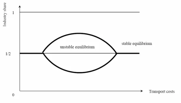
As illustrated by Figure 1, high transport costs sustain a pattern in which activities are equally split between the two regions, meaning that the share of the manufacturing sector is 1/2 in each region. At the other extreme of the spectrum, low transport costs foster the agglomeration of activities within a single region, hence implying that the share is either 0 or 1. For intermediate values, both configurations are stable equilibria, in which case the actual spatial pattern heavily depends on history. Those spatial patterns of production, as well as the conditions under which they emerge, provide a crude, but accurate, description of the general trends summarized in section 2.
Figure 1. Transport costs and industry share when labor is mobile
Thus, the mobility of labor exacerbates the general tendencies uncovered in sub-section 3.2, the reason being that the size of local markets changes with labor migration. For such self-reinforcing changes to occur, it must be that trading between regions becomes sufficiently cheap. Putting all these results together shows that lowering transport costs first leaves the location of economic activity unchanged, and then gives rise to a snowball effect that stops only when an extreme form of economic agglomeration is obtained.
One important implication of the cumulative causation triggered by the interplay of agglomeration and dispersion forces is the emergence of what can be called putty-clay geography. Even though firms are a priori footloose, once the agglomeration process is set into motion, it keeps developing within the same region. Individual choices become more rigid because of the self-reinforcing nature of the agglomeration mechanism (the snowball effect mentioned above). In other words, the process of agglomeration sparks a lock-in effect. Hence, although firms and workers are (almost) freed from natural constraints, they are still connected through more complex networks of interactions, which are more difficult to unearth than the standard location factors related to the supply of natural resources.
3.4 A welfare analysis of the core-periphery model
Whether there is too much or too little agglomeration is an issue that has never been in short supply and it is fair to say that this is one of the main questions that policy-makers would like to address. The core-periphery model shows that migration is not necessarily a force pushing for the equalization of standards of living. It may just as well reduce gaps in welfare levels as exacerbate regional disparities. Besides the standard inefficiencies generated by firms pricing above marginal costs, Krugman’s model contains new sources of inefficiency stemming from agents’ mobility. Firms and workers move without taking into account the benefits and losses they generate for both the host and departure regions. Accordingly, if it is reasonable to expect the market outcome to be inefficient, there is a priori no general indication as to the social desirability of agglomeration or dispersion.
Before proceeding, a warning is in order: both the planner seeking to maximize global efficiency and the market work with the same agglomeration and dispersion forces. Since the planning optimum and the market equilibrium depend on the fundamental characteristics of the economy, the agglomeration and dispersion forces discussed above are to be taken into account in both cases. What makes the two solutions different is the institutional mechanism used to solve the trade-off between these forces. Such a difference is often poorly understood, thus leading the public and some policy-makers to believe that the socially optimal pattern of activities has nothing to do with what the free play of market forces yields. In particular, agglomeration may be socially efficient. This is so when transport costs are sufficiently low. The reason is simple to grasp: firms are able to take advantage of the larger market created by their concentration to exploit scale economies, while guaranteeing the inhabitants of the periphery a good access to their products.
Unfortunately, welfare analyses do not deliver a simple and unambiguous message about the equilibrium spatial pattern of economic activity in the core-periphery model. Neither of the two possible equilibria - agglomeration or dispersion - Pareto dominates the other, because farmers living in the periphery always prefer dispersion, whereas farmers and workers living in the core always prefer agglomeration. In order to
compare these two market outcomes, Charlot et al. (2006) use compensation mechanisms put forward in public economics to evaluate the social desirability of a move, using market prices and equilibrium wages to compute the compensations to be paid either by those who gain from the move (Kaldor), or by those who would be hurt by the move (Hicks). They show that, once transport costs are sufficiently low, agglomeration is preferred to dispersion in that farmers and workers in the core can compensate farmers staying in the periphery. However, the latter are unable to compensate farmers and workers who would choose to form what becomes the core. This implies that none of the two configurations is preferred to the other with respect to the two criteria. Such indeterminacy may be viewed as the "resolution" of the much contrasted views that prevail in a domain in which the two tenets have many good reasons to be right.
This indeterminacy may be resolved by resorting to specific social welfare functions. Charlot et al. consider the CES family that encapsulates different attitudes toward inequality across individuals, and includes the utilitarian and Rawlsian criteria as polar cases. As expected, the relative merits of agglomeration then critically depend on societal values. If society does not care much about inequality across individuals, agglomeration (respectively, dispersion) is socially desirable once transport costs are below (respectively, above) some threshold, the value of which depends on the fundamental parameters of the economy. Even though these results are derived from social preferences defined on individualistic utilities, it is worth noting that they lead to policy recommendations that can be regarded as being region-based. This is because the market yields much contrasted distributions of income in the core-periphery structure, which correspond to equally contrasted distributions of skills between regions, as illustrated by Duranton and Monastiriotis (2002) for England, and by Combes et al. (2008a) for France.
When individual preferences are quasi-linear, one may go one step further because the total surplus is measured by the sum of individual utilities across regions and groups of workers. In this case, it is possible to determine some clear-cut and suggestive results (Ottaviano and Thisse, 2002). First, workers do not necessarily benefit from their concentration into a single region. Indeed, as said above, they do not account for the impact of their migration on their collective welfare, which typically differs from their individual welfare. This difference arises, on the one hand, because of the intensified competition that affects prices and wages and, on the other, because of the larger size of the regional markets for both products and labor. The net effect is, therefore, a priori undetermined. It has been shown, however, that the net effect is negative when transport costs take intermediate values. This is so because agglomeration leads to very low prices, whence very low wages, thus implying that the collective gains associated with agglomeration do not permit any compensation for the resulting social losses. By contrast, when transport costs are very low, both the market solution and the social optimum involve the agglomeration of the manufactured sector. This means that the total surplus is high enough for everyone in the core and the periphery to be better off.
Of course, for this to arise, interregional transfers from the core to the periphery are to be implemented.
This is not the end of the story, however. Once local interactions and knowledge spillovers among firms are taken into account, the market outcome is likely to exhibit under-agglomeration for a wider range of transport cost values (Belleflamme et al., 2000).8 Although the process of interaction goes both ways, firms worry only about their role as "receivers" but tend to neglect the fact that they are also "transmitters" to the others. Furthermore, at the optimum, prices are set at the marginal cost level, while locations are chosen so as to maximize the difference between the benefits of agglomeration and total transport costs. By contrast, at the market outcome, firms take advantage of their spatial separation to relax price competition and, whence, to make higher profits. These interactions yield clusters that are too small from the social point of view. In a setting involving a housing market, this result is confirmed by Pflüger and Südekum (2008) who show that there is under-agglomeration for low trade costs (see also Helpman, 2000).
3.5 A growth approach to regional disparities
One may wonder what the implications of the core-periphery model become once we allow the manufacturing sector to expand through the entry of new firms and a larger number of varieties. The main question is now to figure out how growth and location affect each other. More precisely, do regional discrepancies widen or fall over time, and what are the main reasons for such an evolution? To answer these questions, the core-periphery model is grafted onto an endogenous growth model involving an R&D sector, such as those developed in Grossman and Helpman (1991).
The R&D sector uses workers as its sole input to produce patents that manufacturing firms must buy to enter the product market. The price of a patent is the equivalent of the firms’ fixed production cost in the core-periphery model. Hence, the number of manufacturing firms is now variable. Farmers can work indifferently in the agricultural or manufacturing sectors, where they are paid the same wage. Although the frame of reference remains very much the same as in the core-periphery model, new issues arise because workers are free to move back and forth between regions over time, thus changing the location of the R&D sector.
Fujita and Thisse (2002) show that, at the steady-state, the spatial distribution of the R&D sector remains the same over time while the total number of patents/varieties/firms grows at a constant rate. The growth rate is measured by the variation in the number of varieties and changes with the spatial distribution of workers. In other words, the growth of the global economy depends on i s spatial t
8
Note, however, that the progressive decrease of communication costs is likely to spread the extent of spillovers, thus leading local interactions to become regional in nature.
organization. When patents can be used indifferently in either region, the market outcome is such that the entire R&D activity is always concentrated into a single region. Furthermore, the manufacturing sector is fully or partially agglomerated in the same region as the R&D sector, depending on the level of transport costs. Thus, the existence of a R&D sector is a strong agglomeration force, which magnifies the circular causation pinned down in the core-periphery model.
This result gives credence to the existence of a trade-off between growth and spatial equity. However, unlike what the analysis of the core-periphery model suggests, the welfare analysis performed by Fujita and Thisse supports the idea that the additional growth spurred by agglomeration may lead to a Pareto-dominant outcome. Specifically, when the economy moves from dispersion to agglomeration, innovation follows a faster pace. As a consequence, even those who stay put in the periphery are better off than under dispersion, provided that the growth effect triggered by agglomeration is strong enough. It is worth stressing here that this Pareto-dominance property does not require any interregional transfers: It is a pure effect of market interaction.
Clearly, the farmers living in the core of the economy enjoy a higher level of welfare than those in the periphery. Yet, even though agglomeration generates more growth and makes everybody better off, the gap enlarges between the core and the periphery. Hence, agglomeration gives rise to regressive effects in terms of spatial equity, one region being much richer than the other. Such widening welfare gaps may call for corrective policies, but such policies might in turn hurt growth and, thus, individual welfare. Note, finally, that regional income discrepancies again reflect the spatial distribution of jobs and skills. Core and periphery welfares diverge because faster growth generates additional gains that the R&D sector is able to spur by being agglomerated.
4. The bell-shaped curve of spatial development
4.1 Imperfect labor mobility
In the foregoing section, workers are assumed to have the same preferences. Although this assumption is not uncommon in economic modeling, it is highly implausible that all potentially mobile individuals will react in the same way to a given "economic gap" between regions. Some people show a high degree of attachment to the region where they are born; they will stay put even though they may guarantee to themselves higher living standards in another region. In the same spirit, lifetime considerations such as marriage, divorce and the like play an important role in the decision to migrate (Greenwood, 1997). Note, finally, that regions are not similar and exhibit different natural and cultural features, whereas people value differently local and cultural amenities. Typically, individuals exhibit idiosyncratic tastes about such attributes, so that non-economic considerations matter to potentially mobile workers when they make
their decision to move or not. In particular, as argued in hedonic models of migration, once individual welfare levels get sufficiently high through the steady increase of income, workers tend to pay more attention to the non-market attributes of their environment (Knapp and Graves, 1989).
Although individual motivations are difficult to model because they are many and often non-observable, it turns out to be possible to identify their aggregate impact on the spatial distribution of economic activities by using discrete choice theory, which aims at predicting the aggregate behavior of individuals facing mutually exclusive choices (Anderson et al., 1992; Train, 2003). In other words, a discrete choice model can be used to capture the aggregate matching between individuals and regions.9 Building on this idea, Tabuchi and Thisse (2002) have combined the core-periphery model of section 3.2 with the logit model of discrete choice theory in order to assess the impact of heterogeneity in migration behavior. In such a context, interregional migrations become sluggish, which in turn generates a very different global pattern: the industry displays a smooth bell-shaped curve of spatial development.
Figure 2. Transport costs and industry share when labor is imperfectly mobile As transport costs steadily decline, more and more firms get agglomerated in one region for the reasons explained in sub-section 3.2, but the agglomeration process is now gradual and smooth. However, full agglomeration never arises because some workers have a very good match with their region of origin and choose not to migrate.
9
It is worth mentioning that such a modeling strategy agrees with the rich body of literature, known as spatial interaction theory, which has been developed by geographers and transport analysts (Wilson, 1970; Anas, 1983). Indeed, besides workers’ location choices, trade flows also obey a structure akin to this theory as they are generated by consumers who have a preference for variety. Thus, the kind of approach proposed here reconciles different approaches developed in economic geography within a unified framework.
After having reached a peak, the manufacturing sector gradually gets re-dispersed. This is because the non-economic factors that drive the choice of a residential location become predominant and take over the economic forces stressed by NEG, the intensity of which decreases with falling transport costs. As a result, the relationship between the degree of spatial concentration and the level of transport costs is bell-shaped (see Figure 2 for an illustration). Furthermore, the domain over which this curve develops shrinks as the population becomes more heterogeneous, confirming once more the importance of the type of labor mobility. Therefore, idiosyncratic factors in migration decisions act as a strong dispersion force and change the global pattern of location decisions into a bell-shaped curve.
4.2 The role of non-tradable goods
Tradable goods do not account for a very large fraction of the GDP of developed countries. On the contrary, many consumption goods and services are produced locally and not traded between regions. The forces pushing toward factor price equalization within every region thus lead to additional costs generated by the agglomeration of firms and workers within the same region. This in turn increases the cost of living in the large region and may induce some workers to change place. A natural way to capture this phenomenon is to focus on the land market where competition gets tougher, hence the land rent rises, as more people establish themselves in the same area. Indeed, as argued in urban economics, a growing flow of workers makes commuting and housing costs higher in the city that accommodates the new comers (Fujita, 1989).
When firms set up within a central business district, workers distribute themselves around this center and commute on a daily basis. Competition for land generates a land rent whose value decreases as the distance to the employment center rises. This implies that, both the land rent and the average commuting cost are shifted upward when more workers reside in the city. Eventually, as the population keeps rising, the costs borne by workers within the agglomeration become too high to be compensated by a better access to the array of tradable goods. Therefore, dispersion arises once shipping costs have reached a sufficiently low level by comparison with commuting costs (Tabuchi, 1998; Ottaviano et al., 2002). Lower urban costs in the periphery more than offset the additional transport costs to be paid for consuming the varieties produced in the other region. Consequently, as transport costs fall, the economy involves dispersion, agglomeration, and re-dispersion. This is strikingly similar to what we have seen in sub-section 4.1, but what triggers the re-dispersion of workers is now the crowding of the land market.10
Two final comments are in order. First, the redispersion process across regions depends on the efficiency of urban transport infrastructures, thus showing why urban and 10
Negative externalities arising in the urban agglomeration, such as transport congestion, pollution and a high crime rate, play a similar role and speed up the re-dispersion of activities toward less crowded regions.
interregional transport policies should be coordinated. If commuting costs are low (respectively, high), the agglomeration will remain the equilibrium outcome for a wider (respectively, narrower) range of transport cost values, as illustrated by the emergence of large polycentric metropolises in the US (Anas et al. 1998). The relocation of manufactured activities away from large metropolitan areas toward medium-sized cities provides an example of the impact that high commuting costs may have on firms’ locations (Henderson, 1997). Second, the burden of urban costs may be alleviated when
secondary employment centers are created. Such a morphological change in the urban structure, which makes the city polycentric, slows down the re-dispersion process and allows the agglomeration to maintain, at least to a large extent, its supremacy (Cavailhès et al., 2007). This draws attention to two facts that transport analysts often neglect: on the one hand, the local mobility of people (i.e. commuting) may affect the global organization of the economy and, on the other hand, the global mobility of commodities is likely to have an impact on the local organization of production and employment.
4.3 Vertical linkages
So far in the analysis, agglomeration is driven by the endogeneity of the size of local markets caused by the mobility of consumers/workers. When labor is immobile across regions but mobile between sectors, the cumulative causation falls short and the symmetric equilibrium is the only stable outcome. However, another reason for the market size to be endogenous is the presence of input-output linkages between firms:
what is an output for a firm is an input for another. Intermediate production represents a big share of the industrial output. For example, in the United States, intermediate consumption of goods accounted for almost 69% of the total production manufactured in 1997. Besides the standard competition effect, the entry of a new firm in a region also increases the market size of upstream firms-suppliers (market size effect) and decreases the costs of downstream firms-customers (cost effect). In such a context, the agglomeration of the final and intermediate sectors in a particular region may occur because firms want to be close to their customers or suppliers.
This alternative setting allows one to shed light on two new forces that are likely to play a major role in the evolution of the space-economy (Krugman and Venables, 1995). When more firms are concentrated in a region where the supply of labor is totally inelastic, they will end up paying higher wages to their workers if the size of the two industrial sectors becomes large. This has two opposing effects for the core region. On the one hand, the final demand in this region increases because consumers enjoy higher incomes there. We find again a force of agglomeration linked to final demand, as in Krugman. However, this is no longer triggered by an increase in the size of the population, but by an increase in individual incomes. On the other hand, the same phenomenon generates a force of dispersion, which feeds the fear of de-industrialization, that is, the high labor costs that prevail in the core. If wages are much lower in the periphery, beyond some level of integration, firms will find it profitable to relocate there, even if the demand for their product is lower than in the
core. In doing so, they have the possibility to produce at lower costs while keeping a very good access to the core region.11
Thus, if the impact of economic integration highlighted in section 3 - namely, the strengthening of regional inequalities - continues to appear up to a certain level of integration, the inverse process is set in motion beyond this level, thus showing that the pursuit of economic integration contributes to a decrease in regional inequalities. We therefore find a re-industrialization of the periphery and even a possible, and simultaneous, de-industrialization of the core. This new phenomenon of regional convergence, which arises here for very high degrees of integration, concurs with the prediction that re-equilibrating forces in favor of peripheral zones come into play once transport costs have reached a sufficiently low level. The relocation of some activities in the new Member States of the European Union seems to confirm the plausibility of such an evolution (Brülhart, 2006).
4.4 The spatial fragmentation of firms
A growing number of firms choose to break down their production process into various stages spread across different regions. Specifically, the modern firm organizes and performs discrete activities in distinct locations, which altogether form a supply chain
starting at the conception of the product and ending at its delivery. This spatial fragmentation of production aims at taking advantage of differences in technologies, factor endowments, or factor prices across places (Feenstra, 1998; Spulber, 2007). The most commonly observed pattern is such that firms re-locate their production activities in low-wage regions or countries, while keeping their strategic functions (e.g. management, R&D, marketing and finance) concentrated in a few affluent urban regions where the high-skilled workers they need are available.
In such a context, the development of new communication technologies is a major force that should be accounted for. It goes hand in hand with the growing role of transportation firms in the global logistics. With this in mind, two types of spatial costs must then be considered, namely communication costs and transport costs. Low transport costs allow firms producing overseas to sell their output on their home market at a low price. Equally important, but perhaps less recognized, is the fact that coordinating activities within a firm is more costly when headquarters and plant are physically separated because the transmission of information remains incomplete and imperfect (Leamer and Storper, 2001). However, lower communication costs make coordination easier and, therefore, facilitate the process of fragmentation. More precisely, in order to make low-wage areas more attractive for the establishment of their production, firms need both the development of new communication technologies and substantial decreases in transport costs.
11
Assume that each firm has two units, one headquarter and one plant. All headquarters are located in the same region and use skilled labor, whereas plants use headquarter-services together with unskilled labor. A firm is free to decentralize its production overseas by choosing distinct locations for its plant and headquarter. Apart from this change, the framework used is the same as in sub-section 3.2. Two main scenarios are to be distinguished as they lead to very different patterns (Fujita and Thisse, 2006). When communication costs are sufficiently high, all firms are national and established in the core region. Once communication costs steadily decrease, the industry moves toward a configuration in which some firms become multinational whereas others remain national. Eventually, when these costs have reached a sufficiently low level, the economy ends up with a de-industrialized core that retains only firms' strategic functions.
A fall in transport costs may lead to fairly contrasted patterns of production. In particular, two scenarios are to be considered. When communication costs are high, reducing transport costs leads to a growing agglomeration of plants within the core, very much as in the core-periphery model. However, the agglomeration process is here gradual instead of exhibiting a bang-bang behavior. Things are totally different when communication costs are low. For high transport costs, most plants are still located within the core region. However, once these costs fall below some threshold, the re-location process unfolds over a small range of transport cost values. This could explain why the process of de-industrialization of some developed regions seems, first, to be slow and, then, to proceed quickly, yielding a space-economy very different from the initial one.12
In a related context, Robert-Nicoud (2008) stresses a different aspect of the fragmentation process, which allows firms to simultaneously reap the benefit of agglomeration economies in the core regions and of low wages in the periphery. Specifically, the reduction of employment in some routine tasks in rich regions helps sustain and reinforce employment in the core competencies of firms in such regions. Consequently, the loss of some (unskilled) jobs permits to retain firms’ “core competencies” in the core regions as well as the corresponding (skilled) jobs. By contrast, preventing firms to outsource abroad their routine tasks is likely to induce them to relocate their entire activities in the periphery, thus destroying all jobs in what was the core.
Thus, by facilitating the vertical disintegration of firms, lower communication costs are likely to have a deep impact on the structure of employment in developed countries. It should be clear that the interaction between communication costs and transport costs has become a critical issue for the future of the space-economy.
12
The re-dispersion of firms, which occurs through their fragmentation, rests on the existence of sufficiently strong interregional wage differentials. Any force that narrows down the wage gap thus thwarts the re-dispersion of firms and, consequently, contributes to maintain the core-periphery structure (Faini, 1999).
5. How to measure transport costs and their impact on the
distribution of activities?
In NEG models, the transport sector is a silent sector. To a large extent, this is because economists have a fairly simplistic view of transport costs, which leads them to disregard several important dimensions stressed by transportation economists (Rietveld and Vickerman, 2004). Yet, such measures are crucial when we come to the evaluation of the impact of lowering transport costs on the spatial distribution of activities in real-world economies.
5.1 The measurement of transport costs
Most NEG models build on the standard iceberg formulation of transport costs. Albeit popularized by Samuelson (1954), the iceberg frame goes back to von Thünen (1826) who argued that transport costs would be given by the amount of grains consumed by horses pulling the loaded carriages. In line with this metaphor, most NEG models rest on the assumption that moving commodities incurs the loss of a given share of the load. Modeling transport costs as if goods were truly “melting” en route is a convenient analytical device that circumvents the need to consider the transport sector per se and its related interactions with other markets. More precisely, the iceberg formulation implies that transport costs are multiplicative to the “free-on-board” (FOB) price of products, so that any increase in this price raises freight charges proportionally. Conversely, any increase in the iceberg cost translates into a larger delivered or “cost-insurance-freight” (CIF) price. Denoting by p the FOB price and by p* the CIF price, the freight rate is
τ
= p* p−1.In that spirit, the first generation of NEG empirics uses two series of transport cost proxies. The first one is the share of GDP spent in transport activities. In the US, Glaeser and Kohlhase (2004) report that this share has fallen from about 10% in late nineteenth century to about 3% nowadays. Adding logistic and transport activities yields a larger share of 9.5% (Wilson, 2006).
However, the share of transport and logistic expenditures in GDP provides only a lower bound for actual transport costs because it neglects two major features. First, national accounts exclude in-house transport, which may account for up to 15% of transport activities in a country such as France. Second, a large share of GDP is not shipped across locations. Hence, the above data provides at best very crude approximations of actual transport expenditures on traded goods. It seems therefore preferable to evaluate transport costs from other sources.
Based on customs data, transport costs may be computed as the ratio between the CIF value of a traded flow reported by the importing country, which is inclusive of freight charges, and the related FOB value reported by the exporting country, which is
exclusive of these charges. The CIF/FOB transport margin is commodity-specific and varies with the origin-destination route. Unfortunately, for many countries, especially developing ones, this technique yields large inconsistencies that are mostly due to discrepancies in trade reporting techniques (Hummels and Lugovskyy, 2006).
In a few importing nations, such as New Zealand, the US or Latin America countries (Argentina, Chile, Brazil, Paraguay and Uruguay), freight expenditures are directly reported in import customs declarations. For these countries, the ratio of freight charges to import values yields a transport cost that is purged from the aforementioned inconsistencies. Building on this method, Hummels (2001) reports
considerable variation in freight rates across importers, exporting routes and goods. The US is shown to have the lowest transport costs with a 3.8% margin, which is around 4-fold that of a land-locked country such as Paraguay (13.3%). Hummels (2007) evaluates that, even for the median US good shipped, the related freight rate was nine times larger than the corresponding tariff duty in 2004. Along the same line, the Global Trade Analysis Project (GTAP), which provides one of the most disaggregated databases on import customs declarations, reports average transport margins that would range, for the US, between 0.4% (cobalt ores) and 136% (grapefruit).13 The variability across routes is also very large, the lower and upper bounds being for, respectively, the countries close to the US (Canada and Mexico) and distant trading partners such as Australia.
Nonetheless, a warning is in order regarding the use of transport margins computed from trade data. A major pitfall of this method is that freight expenditures might be low because trade strategies are designed by firms and carriers to reduce transport costs. If traders substitute away from goods or routes with relative high freight costs, the picture drawn from trade margins could be misleading, and the real average level of transport costs vastly underestimated. In addition, null flows, which remain mostly ignored in empirical analyses, probably mean that the transport costs of some goods are prohibitive. A well-known example is provided by the non-tradable goods whose share in households’ and firms’ consumption is large. One way to circumvent both the endogeneity of transport margins and its related trade composition effects is to identify the various factors that determine the absolute level of freight costs, a question to which we now move.
The cost of shipping commodities across regions depends on several variables. The most common functional form used in empirical works transport costs builds on the success story of the gravity model, which has been the workhorse of new trade theories (Feenstra, 2004). It is given by the following expression:
) , , ( 1 0 ij ij i j ij Dist f X X X t =
δ
δ (1)13 See https://www.gtap.agecon.purdue.edu/resources/download/135.pdf.
where
δ
0 is a parameter evaluating the overall efficiency of the transport sector. , is the distance between the region of origin i and the region of destination j,ij
Dist 14
δ
1a parameter measuring the inverse distance-decay effect, while is a separable function of three vectors of variables, namely the non-distance pair-specific ( ), origin-specific and destination-specific factors affecting transport costs ( and . Typical variables and their impact are described below.
f
ij
X
i
X
XjFirst, transport involves industry-specific costs, which depend on the nature and the quality of the commodity shipped. These costs are often approximated by the weight to value ratio of goods, which captures the scale effects generated by high trade volumes and the differences in both the transportability (bulk size) and the quality of goods (damage liabilities). Hummels (2001) estimates that the elasticity of the weight to value ratio is very similar to that of distance (close to 0.25), which means that doubling either the unit value of goods or the distance covered yields an increase in transport costs equal to 19% = (20.25 - 1) x 100.15 However, these elasticities significantly vary
across transport modes. For example, an additional mile is far more expensive for air (from 27% up to 43%) than for ocean freight (15%), while a marginal increase in the unit value of goods has a lower impact on road transport costs than on air or rail freight rates (Hummels, 2007). Albeit important, the weight to value ratio is difficult to observe at the interregional level or within free-trade areas and, absent data, is often non-industry specific.
ij
t
Second, whenever shipments have to cross borders, transit delays, custom inspections, changes in bulk standards or transport mode switching involve additional charges. Once again, absent data, such losses are often captured by a dummy equal to one if i and j are separated by a border and to zero otherwise. Conversely, trade may be facilitated by international agreements, technological progress, transit infrastructure, integrated transport networks (for instance between neighboring countries), or smooth geography. For instance, Limão and Venables (2001) consider adjacency (a dummy indicating whether i and j have a common border), landlockness (two dummies indicating whether i
and j do not have access to the sea), insularity (two dummies indicating whether i and j
are islands), and infrastructure density (both between and within i and j). According to their estimates, in comparison with a coastal country, a landlocked country would bear an additional transport cost of 50%, which could be overcome partially by improving onshore and transit infrastructure. By improving its infrastructure from the median to the top 25th percentile, a country would save about 13% in transport costs, which would be equivalent to make it 2358km closer to its trading partners. Micco and Serebrisky
14
At the level of macro-regions, it usually refers to the geodesic distance between the main cities of the origin and destination regions.
15
Note also that, quite unexpectedly, physical distance does not only matter for commodity flows. Blum and Goldberg (2006) find that, for taste-dependent differentiated digital products (such as music or electronic games), a 1% increase in distance reduces the number of websites visits by 3.25%, once controlled for key other determinants such as language or internet penetration.