HAL Id: tel-02406953
https://hal.archives-ouvertes.fr/tel-02406953v2
Submitted on 26 Jun 2020HAL is a multi-disciplinary open access
archive for the deposit and dissemination of sci-entific research documents, whether they are pub-lished or not. The documents may come from teaching and research institutions in France or abroad, or from public or private research centers.
L’archive ouverte pluridisciplinaire HAL, est destinée au dépôt et à la diffusion de documents scientifiques de niveau recherche, publiés ou non, émanant des établissements d’enseignement et de recherche français ou étrangers, des laboratoires publics ou privés.
an explicitely typed lambda-calculus
Claude Stolze
To cite this version:
Claude Stolze. Combining union, intersection and dependent types in an explicitely typed lambda-calculus. Logic [math.LO]. COMUE Université Côte d’Azur (2015 - 2019), 2019. English. �NNT : 2019AZUR4104�. �tel-02406953v2�
Types union, intersection, et dépendants
dans le lambda-calcul explicitement typé
Claude STOLZE
INRIA Sophia-Antipolis Méditerranée
Présentée en vue de l’obtention du grade de docteur en Informatique de l’Université Côte d’Azur.
Dirigée par : Luigi Liquori
Soutenue le : 16 décembre 2019
Devant le jury, composé de : Giuseppe Castagna Ugo de’Liguoro Silvia Ghilezan Furio Honsell Delia Kesner Bruno Martin Jakob Rehof Luigi Liquori
Types union, intersection, et dépendants
dans le lambda-calcul explicitement typé
Jury
Président du jury
Bruno Martin, Professeur, Université Côte d’Azur Rapporteurs
Silvia Ghilezan, Professeur, University of Novi Sad, Serbie Delia Kesner, Professeur, Université de Paris
Examinateurs
Giuseppe Castagna, Directeur de recherche, CNRS, Université de Paris Ugo de’Liguoro, Professeur, Università degli Studi di Torino, Italie Furio Honsell, Professeur, Università degli Studi di Udine, Italie
Jakob Rehof, Professeur, Technische Universität Dortmund, Allemagne Encadrant
dans le lambda-calcul explicitement typé
Résumé :
Le sujet de cette thèse est sur le lambda-calcul décoré avec des types, communément appelé « calcul typé à la Church ». Nous étudions des versions de ce lambda-calcul muni de types intersections, tels que ceux décrits dans le livre « Lambda-lambda-calculus with types » de Barendregt, Dekkers et Statman ; les types unions, qui ont été introduits par Plotkin, MacQueen et Sethi ; et les types dépendants, tels qu’ils ont été décrits par Plotkin, Harper et Honsell lorsqu’ils ont introduit le Logical Framework d’Edinbourgh LF. Les types intersections et unions sont un moyen d’exprimer du polymorphisme ad hoc et sont une alternative au polymorphisme paramétrique de Girard. Les types dépendants ont été introduits pour formaliser la logique intuitionniste avec la correspondance de Curry-Howard. Le système de types obtenu peut être enrichi avec une relation de soutypage décidable. La combinaison de ces trois disciplines de type donne lieu à une famille de calculs qui peuvent être paramétrés et classifiés. Nous appelons le système générique le Delta-calcul. Nous discutons ensuite des décisions de conception qui nous ont amené à la formulation de ces calculs, nous étudions leur métathéorie, et nous présentons divers exemples d’applications avant de présenter une implémentation logicielle du Delta-calcul, avec une description des algorithmes de vérification de type, de raffinement, de soutypage, d’évaluation, ainsi que de l’interface en ligne de commande. Ce travail de recherche peut être vu comme un petit pas franchi dans la direction d’une théorie des types alternative pour définir du polymorphisme dans les langages de programmation et dans les assistants de preuve interactifs.
types in an explicitely typed lambda-calculus
Abstract:
The subject of this thesis is about lambda-calculus decorated with types, usually called “Church-style typed lambda-calculus”. We study this lambda-calculus enhanced with Intersection types, as described by Barendregt, Dekkers and Statman in the book “Lambda-calculus with Types”; Union types, as introduced by Plotkin, MacQueen and Sethi; and Dependent types, as described by Plotkin, Harper and Honsell when they introduced the Edinburgh Logical Framework LF. Intersection and union types are a way to express ad hoc polymorphism and are an alternative to the parametric polymorphism of Girard. Dependent types were introduced as a way to formalize intuitionistic logic using the “proofs-as-lambda-terms / formulae-as-types” Curry-Howard principle. The resulting type system can be enriched with a decidable subtyping relation. Combining these three type disciplines gives rise to a family of calculi that can be parametrized and classified: we call the resulting system the Delta-calculus. We then discuss the design decisions which have led us to the formulation of these calculi, study their metatheory, and provide various examples of applications; and we finally present a software implementation of the Delta-calculus, with a description of the type checker, the refinement algorithm, the subtyping algorithm, the evaluation algorithm and the command-line interface. This work can be understood as a little step toward an alternative type theory to defining polymorphic programming languages and interactive proof assistants.
Remerciements – Acknowledgements
Je ne peux commencer cette thèse sans remercier mon directeur, Luigi Liquori, pour tout le soutien et tous les conseils qu’il m’a prodigués au cours de ces trois années de travail ensemble. Merci en particulier pour la confiance que tu m’as accordé. Tu m’as appris l’exigeant métier de chercheur, notamment qu’un article n’a fini d’être écrit que lorsque la deadline est passée, et que les détails mathématiques et l’esthétique ont une importance cruciale dans la science. J’aimerais aussi remercier ma mère pour son soutien à distance de l’autre bout de la France, et qui me réconfortait quand j’avais le mal du pays. Je voudrais remercier Enrico Tassi qui m’a détaillé les entrailles du code de Coq. Et sans oublier mes camarades Siargey, Owen, Sophie, Cécile, Damien, Carsten, Giovanni, et tant d’autres.
I would also like to thank my jury for accepting to review my work. I am particularly thankful to Delia Kesner and Silvia Ghilezan, who accepted to be my referees. Many thanks to Bruno Martin, Giuseppe Castagna, Ugo de’Liguoro, Furio Honsell, and Jakob Rehof, for showing interest in my work and for accepting to participate in this jury.
Contents
1 Introduction 1
1.1 Prolegomenon . . . 1
1.2 Contributions . . . 3
1.3 Related works . . . 5
2 A typed calculus with intersection types 9 2.1 Syntax, Reduction and Types . . . 10
2.1.1 The ∆-calculi . . . 11
2.1.2 The ∆-chair . . . 14
2.2 Examples . . . 15
2.2.1 On synchronization and subject reduction . . . 18
2.3 Metatheory of ∆T R . . . 19
2.3.1 General properties . . . 19
2.3.2 Synchronous reduction . . . 25
2.3.3 Strong normalization of the generic ∆-calculus . . . 29
2.4 Church-style vs. Curry-style λ-calculus . . . 31
2.4.1 Relation between type assignment systems λT ∩ and typed systems ∆ T R 31 2.4.2 Subtyping and explicit coercions . . . 34
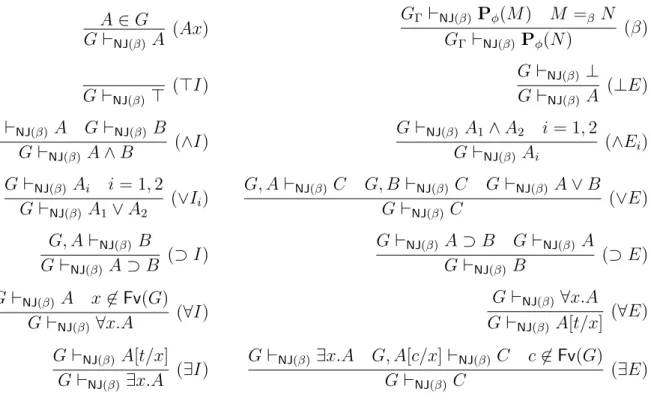
3 Adding union types 39 3.1 Syntax and semantics of ∆BDdL and λ@BDdL . . . 40 3.2 Metatheory of ∆BDdL and λ@BDdL . . . 43 4 On Mints’ realizability 45 4.1 Presentation of NJ(β) . . . 46 4.2 Soundness of NJ(β) . . . 47 4.3 Completeness of NJ(β) . . . 49
4.3.1 Failure of completeness of NJ(β) without subtyping . . . 49
4.3.2 Counter-example . . . 50
5 Subtyping algorithm 51 5.1 The algorithm, shortly explained . . . 51
5.1.1 Soundness and correctness of the algorithm . . . 54
5.2 Coq implementation of the theory Ξ . . . 55
5.2.1 Definition of normal forms . . . 57
5.2.2 Filters and ideals . . . 59 xi
5.2.3 Induction scheme for filters and ideals . . . 60
5.2.4 Properties of filters and ideals . . . 62
5.3 Coq implementation of the subtyping algorithm . . . 63
5.4 Extracting the subtyping algorithm in OCaml . . . 69
5.5 The preorder tactic . . . 70
5.5.1 Denotation . . . 71
5.5.2 Implementation of the heuristic function . . . 72
5.5.3 Reification . . . 74
6 Dependent types 77 6.1 The ∆-framework: LF with proof-functional operators . . . 80
6.2 Relating LF∆ to λBDdL . . . 84
6.2.1 Typed derivation of Pierce’s example . . . 85
6.2.2 LF∆ metatheory . . . 86
6.3 Minimal relevant implications and type inclusion . . . 89
6.4 Pure Type System presentation of LF∆ . . . 91
6.5 Future Work . . . 92
7 Implementation of the theorem prover Bull 95 7.1 de Bruijn indices in Bull . . . 96
7.2 Syntax of terms . . . 97
7.2.1 Concrete syntax . . . 98
7.2.2 Implementation of the syntax . . . 99
7.2.3 Environments . . . 100
7.2.4 Suspended substitution . . . 101
7.3 The evaluator of Bull . . . 102
7.3.1 Reduction rules . . . 102
7.3.2 Implementation . . . 102
7.4 The subtyping algorithm of Bull . . . 104
7.5 The unification algorithm of Bull . . . 105
7.6 The refinement algorithm of Bull . . . 105
7.7 The Read-Eval-Print-Loop of Bull . . . 108
7.8 Future work . . . 109
8 Examples in Bull 115 8.1 Encodings in LF∆ . . . 115
8.1.1 Pierce’s code . . . 116
8.1.2 Hereditary Harrop formulæ . . . 116
8.1.3 Natural deductions in normal form . . . 118
List of Figures
1.1 Pierce’s code . . . 7
2.1 Minimal type theory 6min, axioms and rule schemes (from Figure 13.2 and 13.3 of [12]) . . . 10
2.2 Generic intersection type assignment system λT ∩ (from Figure 13.8 of [12]) . 10 2.3 Type theories λCD ∩ , λCDS∩ , λCDV∩ , and λBCD∩ . The “ref.” column refers to the original articles these theories come from . . . 11
2.4 Generic ∆-calculus ∆T R . . . 13
2.5 Generic intersection typed system λ@T R . . . 14
2.6 The ∆-chair . . . 15
2.7 On the left: source systems. On the right: target systems without the (6T) rule . . . 37
3.1 Intersection and union type assignment system λBDdL [7] . . . . 40
3.2 Typed calculus λ@BDdL [40] . . . 41
3.3 ∆-calculus ∆BDdL . . . . 42
4.1 The logic NJ(β) . . . 46
5.1 The type theory Ξ of [7] . . . 52
6.1 The type assignment system λBDdL of [7] and the type theory Ξ . . . . 79
6.2 The syntax of the ∆-framework . . . 80
6.3 The extended essence function . . . 81
6.4 The reduction semantics . . . 81
6.5 Valid signatures and contexts . . . 82
6.6 Valid kinds and families . . . 83
6.7 The type rules for valid objects . . . 83
6.8 Encoding of Ω . . . 84
6.9 Pierce’s one-step reduction counter-example . . . 84
6.10 The forgetful mappings || − || and | − | . . . 87
6.11 The coercion function . . . 90
6.12 Pure Type System presentation of the ∆-framework (signature and context) 91 6.13 Pure Type System presentation of the ∆-framework (terms) . . . 92
7.1 Structural rules of the unification algorithm . . . 106
7.2 Rules for (1st part) . . . 108⇑ xiii
7.3 Rules for (2nd part) . . . 111⇑ 7.4 Rules for . . . 112F 7.5 Rules for . . . 112⇓ 7.6 Rules for E ⇑ . . . 113 7.7 Rules for E ⇓ . . . 114 8.1 The LF∆ encoding of Hereditary Harrop Formulæ . . . 117
Chapter
1
Introduction
“That logic has advanced in this sure course, even from the earliest times, is apparent from the fact that, since Aristotle, it has been unable to advance a single step and, thus, to all appearance, has reached its completion.”
Immanuel Kant, Preface to the second edition of The Critique of Pure Reason, 1787
1.1
Prolegomenon
When George Boole wrote Mathematical Analysis of Logic in 1847 [19], he modestly aimed at an algebraic clarification of Aristotelian logic, and did not immediately realize his work was the beginning of a deep change in the study of mathematics which would later trigger the foundational crisis of mathematics.
In 1903, Bertrand Russell [85], in The Principles of Mathematics1, opened a Pandora’s
box when he considered “predicates which are not predicable of themselves”2. As it is
widely known nowadays, Russell’s contradiction – a modern version of the liar’s paradox – consists of defining a predicate P (x) def= ¬x(x), and deducing both P (P ) and ¬P (P ). In order to circumvent this contradiction, Russell introduced, in the Appendix B of the same book, the Doctrine of Types:
“The doctrine of types is here put forward tentatively, as affording a possible solution of the contradiction [. . . ]. Every propositional function φ(x) – so it is contended – has, in addition to its range of truth, a range of significance, i.e. a range in which x must lie if φ(x) is to be a proposition at all, whether true or false. This is the first point in the theory of types; the second point is that ranges of significance form types, i.e. if x belongs to the range of significance of φ(x), then there is a class of objects, the type of x, all of which must also belong to the range of significance of φ(x).”
This general idea set the foundation of the (many) theories of types, which were widely developed during the course of the twentieth century. In 1934, Haskell Curry was “concerned with statements [. . . ] of the form "f is a function on X to Y "” [31]. Haskell
1Not to be confused with Principia Mathematica, which he wrote with Alfred Whitehead from 1910
to 1913.
2In Section 78, simply called “The contradiction”.
Curry, and later William Howard, discovered that rules determining that a function has some type where very similar to logical rules determining that a proof shows the validity of some proposition. The proofs-as-functions/propositions-as-types principle is now known as the Curry-Howard correspondence [58].
In short, types are a tool used to give a notion of a well-formed expression: – we can use types to describe well-formed propositions and proofs;
– we can use types to describe well-formed computable functions.
Among the most impactful developments from the previous century of type theory as a foundation for mathematics, we can cite Automath by N. G. de Bruijn [34], the first theorem prover, whose development started in the sixties, the intuitionistic type theory of Per Martin-Löf [69], and finally the Calculus of (Inductive) Constructions by Thierry Coquand, Gérard Huet [30], Frank Pfenning, and Christine Paulin-Mohring [76], which is the theoretical foundation of the Coq theorem prover [36].
The model of computation which is the most associated with type theory is the λ-calculus, this language developed by Alonzo Church in the thirties. The pure λ-calculus has two basic operations:
1. the first one is application, simply noted with a space: the expression M N denotes the function M applied to its argument N ;
2. the second one is λ-abstraction, noted with the binder λ: the expression λx.M denotes a function taking x as an argument and returning the expression M (possibly containing occurrences of x).
We can see λ-abstraction as a function constructor, and application as a function elimi-nator. Combining λ-abstraction and application gives two computational rules:
(β) (λx.M ) N reduces to M [N/x], i.e. all the free occurrences of x in M are substituted by N . This is the elimination of the construction of a function, and it is called a β-reduction;
(η) λx.M x reduces to M if x is not free in M . This is the construction of the elimination of a function, and it is called an η-reduction.
We can also assign type to terms. Intuitively:
– in the λ-calculus à la Curry: we assign a type to a pure λ-term. For the simply-typed λ-calculus, we get the following rules for λ-abstraction and application:
Γ, x:σ ` M : τ
Γ ` λx.M : σ → τ (→I)
Γ ` M : σ → τ Γ ` N : σ
Γ ` M N : τ (→E)
As you can see, stating that M has σ → τ intuitively means that M is a function on σ to τ ;
– in the calculus à la Church: we decorate a term with types, typically the λ-abstraction becomes λx:σ.M , where we explicitly state that x has type σ. For the simply-typed λ-calculus, we get the following rules for λ-abstraction and application:
Γ, x:σ ` M : τ
Γ ` λx:σ.M : σ → τ (→I)
Γ ` M : σ → τ Γ ` N : σ
Among the many type systems for the λ-calculi, intersection is an interesting connec-tive (see Henk Barendregt, Wil Dekkers, and Richard Statman [12] : intuiconnec-tively, if some term M has both type σ and type τ , then we say it is polymorphic and it has type σ ∩ τ , as the derivation rules show:
Γ ` M : σ Γ ` M : τ Γ ` M : σ ∩ τ (∩I) Γ ` M : σ ∩ τ Γ ` M : σ (∩E1) Γ ` M : σ ∩ τ Γ ` M : τ (∩E2) The dual connective of intersection, namely union (see David MacQueen, Gordon Plotkin, and Ravi Sethi [68]), states that if M has type σ or τ , then it has type σ ∪ τ , as the derivation rules show:
Γ ` M : σ Γ ` M : σ ∪ τ (∪I1) Γ ` M : τ Γ ` M : σ ∪ τ (∪I2) Γ, x:σ ` M : ρ Γ, x:τ ` M : ρ Γ ` N : σ ∪ τ Γ ` M [N/x] : ρ (∪E)
1.2
Contributions
The subject of this thesis is to study intersection and union types in λ-calculi à la Church, with two goals:
1. finding a λ-calculus à la Church with intersection and union types which is faithful to the corresponding pure λ-calculi à la Curry;
2. conceiving and implementing a logical framework based on intersection and union types.
Building a λ-calculus à la Church with intersection and union types
Designing a λ-calculus à la Church with intersection and union types is challenging. The usual approach of simply adding types to binders does not work, as shown here:
x:σ ` x:σ (Var) ` λx:σ.x:σ → σ (→I)
x:τ ` x:τ (Var) ` λx:τ.x:τ → τ (→I)
` λx:???.x:(σ → σ) ∩ (τ → τ ) (∩I)
Same difficulties can be found with union types. In this thesis we propose a solution to this challenge by designing a λ-calculus à la Church, called the ∆-calculus (see Chapters 2 and 3). In a nutshell: each term of the ∆-calculus has a corresponding pure λ-term, called its essence. Intersection types are constructed with strong pairs, a cartesian pair which ensures both its components share the same essence. Dually, union types are constructed with strong sums, whose original feature is that it ensures both cases of its elimination share the same essence.
Building a logical framework based on intersection and union types
We have designed a logical framework based on proof-functional logic (see Chapter 6), and using dependent types as in the Edinburgh Logical Framework [52]. In a nutshell:
- Strong disjunction is a proof-functional connective that can be interpreted as the union type ∪ [39, 88]: it contrasts with the intuitionistic connective ∨. As Pottinger [80] did for intersection, we could say that asserting (A ∪ B) ⊃ C is to assert that one has a
reason for (A ∪ B) ⊃ C, which is also a reason to assert A ⊃ C and B ⊃ C. A simple example of a logical theorem involving intuitionistic disjunction which does not hold for strong disjunction is ((A ⊃ B) ∪ B) ⊃ A ⊃ B. Otherwise there would exist a term which behaves both as I and as K.
- Strong (relevant) implication is yet another proof-functional connective that was interpreted in [8] as a relevant arrow type →r. As explained in [8], it can be viewed as
a special case of implication whose related function space is the simplest one, namely the one containing only the identity function. Because the operators ⊃ and →r differ,
A →r B →r A is not derivable.
- Dependent types, as introduced in the Edinburgh Logical Framework [52] by Robert Harper, Furio Honsell, and Gordon Plotkin, allows considering proofs as first-class citi-zens, albeit differently, with respect to proof-functional logics. The interaction of both dependent and proof-functional operators is intriguing. Their combination opens up new possibilities of formal reasoning on proof-theoretic semantics.
We have also implemented a prototype of an interactive theorem prover based on this logical framework, called Bull. For instance, the following code snippet shows the implementation of a polymorphic identity on A and B, using a strong pair, which ensures
that id1 and id2 have the same essence.
Definitionpoly_id : (A −>A) & (B −>B) := let id1 x := xin
let id2 x := xin < id1, id2 >.
Organization of this thesis This thesis is organized as follows:
- Chapter 2 presents a generic ∆-calculus, i.e. a generic typed λ-calculus with inter-section types. We study some of its instances and their properties, as well as their relation with standard λ-calculus with intersection types;
- Chapter 3 extends the previous ∆-calculus with union types, and defines a typed λ-calculus λ@BDdL
, and recalls the original λ-calculus [7] these new systems are inspired from;
- Chapter 4 sketches the logical interpretation of intersection and union types. More precisely, we define an interpretation of typing judgments M : σ into a first-order logical proposition rσ[M ] in the logic NJ(β);
- Chapter 5 defines a subtyping algorithm for intersection and union types. This algorithm is then fully implemented and certified in Coq. We detail the Coq imple-mentation;
- Chapter 6 extends the ∆-calculus by adding dependent types, in the style of the Edinburgh Logical Framework (LF). We call the resulting system the ∆-framework LF∆, and we prove its metatheoretical properties;
- Chapter 7 presents an OCaml implementation of the ∆-framework into an inter-active theorem prover, called Bull. The technical details of the implementation (syntax, semantics, typechecking, and Read-Eval-Print loop) are described;
- Chapter 8 presents some examples of encodings in the ∆-framework, as well as their implementation in Bull.
Publications
During the course of my thesis, I published the following conference papers:
– Luigi Liquori and Claude Stolze. The Delta-calculus: Syntax and Types. In 4th International Conference on Formal Structures for Computation and Deduction, FSCD 2019, pages 28:1–28:20. Schloss Dagstuhl-Leibniz-Zentrum fuer Informatik, June 2019. [66]
– Furio Honsell, Luigi Liquori, Ivan Scagnetto, and Claude Stolze. The Delta-framework. In 38th IARCS Annual Conference on Foundations of Software Technology and Theoretical Computer Science, FSTTCS 2018, pages 37:1–37:21. Schloss Dagstuhl-Leibniz-Zentrum fuer Informatik, December 2018. [57]
– Luigi Liquori and Claude Stolze. A Decidable Subtyping Logic for Intersection and Union Types. In 2nd International Conference on Topics in Theoretical Computer Science, TTCS 2017, pages 74–90. Springer, September 2017. [65]
– Claude Stolze, Luigi Liquori, Furio Honsell, and Ivan Scagnetto. Towards a Logical Framework with Intersection and Union Types. In 11th International Workshop on Logical Frameworks and Meta-languages, LFMTP 2017, pages 1–9. ACM, Septem-ber 2017. [88]
– Daniel J. Dougherty, Ugo de’Liguoro, Luigi Liquori, and Claude Stolze. A Realiz-ability Interpretation for Intersection and Union Types. In Programming Languages and Systems – 14th Asian Symposium, APLAS 2016, pages 187–205. Springer, Oc-tober 2016. [39]
Software
During the course of my thesis, I developed a prototype of an interactive theorem prover implementing the ∆-framework, called Bull [87].
1.3
Related works
In order to foster the imagination of the reader about the topic we will study in this thesis, we shortly present works related to our field of interest.
λ-calculi with intersection types à la Curry
Intersection type theories T were first introduced as a form of ad hoc polymorphism in (pure) λ-calculi à la Curry. The paper by Barendregt, Coppo, and Dezani [11] is a classic reference, while [12] is a definitive reference.
Intersection type assignment systems λT
∩ have been well-known in the literature for
almost 40 years for many reasons: among them, characterization of strongly normalizing λ-terms [12], λ-models [4], automatic type inference [60], type inhabitation [92, 82], type unification [43]. As intersection had its classical development for type assignment systems,
many papers tried to find an explicitly typed λ-calculus à la Church corresponding to the original intersection type assignment systems à la Curry. The programming language Forsythe, by Reynolds [83], is probably the first reference, while Pierce’s Ph.D. thesis [77] combines also unions, intersections and bounded polymorphism. Wells et al. [95] use intersection types as a foundation for typed intermediate languages for optimizing compilers for higher-order polymorphic programming languages; implementations of typed programming language featuring intersection (and union) types can be found in CDuce [49, 50], SML-CIDRE [33], and in StardustML [44, 45].
Intersection and union type disciplines started to be investigated in a explicitly typed programming language settings à la Church, much later by Reynolds and Pierce [83, 77], Wells et al. [95, 96], Liquori et al. [64, 40], Frisch et al. [50] and Dunfield [45].
λ-calculi with intersection types à la Church
Several calculi à la Church appeared in the literature: they capture the power of inter-section types; we briefly review them.
The Forsythe programming language by Reynolds [83] annotates a λ-abstraction with types as in λx:σ1|· · ·|σn.M . However, we cannot type a typed term, whose type erasure
is the combinator K ≡ λx.λy.x, with the type (σ → σ → σ) ∩ (τ → τ → τ ).
Pierce [78] improves Forsythe by using a for construct to build ad hoc polymorphic typing, as in for α ∈ {σ, τ }.λx:α, λy:α.x. However, we cannot type a typed term, whose type erasure is λx.λy.λz.(x y, x z), with the type [96]:
((σ → ρ) ∩ (τ → ρ0) → σ → τ → ρ × ρ0) ∩ ((σ → σ) ∩ (σ → σ) → σ → σ → σ × σ) Freeman and Pfenning [48] introduced refinement types, that is types that allow ad hoc polymorphism for ML constructors. Intuitively, refinement types can be seen as sub-types of a standard type: the user first defines a type and then the refinement sub-types of this type. The main motivation for these refinement types is to allow non-exhaustive pattern matching, which becomes exhaustive for a given refinement of the type of the argument. As an example, we can define a type boolexp for boolean expressions, with
constructors True, And, Not and Var, and a refinement type ground for boolean
expres-sions without variables, with the same constructors except Var: then, the constructor
True has type boolexp ∩ ground, the constructor And has type (boolexp ∗ boolexp → boolexp) ∩ (ground ∗ ground → ground) and so on. However, intersection is meaningful
only when using constructors.
Wells et al. [95] introduced λCIL, a typed intermediate λ-calculus for optimizing com-pilers for higher-order programming languages. The calculus features intersection, union and flow types, the latter being useful to optimize data representation. λCIL can faithfully
encode an intersection type assignment derivation by introducing the concept of virtual tuple, i.e. a special kind of pair whose type erasure leads to exactly the same untyped λ-term. A parallel context and parallel substitution, similar to the notion of [63, 64], is defined to reduce expressions in parallel inside a virtual tuple. Subtyping is defined only on flow types and not on intersection types: this system can encode the λCD
∩ type
assignment system.
Wells and Haak [96] introduced λB, a more compact typed calculus encoding of λCIL:
in fact, by comparing Figure 1 and Figure 2 of [96] we can see that the set of typable terms with intersection types of λCIL and λB are the same. In that paper, virtual tuples are removed by introducing branching terms, typable with branching types, the latter
representing intersection type schemes. Two operations on types and terms are defined, namely expand, expanding the branching shape of type annotations when a term is sub-stituted into a new context, and select, to choose the correct branch in terms and types. As there are no virtual tuples, reductions do not need to be done in parallel. As in [95], the λCD
∩ type assignment system can be encoded.
Frisch, Castagna, and Benzaken [50] designed a typed system with intersection, union, negation and recursive types. The authors inherit the usual problem of having a domain space D that contains all the terms and, at the same time, all the functions from D to D. They prevent this by having an auxiliary domain space which is the disjoint union of D2 and P(D2). The authors interpret types as sets in a well-suited model where the
set-inspired type constructs are interpreted as the corresponding to set-theoretical constructs. Moreover, the model manages higher-order functions in an elegant way. The subtyping relation is defined as a relation on the set-theoretical interpretation J−K of the types. For instance, the problem σ ∩ τ 6 σ will be interpreted as JσK ∩ Jτ K ⊆ JσK, where ∩ becomes the set intersection operator, and the decision program actually decides whether (JσK ∩ Jτ K) ∩ JσK is the empty set.
Bono et al. [18] introduced a relevant and strict parallel term constructor to build inhabitants of intersections and a simple call-by-value parallel reduction strategy. An infinite number of constants cσ⇒τ is applied to typed variables xσ such that cσ⇒τxσ is upcasted to type τ . It also uses a local renaming typing rule, which changes type decoration in λ-abstractions, as well as coercions. Term synchronicity in the tuples is guaranteed by the typing rules. The calculus uses van Bakel’s strict version [93] of the TCD intersection type theory.
λ-calculi with intersection and union types
Union types were introduced as a dual of intersection by MacQueen, Plotkin, and Sethi [68]: Barbanera, Dezani, and de’Liguoro [7] is a definitive reference (see Figure 3.1); Frisch, Castagna, and Benzaken [50] designed a type system with intersection, union, negation, and recursive types whose semantics fits the intuitive behaviour of the corresponding set-theoretical constructs.
A classical example of the expressiveness of union types, due to Pierce [77], is shown in Figure 1.1. Without union types, the best information we can get for (Is_0 Test) in this example is a boolean type.
Test def= if b then 1 else −1 : P os ∪ N eg
Is_0 : (N eg → F ) ∩ (Zero → T ) ∩ (P os → F )
(Is_0 Test) : F
Figure 1.1: Pierce’s code
Algorithm for subtyping intersection and union types
Intersection and union types have an intuitive notion of subtyping. For instance, a term M of type σ ∩ τ has also type σ and type τ , therefore σ ∩ τ 6 σ and σ ∩ τ 6 τ . Hindley was the first to give a subtyping algorithm for intersection types [54]. There is a rich literature reducing the subtyping problem in presence of intersection and union to a set
constraint problem: good references are [32, 1, 46, 50]. For instance, Aiken and Wimmers [2] designed an algorithm whose input is a list of set constraints with unification variables, usual arrow types, intersection, complementation, and constructor types. Their algorithm first rewrites types in disjunctive normal form, then simplifies the constraints until it shows the system has no solution, or until it can safely unify the variables. Rewriting in disjunctive normal form makes this algorithm exponential in time and space in the worst case.
Logical interpretation of intersection and union types
Mints [71] presented a logical interpretation of strong conjunction using realizers: the logical predicate rA∩B[M ] is true if the pure λ-term M is a realizer (also read as “M is
a method to assess A ∩ B”) for both the formulæ rA[M ] and rB[M ]. Inspired by this,
Barbanera and Martini tried to answer the question of realizing other proof-functional connectives, like strong implication, López-Escobar’s strong equivalence, or Bruce, Di Cosmo, and Longo provable type isomorphism [20].
Pfenning work on refinement types [74] pioneered an extension of Edinburgh Logical Framework with subtyping and intersection types. Dezani-Ciancaglini, Ghilezan, and Venneri [37] investigated a Curry-Howard interpretation of intersection and union types (for Combinatory Logic): using the well-understood relation between combinatory logic and λ-calculus, they encode type-free λ-terms into suitable combinatory logic formulæ and then type them using intersection and union types.
Strong connectives arise naturally in investigating the propositions-as-types analogy for intersection and union type assignment systems. Proof-functional (or strong) logical connectives, introduced by Pottinger [80], take into account the shape of logical proofs, thus allowing for polymorphic features of proofs to be made explicit in formulæ. This dif-fers from classical or intuitionistic connectives where the meaning of a compound formula is only dependent on the truth value or the provability of its subformulæ.
Pottinger was the first to consider the intersection ∩ as a proof-functional connective. He contrasted it to the intuitionistic connective ∧ as follows: “The intuitive meaning of ∩ can be explained by saying that to assert A ∩ B is to assert that one has a reason for asserting A which is also a reason for asserting B, while to assert A ∧ B is to assert that one has a pair of reasons, the first of which is a reason for asserting A and the second of which is a reason for asserting B”.
A simple example of a logical theorem involving intuitionistic conjunction which does not hold for proof-functional conjunction is (A ⊃ A) ∧ (A ⊃ B ⊃ A). Otherwise there would exist a term which behaves both as I and as K.
It is not immediate to extend the judgments-as-types Curry-Howard paradigm to logics supporting proof-functional connectives. These connectives need to compare the shapes of derivations and do not just take into account their provability, i.e. the inhabitation of the corresponding type. There are many other proposals to find a suitable logic to fit intersection types; among them we cite [94, 84, 72, 22, 18, 79], and previous papers by the author [39, 65, 88]. This is still an open question that I am currently investigating.
Chapter
2
A typed calculus with intersection types
In this chapter, we define and prove the main properties of the generic ∆-calculus, a generic intersection typed system for an explicitly typed λ-calculus à la Church enriched with strong pairs, projections, and type coercions.
This chapter is organized as follows: in Section 2.1, we present the system. We also give then instances of the generic ∆-calculus in a diagram called the ∆-chair. In Section 2.2, we show a number of typable examples in the systems presented in the ∆-chair: each example is provided with a corresponding type assignment derivation of its essence. The aims of this section is both to make the reader comfortable with the different intersection typed systems, and to give a first intuition of the correspondence between Church-style and Curry-style calculi. In Section 2.3, we prove the metatheory for all the systems in the ∆-chair: Church-Rosser, unicity of type, subject reduction, strong normalization, decidability of type checking and type reconstruction. In Section 2.4, we study the relations between intersection type assignment systems à la Curry and the corresponding intersection typed systems à la Church. We also show how to get rid of type coercions ∆τ defining a translation function, denoted by k_k, inspired by the one of Tannen et al. [91].
The most original feature of the generic ∆-calculus is the concept of strong pair. A strong pair h∆1, ∆2i is a special kind of cartesian product such that the two parts of a pair
satisfies a given relation R on their essence, that is o ∆1o R o ∆2o. The essence o ∆ o of a
∆-term is a pure λ-term obtained by erasing type decorations, projections and choosing one of the two elements inside a strong pair. As examples,
o hλx:σ ∩ τ.pr2x, λx:σ ∩ τ.pr1xi o = λx.x o λx:(σ → τ ) ∩ σ.(pr1x)(pr2x) o = λx.x x o λx:σ ∩ (τ ∩ ρ).hhpr1x, pr2pr1xi, pr2pr2xi o = λx.x
and so on. Therefore, the essence of a ∆-term is its untyped skeleton: a strong pair h∆1, ∆2i can be typechecked if and only if o ∆1o R o ∆2o is verified, otherwise the strong
pair will be ill-typed. The essence also gives the exact mapping between a term and its typing à la Church and its corresponding term and type assignment à la Curry.
The generic ∆-calculus is parametered with the essence relation R, along with a type theory T (see Definition 2.1). Changing the parameters T and R results in defining a totally different intersection typed system. For the purpose of this chapter, we study the four well-known intersection type theories T , namely Coppo-Dezani TCD [27],
Coppo-Dezani-Sallé TCDS [28], Coppo-Dezani-Venneri TCDV [29] and Barendregt-Coppo-Dezani
Minimal type theory 6min (refl) σ 6 σ (incl) σ ∩ τ 6 σ, σ ∩ τ 6 τ (glb) ρ 6 σ, ρ 6 τ ⇒ ρ 6 σ ∩ τ (trans) σ 6 τ, τ 6 ρ ⇒ σ 6 ρ Axiom schemes (Utop) σ 6 U (U→) U6 σ → U (→∩) (σ → τ ) ∩ (σ → ρ) 6 σ → (τ ∩ ρ) Rule scheme (→) σ2 6 σ1, τ1 6 τ2 ⇒ σ1 → τ1 6 σ2 → τ2
Figure 2.1: Minimal type theory 6min, axioms and rule schemes (from Figure 13.2 and
13.3 of [12]) x:σ ∈ Γ Γ `T∩ x : σ (ax) Γ, x:σ `T∩ M : τ Γ `T∩ λx.M : σ → τ (→I) Γ `T∩ M : σ Γ `T∩ M : τ Γ `T∩ M : σ ∩ τ (∩I) Γ `T∩ M : σ → τ Γ `T∩ N : σ Γ `T∩ M N : τ (→E) Γ `T∩ M : σ ∩ τ Γ `T∩ M : σ (∩E1) Γ `T∩ M : σ ∩ τ Γ `T∩ M : τ (∩E2) U ∈ A Γ `T∩ M : U (top) Γ `T∩ M : σ σ 6T τ Γ `T∩ M : τ (6T) Figure 2.2: Generic intersection type assignment system λT
∩ (from Figure 13.8 of [12])
TBCD [11]. We will inspect the above type theories using three equivalence relations R on
pure λ-terms, namely syntactical equality ≡, β-equality =β and βη-equality =βη.
The combination of the above T and R allows to define ten meaningful instances of the generic ∆-calculus that can be displayed in the ∆-chair (see Definition 2.9).
2.1
Syntax, Reduction and Types
Definition 2.1 (Type atoms, type syntax, type theories and type assignment systems). We briefly review some basic definition from Subsection 13.1 of [12], in order to define type assignment systems. The set of atoms, intersection types, intersection type theories and intersection type assignment systems are defined as follows:
1. (Atoms). Let A denote a set of symbols which we will call type atoms, and let U be a special type atom denoting the universal type. In particular, we will use A∞ = {ai | i ∈ N} with ai being different from U and AU∞ = A∞∪ {U};
2. (Syntax). The syntax of intersection types, parametrized by A, is: σ ::= A | σ → σ | σ ∩ σ;
λT
∩ T A 6minplus ref.
λCD ∩ TCD A∞ − [27] λCDS ∩ TCDS AU∞ (Utop) [28] λCDV ∩ TCDV A∞ (→), (→∩) [29] λBCD ∩ TBCD AU∞ (→), (→∩), (Utop), (U→) [11]
Figure 2.3: Type theories λCD
∩ , λCDS∩ , λCDV∩ , and λBCD∩ . The “ref.” column refers to the
original articles these theories come from
3. (Intersection type theories T ). An intersection type theory T is a set of sen-tences of the form σ 6 τ satisfying at least the axioms and rules of the minimal type theory 6min defined in Figure 2.1. The type theories TCD, TCDV, TCDS, and TBCD are
the smallest type theories over A satisfying the axioms and rules given in Figure 2.3. We write T1 v T2 if, for all σ, τ such that σ 6T1 τ , we have that σ 6T2 τ . In
particular TCD v TCDV v TBCD and TCD v TCDS v TBCD. We will sometime note,
for instance, BCD instead of TBCD;
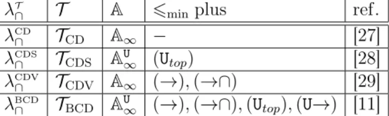
4. (Intersection type assignment systems λT
∩). We define in Figure 2.2 an infinite
collection of type assignment systems1 parametrized by a set of atoms A and a type
theory T . We name four particular type assignment systems in the table below, which is an excerpt from Figure 13.4 of [12]. Γ `T∩ M : σ denotes a derivable
type assignment judgment in the type assignment system λT
∩. Type checking is not
decidable for λCD
∩ , λCDV∩ , λCDS∩ , and λBCD∩ (see Theorem 2.24).
2.1.1
The ∆-calculi
Intersection type assignment systems and ∆-calculi have in common their type syntax and intersection type theories. The syntax of the generic ∆-calculus is defined as follows: Definition 2.2 (Generic ∆-calculus syntax).
∆ ::= uM | x | λx:σ.∆ | ∆ ∆ | h∆, ∆i | pri∆ | ∆σ i ∈ {1, 2}
Intuitively, uM denotes an infinite set of constants, indexed with a particular pure λ-term.
∆τ denotes an explicit coercion2 of a term ∆ to type τ , where the typing rules will ensure
that ∆ has a type σ such that σ 6T τ . The expression h∆, ∆i denotes a pair that,
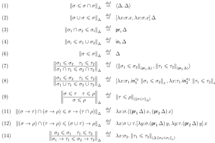
following the López-Escobar jargon [67], we call strong pair with respective projections pr1 and pr2. The essence function o _ o is an erasing function mapping typed ∆-terms into pure λ-terms. It is defined as follows:
Definition 2.3 (Essence function).
o x o def= x o ∆σo def= o ∆ o o u Mo def = M o λx:σ.∆ o def= λx.o ∆ o o ∆1∆2o def = o ∆1o o ∆2o o h∆1, ∆2i o def = o ∆1o o pri∆ o def = o ∆ o i ∈ {1, 2}
1Although rules (∩E
i) are derivable with 6min, we add them for clarity. 2If type coercions are implicit, then we lose the uniqueness of type property.
One could argue that the choice of o h∆1, ∆2i o def
= o ∆1o is arbitrary and could have
been replaced with o h∆1, ∆2i o def
= o ∆2o. However, the typing rules will ensure that, if
h∆1, ∆2i is typable, then, for some suitable equivalence relation R, we have that o ∆1o R
o ∆2o. Thus, strong pairs can be viewed as constrained cartesian products. The reduction
semantics reduces terms of the generic ∆-calculus as follows:
Definition 2.4 (Generic reduction semantics). Let syntactical equality by denoted by ≡. 1. (Substitution) Substitution on ∆-terms is defined as usual, with the additional
rules: uM[∆/x] def = u(M [o ∆ o/x]) ∆σ 1[∆2/x] def = (∆1[∆2/x])σ
2. (One-step reduction). We define three notions of reduction:
(λx:σ.∆1) ∆2 7→ ∆1[∆2/x] (β)
prih∆1, ∆2i 7→ ∆i i ∈ {1, 2} (pri)
λx:σ.∆ x 7→ ∆ x 6∈ Fv(∆) (η)
Observe that (λx:σ.∆1)σ∆2 is not a redex, because the λ-abstraction is coerced.
The contextual closure is defined as usual except for reductions inside the index of uM that are forbidden (even though substitutions are propagated). We write
−→βpri for the contextual closure of the (β) and (pri) notions of reduction, −→η
for the contextual closure of (η). We also define a synchronous contextual closure, which is like the usual contextual closure except for the strong pairs, as defined in point (3). Synchronous contextual closure of the notions of reduction generates the reduction relations −→kβpr
i and −→
k η.
3. (Synchronous closure of −→k). Synchronous closure is defined on the strong pairs with the following constraint:
∆1 −→k ∆01 ∆2 −→k ∆02 o ∆01o ≡ o∆02o
h∆1, ∆2i −→k h∆01, ∆ 0 2i
(Closk)
Note that we reduce in the two components of the strong pair. A longer and more detailed definition of synchronous reduction is given in Subsection 2.1.2;
4. (Multistep reduction). We write −→−→βpri (resp. −→−→
k
βpri) as the reflexive and
transitive closure of −→βpri (resp. −→ k βpri);
5. (Congruence). We write =βpri as the symmetric, reflexive, transitive closure of
−→−→βpri.
We mostly consider βpri-reductions, thus to ease the notation, we will often omit the subscript in βpri-reductions.
The next definition introduces a notion of synchronization inside strong pairs.
Definition 2.5 (Synchronization). A ∆-term is synchronous if and only if, for all its subterms of the shape h∆1, ∆2i, we have that o ∆1o ≡ o ∆2o.
Γ `TR ∆ : σ σ 6T τ Γ `TR ∆τ : τ (6T) Γ, x:σ `TR∆ : τ Γ `TRλx:σ.∆ : σ → τ (→I) Γ `TR∆1 : σ → τ Γ `TR ∆2 : σ Γ `TR∆1∆2 : τ (→E) x:σ ∈ Γ Γ `TRx : σ (ax) Γ `TR ∆1 : σ Γ `RT ∆2 : τ o ∆1o R o ∆2o Γ `TR h∆1, ∆2i : σ ∩ τ (∩I) U ∈ A Γ `TRuM : U (top) Γ `TR∆ : σ ∩ τ Γ `TRpr2∆ : τ (∩E2) Γ `TR∆ : σ ∩ τ Γ `TR pr1∆ : σ (∩E1) Figure 2.4: Generic ∆-calculus ∆T
R
It is easy to verify that −→k preserves synchronization, while it is not the case for −→. The next definition introduces an intersection typed system for the generic ∆-calculus that is parametrizable by R, a suitable equivalence relation on pure λ-terms, and T , a type theory, as follows:
Definition 2.6 (Generic ∆-calculus ∆T
R). The generic ∆-calculus is defined in Figure
2.4. We denote by ∆T
R a particular typed system with the type theory T and under an
equivalence relation R and by Γ `TR∆ : σ a corresponding typing judgment.
The typing rules are intuitive for a calculus à la Church except rules (∩I), (top) and (6T).
The typing rule for a strong pair (∩I) is similar to the typing rule for a cartesian product, except for the side-condition o ∆1o R o ∆2o, forcing the two parts of the strong
pair to have essences equivalent under R, thus making a strong pair a special case of a cartesian pair. For instance, hλx:σ.λy:τ.x, λx:σ.xi is not typable in ∆T
≡; meanwhile
h(λx:σ.x) y, yi is not typable in ∆T
≡ but it is in ∆ T
=β; and hx, λy:σ.(λz:τ.z) x yi is not
typable in ∆T
≡ nor ∆
T
=β but it is in ∆ T
=βη. In the typing rule (top), the subscript M in uM
is an arbitrary pure λ-term. The typing rule (6T) allows to change the type of a ∆-term
from σ to τ if σ 6T τ : the term in the conclusion must record this change with an explicit
type coercion _τ, producing the new term ∆τ: explicit type coercions are important to
keep the unicity of typing derivations.
The next definition introduces the generic intersection typed system. Definition 2.7 (Generic intersection typed system λ@T
R). For historical reasons (see
[63, 64, 40]), we used judgments where ∆-terms were decorated by their essence. We thus get judgments of the form Γ `TRM @∆ : σ for a system called λ@T
R. The derivation rules
are given in Figure 2.5. The properties of λ@T
R are the same than those of ∆ T
R, because
the decorations do nothing but make the terms easier to understand for newcomers. The next definition introduces a partial order over equivalence relations on pure λ-terms and an inclusion over typed systems as follows:
Γ `TRM @∆ : σ σ 6T τ Γ `TRM @∆τ : τ (6T) Γ, x:σ `TRM @∆ : τ Γ `TR λx.M @λx:σ.∆ : σ → τ (→I) Γ `TRM @∆1 : σ → τ Γ `TR N @∆2 : σ Γ `TR M N @∆1∆2 : τ (→E) x:σ ∈ Γ Γ `TR x@x : σ (ax) Γ `TRM @∆1 : σ Γ `TR N @∆2 : τ M R N Γ `TR M @h∆1, ∆2i : σ ∩ τ (∩I) U ∈ A Γ `TR M @uM : U (top) Γ `TRM @∆ : σ ∩ τ Γ `TRM @pr2∆ : τ (∩E2) Γ `TR M @∆ : σ ∩ τ Γ `TRM @pr1∆ : σ (∩E1)
Figure 2.5: Generic intersection typed system λ@T R
Definition 2.8 (R and v).
1. Let R ∈ {≡, =β, =βη}. R1 v R2 if, for all pure λ-terms M, N such that M R1 N ,
we have that M R2 N ;
2. ∆T1R1 v ∆T2
R2 if, for any Γ, ∆, σ such that Γ `
T1
R1 ∆ : σ, we have that Γ `
T2
R2 ∆ : σ.
Note that v correspond to the standard inclusion between relation. Proposition 2.1. 1. ∆CD R v ∆CDSR v ∆BCDR and ∆CDR v ∆CDVR v ∆BCDR ; 2. ∆T1R1 v ∆T2 R2 if T1 v T2 and R1 v R2.
2.1.2
The ∆-chair
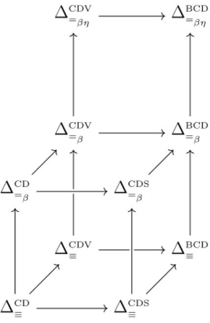
The next definition classifies ten instances of the generic ∆-calculus. Definition 2.9 (∆-chair). Ten typed systems ∆T
R can be draw in a diagram called
∆-chair, as in Figure 2.6, where the arrows represent an inclusion relation. ∆CD
≡ corresponds
roughly to [63, 64] (in the expression M @∆, M is the essence of ∆) and in its intersection part to [88]; ∆CDS
≡ corresponds roughly in its intersection part to [40], ∆ BCD
≡ corresponds
in its intersection part to [65], ∆CD
=βη corresponds in its intersection part to [39]. The other
typed systems are basically new. The main properties of these systems are: 1. All the ∆T
≡ systems enjoys the synchronous subject reduction property, the other
systems also enjoy ordinary subject reduction (Theorem 2.11); 2. All the systems strongly normalize (Theorem 2.21);
3. All the systems correspond to the to original type assignment systems except ∆CD =β, ∆CDV =β , ∆ CDV =βη and ∆ BCD =βη (Theorem 2.22);
4. Type checking and type reconstruction are decidable for all the systems, except ∆CDS =β , ∆ BCD =β , and ∆ BCD =βη (Theorem 2.24).
∆CD ≡ ∆CD =β ∆CDV ≡ ∆CDV =β ∆CDS ≡ ∆CDS =β ∆BCD ≡ ∆BCD =β ∆CDV =βη ∆ BCD =βη
Figure 2.6: The ∆-chair
2.2
Examples
This section shows examples of typed derivations ∆T
R and highlights the corresponding
type assignment judgment in λT
∩ they correspond to, in the sense that we have a derivation
Γ `TR ∆ : σ and another derivation Γ `T∩ o ∆ o : σ. The correspondence between intersec-tion typed systems ∆T
R and intersection type assignment λ T
∩ will be defined in Subsection
2.4.1.
Example 2.1 (Polymorphic identity). In all of the intersection type assignment systems λT
∩ we can derive:
`T∩ λx.x : (σ → σ) ∩ (τ → τ ) A corresponding ∆-term is:
hλx:σ.x, λx:τ.xi
It can be typed in all of the typed systems of the ∆-chair as follows: x:σ `TRx : σ `T Rλx:σ.x : σ → σ x:τ `TR x : τ `T R λx:τ.x : τ → τ λx.x R λx.x `T R hλx:σ.x, λx:τ.xi : (σ → σ) ∩ (τ → τ )
Example 2.2 (Auto application). In all of the intersection type assignment systems we can derive:
`T
∩ λx.x x : ((σ → τ ) ∩ σ) → τ
A corresponding ∆-term is:
λx:(σ → τ ) ∩ σ.(pr1x)(pr2x)
It can be typed in all of the typed systems of the ∆-chair as follows: x:(σ → τ ) ∩ σ `TR x : (σ → τ ) ∩ σ x:(σ → τ ) ∩ σ `TRpr1x : σ → τ x:(σ → τ ) ∩ σ `TR x : (σ → τ ) ∩ σ x:(σ → τ ) ∩ σ `TRpr2x : σ x:(σ → τ ) ∩ σ `TR(pr1x)(pr2x) : τ `T Rλx:(σ → τ ) ∩ σ.(pr1x)(pr2x) : (σ → τ ) ∩ σ → τ
Example 2.3 (Some examples in ∆CDS R ). In λ CDS ∩ we can derive: `TCDS ∩ (λx.λy.x) : σ → U → σ
Using this type assignment, we can derive: z:σ `TCDS
∩ (λx.λy.x) z z : σ
A corresponding ∆-term is:
(λx:σ.λy:U.x) z zU It can be typed in ∆CDS R as follows: z:σ, x:σ, y:U `TCDS R x : σ z:σ, x:σ `TCDS R λy:U.x : U → σ z:σ `TCDS R λx:σ.λy:U.x : σ → U → σ z:σ ` TCDS R z : σ z:σ `TCDS R (λx:σ.λy:U.x) z : U → σ z:σ `TCDS R z : σ σ 6TCDS U z:σ `TCDS R zU : U z:σ `TCDS R (λx:σ.λy:U.x) z zU : σ
As another example, we can also derive: `TCDS
∩ λx.x : σ → σ ∩ U
A corresponding ∆-term is:
λx:σ.hx, xUi It can be typed in ∆CDS R as follows: x:σ `TCDS R x : σ x:σ `TCDS R x : σ σ 6TCDS U x:σ `TCDS R xU : U x R x x:σ `TCDS R hx, xUi : σ ∩ U `TCDS R λx:σ.hx, xUi : σ → σ ∩ U
Example 2.4 (An example in ∆CDV
R ). In λ CDV
∩ we can prove the commutativity of
inter-section:
`TCDV
∩ λx.x : σ ∩ τ → τ ∩ σ
A corresponding ∆-term is:
hλx:σ ∩ τ.pr2x, λx:σ ∩ τ.pr1xi(σ∩τ )→(τ ∩σ) It can be typed in ∆CDV R as follows: x:σ ∩ τ `TCDS R x : σ ∩ τ x:σ ∩ τ `TCDS R pr2x : τ `TCDS R λx:σ ∩ τ.pr2x : (σ ∩ τ ) → τ x:σ ∩ τ `TCDS R x : σ ∩ τ x:σ ∩ τ `TCDS R pr1x : σ `TCDS R λx:σ ∩ τ.pr1x : (σ ∩ τ ) → σ λx.x R λx.x `TCDS R hλx:σ ∩ τ.pr2x, λx:σ ∩ τ.pr1xi : ((σ ∩ τ ) → τ ) ∩ ((σ ∩ τ ) → σ) ∗ `TCDS R hλx:σ ∩ τ.pr2x, λx:σ ∩ τ.pr1xi(σ∩τ )→(τ ∩σ) : (σ ∩ τ ) → (τ ∩ σ) where ∗ is ((σ ∩ τ ) → τ ) ∩ ((σ ∩ τ ) → σ)6TCDV (σ ∩ τ ) → (τ ∩ σ).
Example 2.5 (Another polymorphic identity in ∆T
=β). In all the ∆ T
=β you can type this
∆-term:
hλx:σ.x, (λx:τ →τ.x) (λx:τ.x)i The typing derivation is the following:
x:σ `T= β x : σ `T =β λx:σ.x : σ → σ x:τ → τ `T= β x : τ → τ `T =β λx:τ →τ.x : (τ → τ ) → (τ → τ ) x:τ `T= β x : τ `T =β λx:τ.x : τ → τ `T =β (λx:τ →τ.x) (λx:τ.x) : τ → τ λx.x =β (λx.x) (λx.x) `T =β hλx:σ.x, (λx:τ →τ.x) (λx:τ.x)i : (σ → σ) ∩ (τ → τ )
Example 2.6 (Two examples in ∆BCD
≡ and ∆
BCD
=βη). In λ BCD
∩ we can can type any term,
including the following non-terminating term:
Ωdef= (λx.x x) (λx.x x) More precisely, we have:
`TBCD
∩ Ω : U
A corresponding ∆-term whose essence is Ω is:
(λx:U.xU→Ux) (λx:U.xU→Ux)U
It can be typed in ∆BCD R as follows: ∗ `TBCD R λx:U.xU→Ux : U → U ∗ `TBCD R λx:U.xU→Ux : U → U U → U6TBCD U `TBCD R (λx:U.xU→Ux)U : U `TBCD
R (λx:U.xU→Ux) (λx:U.xU→Ux)U : U
where ∗ is: x:U `TBCD R x : U U6TBCD U → U x:U `TBCD R xU→U : U → U x:U ` TBCD R x : U x:U `TBCD R xU→Ux : U In λBCD
∩ we can type the following:
x:U → U `TBCD
∩ x : (U → U) ∩ (σ → U)
A corresponding ∆-term (whose essence is x) is: hx, λy:σ.x yUi It can be typed in ∆BCD =βη as follows: x:U → U `TBCD =βη x : U → U x:U → U, y:σ `TBCD =βη x : U → U x:U → U, y:σ `TBCD =βη y : σ σ 6 U x:U → U, y:σ `TBCD =βη y U : U x:U → U, y:σ `TBCD =βη x y U : U x:U → U `TBCD =βη λy:σ.x y U : σ → U x = βη λy.x y x:U → U `TBCD =βη hx, λy:σ.x y Ui : (U → U) ∩ (σ → U)
Note that the =βη condition has an interesting loophole, as it is well-known that λBCD∩
does not enjoy =η-conversion property. Theorem 2.17(1) will show that we can construct
a ∆-term which does not correspond to any λBCD
Example 2.7 (Pottinger [80]). The following examples can be typed in all the type theories of the ∆-chair (we also display in square brackets the corresponding pure λ-terms typable in λT
∩). These are encodings from the examples à la Curry given by Pottinger in
[80]. [λx.λy.x y] `T R λx:(σ → τ ) ∩ (σ → ρ).λy:σ.h(pr1x) y), (pr2x) yi : (σ → τ ) ∩ (σ → ρ) → σ → τ ∩ ρ [λx.λy.x y] `T
R λx:σ → τ ∩ ρ.hλy:σ.pr1(x y), λy:σ.pr2(x y)i : (σ → τ ∩ ρ) → (σ → τ ) ∩ (σ → ρ)
[λx.λy.x y] `T R λx:σ → ρ.λy:σ ∩ τ.x (pr1y) : (σ → ρ) → σ ∩ τ → ρ [λx.λy.x] `T R λx:σ ∩ τ.λy:σ.pr2x : σ ∩ τ → σ → τ [λx.λy.x y y] `T R λx:σ → τ → ρ.λy:σ ∩ τ.x (pr1y) (pr2y) : (σ → τ → ρ) → σ ∩ τ → ρ [λx.x] `TR λx:σ ∩ τ.pr1x : σ ∩ τ → σ [λx.x] `T R λx:σ.hx, xi : σ → σ ∩ σ [λx.x] `T R λx:σ ∩ (τ ∩ ρ).hhpr1x, pr1pr2xi, pr2pr2xi : σ ∩ (τ ∩ ρ) → (σ ∩ τ ) ∩ ρ
In the same paper, Pottinger lists some types that cannot be inhabited by any inter-section type assignment (6 `T∩) in an empty context, namely: σ → (σ ∩ τ ) and (σ → τ ) → (σ → ρ) → σ → τ ∩ ρ and ((σ ∩ τ ) → ρ) → σ → τ → ρ. It is not difficult to verify that the above types cannot be inhabited by any of the type systems of the ∆-chair because of the failure of the essence condition in the strong pair type rule.
Example 2.8 (Intersection is not the conjunction operator [55, 13]). This counter-example is from the corresponding counter-counter-example à la Curry given by Hindley [55] and Ben-Yelles [13]. The intersection type (σ → σ) ∩ ((σ → τ → ρ) → (σ → τ ) → σ → ρ) where the left part of the intersection corresponds to the type for the combinator I and the right part for the combinator S cannot be assigned to a pure λ-term. Analogously, the same intersection type cannot be assigned to any ∆-term belonging to a type system from the ∆-chair, because of the failure of the essence condition.
2.2.1
On synchronization and subject reduction
For the typed systems ∆T
≡, strong pairs have an intrinsic notion of synchronization: some
∆-terms that cannot be typed. Consider the ∆-term h(λx:σ.x) y, (λx:σ.x) yi. If we use the −→ reduction relation, then the following reduction paths are legal:
h(λx:σ.x) y, (λx:σ.x) yi 1
β h(λx:σ.x) y, yi
%β %β hy, (λx:σ.x) yi 1
β hy, yi
More precisely, the first and second redexes are rewritten asynchronously, therefore they cannot be typed in any typed system ∆T
≡, because we fail to check that the left and
the right part of the strong pair are syntactically the same: the −→k reduction relation prevents this loophole and allows to type all redexes. In summary, −→k can be thought of as the natural reduction relation for the typed systems ∆T
≡.
2.3
Metatheory of
∆
TR
2.3.1
General properties
Unless specified, all properties applies to the intersection typed systems ∆T R.
The Church-Rosser property is proved using the technique of Takahashi [90]. The parallel reduction semantics extends Definition 2.4 and it is inductively defined as follows: Definition 2.10 (Parallel reduction semantics).
x =⇒ x uM =⇒ uM ∆σ =⇒ (∆0)σ if ∆ =⇒ ∆0 ∆1∆2 =⇒ ∆01∆20 if ∆1 =⇒ ∆01 and ∆2 =⇒ ∆02 λx:σ.∆ =⇒ λx:σ.∆0 if ∆ =⇒ ∆0 (λx:σ.∆1) ∆2 =⇒ ∆01[∆02/x] if ∆1 =⇒ ∆01 and ∆2 =⇒ ∆02 h∆1, ∆2i =⇒ h∆01, ∆ 0 2i if ∆1 =⇒ ∆01 and ∆2 =⇒ ∆02 pri∆ =⇒ pri∆0 if ∆ =⇒ ∆0 and i ∈ {1, 2} prih∆1, ∆2i =⇒ ∆0i if ∆i =⇒ ∆0i and i ∈ {1, 2}
Intuitively, ∆ =⇒ ∆0 means that ∆0 is obtained from ∆ by simultaneous arbitrary con-tractions of some βpri-redexes possibly overlapping each other. Church-Rosser can be achieved by proving a stronger statement, namely:
∆ =⇒ ∆0 implies ∆0 =⇒ ∆∗
where ∆∗ is a ∆-term determined by ∆ and independent from ∆0. The statement (2.3.1) is satisfied by the term ∆∗ which is obtained from ∆ by contracting all the redexes existing in ∆ simultaneously, as is shown in the following definition.
Definition 2.11 (The map _∗). x∗ def= x u∗M def= uM (∆σ)∗ def= (∆∗)σ h∆1, ∆2i∗ def = h∆∗ 1, ∆ ∗ 2i (λx:σ.∆)∗ def= λx:σ.∆∗ (∆1∆2)∗ def = ∆∗1∆∗2 if ∆1∆2 is not a β-redex ((λx:σ.∆1) ∆2)∗ def = ∆∗1[∆∗2/x]
(pri∆)∗ def= pri∆∗ if ∆ is not a strong pair (prih∆1, ∆2i)∗
def
= ∆∗i i ∈ {1, 2}
The next technical lemma will be useful in showing that Church-Rosser for −→−→ can be inherited from Church-Rosser for =⇒.
Lemma 2.2. 1. If ∆1 −→ ∆01, then ∆1 =⇒ ∆01; 2. if ∆1 =⇒ ∆01, then ∆1−→−→∆01; 3. if ∆1 =⇒ ∆01 and ∆2 =⇒ ∆02, then ∆1[∆2/x] =⇒ ∆01[∆02/x]; 4. ∆1 =⇒ ∆∗1. Proof.
1. Let C[·] be an applicative context, ∆ either a β-redex or a pri-redex, and ∆0 its contractum, such that ∆1 ≡ C[∆] and ∆01 ≡ C[∆
0]. We can check that ∆ =⇒ ∆0,
and, by induction on C[·], we conclude that ∆1 =⇒ ∆01;
2. 3. 4. By induction on the structure of ∆1.
We can now prove the Church-Rosser property for the parallel reduction: Lemma 2.3 (Confluence property for =⇒). If ∆ =⇒ ∆0, then ∆0 =⇒ ∆∗. Proof. By induction on the shape of ∆.
– if ∆ ≡ x, then ∆0 ≡ x =⇒ x ≡ ∆∗; – if ∆ ≡ uM, then ∆0 ≡ uM =⇒ uM ≡ ∆∗;
– if ∆ ≡ ∆σ1, then, for some ∆01, we have that ∆1 =⇒ ∆01 and ∆
0 ≡ (∆0
1)σ, therefore,
– if ∆ ≡ h∆1, ∆2i, then, for some ∆01 and ∆02, we have that ∆1 =⇒ ∆01, ∆2 =⇒ ∆02 and ∆0 ≡ h∆0 1, ∆ 0 2i. By induction hypothesis, ∆ 0 =⇒ h∆∗ 1, ∆ ∗ 2i ≡ ∆ ∗ ; – if ∆ ≡ λx:σ.∆1, then, for some ∆01, we have that ∆1 =⇒ ∆01 and ∆
0 ≡ λx:σ.∆0 1. By
induction hypothesis, λx:σ.∆01 =⇒ λx:σ.∆∗1 ≡ ∆∗;
– if ∆ ≡ ∆1∆2 and ∆ is not a β-redex, then, for some ∆01 and ∆02, we have that
∆1 =⇒ ∆01, ∆2 =⇒ ∆02 and ∆ 0 ≡ ∆0 1∆ 0 2. By induction hypothesis, ∆ 0 =⇒ ∆∗ 1∆ ∗ 2 ≡ ∆∗;
– if ∆ ≡ (λx:σ.∆1) ∆2, then, for some ∆01 and ∆02, we have that ∆1 =⇒ ∆01, ∆2 =⇒ ∆02
and we have 2 subcases: – ∆0 ≡ (λx:σ.∆0 1) ∆ 0 2: by induction hypothesis, ∆ 0 =⇒ ∆∗ 1[∆ ∗ 2/x] ≡ ∆ ∗; – ∆0 ≡ ∆0 1[∆ 0 2/x]: we also have ∆ 0 =⇒ ∆∗ 1[∆ ∗
2/x], thanks to point (3) of Lemma
2.2;
– if ∆ ≡ pri∆1and ∆1 is not a strong pair, then, for some ∆01, we have that ∆1 =⇒ ∆01
and ∆0 ≡ pri∆01, therefore, by induction hypothesis, ∆0 =⇒ pri∆∗1 ≡ ∆∗;
– if ∆ ≡ prih∆1, ∆2i, then, for some ∆01 and ∆ 0
2, we have that ∆1 =⇒ ∆01, ∆2 =⇒ ∆02
and we have 2 subcases: – ∆0 ≡ prih∆0
1, ∆02i: by induction hypothesis, ∆0 =⇒ ∆∗i ≡ ∆∗;
– ∆0 ≡ ∆0
i: we also have, by induction hypothesis, ∆
0 =⇒ ∆∗ i ≡ ∆
∗.
The Church-Rosser property follows from Lemma 2.3. Theorem 2.4 (Confluence).
If ∆1−→−→∆2 and ∆1−→−→∆3, then there exists ∆4 such that ∆2−→−→∆4 and ∆3−→−→∆4.
Proof. Thanks to the first two points of Lemma 2.2, we know that −→−→ is the transitive closure of =⇒, therefore we can deduce the confluence property of −→−→ with the usual diagram chase, as suggested below.
∆0,0 ∆0,1 ∆0,2 ∆1,0 ∆1,1 ∆1,2 ∆2,0 ∆2,1 ∆2,2 ∆3,0 ∆3,1 ∆3,2
The next lemma says that all type derivations for ∆ have an unique type. Lemma 2.5 (Unicity of typing).
If Γ `TR∆ : σ, then σ is unique.
The next lemma proves inversion properties on typable ∆-terms. Lemma 2.6 (Inversion).
1. If Γ `TRx : σ, then x:σ ∈ Γ;
2. if Γ `TR λx:σ.∆ : ρ, then ρ ≡ σ → τ for some τ and Γ, x:σ `TR ∆ : τ ;
3. if Γ `TR ∆1∆2 : τ , then there is σ such that Γ `RT ∆1 : σ → τ and Γ `TR ∆2 : σ;
4. if Γ `TR h∆1, ∆2i : ρ, then there is σ, τ such that ρ ≡ σ ∩ τ and Γ `TR ∆1 : σ and
Γ `TR ∆2 : τ and o ∆1o R o ∆2o;
5. if Γ `TR pr1∆ : σ, then there is τ such that Γ `TR ∆ : σ ∩ τ ; 6. if Γ `TR pr2∆ : τ , then there is σ such that Γ `TR ∆ : σ ∩ τ ; 7. if Γ `TR uM : σ, then σ ≡ U;
8. if Γ `TR ∆τ : ρ, then ρ ≡ τ and there is σ such that σ 6T τ and Γ `TR∆ : σ.
Proof. The typing rules are uniquely syntax-directed, therefore we can immediately con-clude.
The next lemma says that all subterms of a typable ∆-term are typable too. Lemma 2.7 (Subterms typability).
If Γ `TR∆ : σ, and ∆0 is a subterm of ∆, then there exists Γ0 and τ such that Γ0 ⊇ Γ and Γ0 `T
R ∆0 : τ .
Proof. By induction on the derivation of Γ `TR ∆ : σ. For instance, let’s consider the case where the applied rule is (→ I). The other cases are similar. If the last applied rule is (→ I), then ∆ ≡ λx:σ1.∆1 and σ ≡ σ1 → σ2 for some σ1, σ2, and ∆1. Moreover, ∆0 is a
subterm of ∆1, and:
Γ, x:σ1 ` ∆1 : σ2
By induction hypothesis, we know that there is an extension Γ0 of Γ, x:σ1 such that
Γ0 `T
R ∆0 : τ . As Γ0 is also an extension of Γ, we can conclude.
As expected, the weakening and strengthening properties on contexts are verified. Lemma 2.8 (Free-variable properties).
1. If Γ `TR∆ : σ, and Γ0 ⊇ Γ, then Γ0 `T
R ∆ : σ;
2. if Γ `TR ∆ : σ, then Fv(∆) ⊆ Dom(Γ);
3. if Γ `TR ∆ : σ, Γ0 ⊆ Γ and Fv(∆) ⊆ Dom(Γ0), then Γ0 `T
R ∆ : σ.
Proof. By induction on the derivation of Γ `TR∆ : σ.
The next lemma also says that essence is closed under substitution. Lemma 2.9 (Substitution).
2. If Γ, x:σ `TR ∆1 : τ and Γ `TR∆2 : σ, then Γ `TR ∆1[∆2/x] : τ .
Proof.
1. by induction on the shape of ∆1;
2. by induction on the derivation. As an illustration, we show the case when the last applied rule is (∩I). In this case, we know that:
Γ, x:σ `TR h∆1, ∆01i : τ ∩ τ 0
and Γ `TR∆2 : σ
By induction hypothesis, we have:
Γ `TR∆1[∆2/x] : τ and Γ `TR∆ 0
1[∆2/x] : τ0
Moreover, thanks to point (1), we can show that: o ∆1[∆2/x] o R o ∆01[∆2/x] o
As a consequence:
Γ `TR ∆1[∆2/x] : τ Γ `TR∆01[∆2/x] : τ0 o ∆1[∆2/x] o R o ∆01[∆2/x] o
Γ `TRh∆1, ∆01i[∆2/x] : τ ∩ τ0
(∩I)
In order to prove subject reduction, we need to prove that reducing ∆-terms preserve the side-condition o ∆1o R o ∆2o when typing the strong pair h∆1, ∆2i. We prove this in
the following lemma.
Lemma 2.10 (Essence reduction).
1. if Γ `T≡ ∆1 : σ and ∆1 −→ ∆2, then o ∆1o =β o ∆2o;
2. for R ∈ {=β, =βη}, if Γ `TR∆1 : σ and ∆1 −→ ∆2, then o ∆1o R o ∆2o;
3. if Γ `T=
βη ∆1 : σ and ∆1 −→η ∆2, then o ∆1o =η o ∆2o.
Proof. If ∆1 is a redex, then we have three cases:
– if ∆1 ≡ (λx:σ.∆01) ∆ 00
1 and ∆2 is ∆01[∆ 00
1/x], then, thanks to Lemma 2.9(1) we have
that o ∆2o ≡ o ∆01o[o ∆001o/x], therefore o ∆1o =β o ∆2o;
– if ∆1 ≡ prih∆01, ∆02i and ∆2 is ∆0i, we know that ∆1 is typable in ∆TR, and thanks
to Lemma 2.6(4), we have that o ∆01o R o ∆0
2o. As a consequence, o ∆1o R o ∆2o;
– if ∆1 ≡ λx:σ.∆0x with x 6∈ Fv(∆0), and ∆2 is ∆0, then o ∆1o =η o ∆2o.
For the contextual closure, we have that ∆1 ≡ ∆[∆0/x], where ∆ acts as an applicative
context and ∆0 is a redex, and ∆2 is ∆[∆00/x] where ∆00 is the contractum of ∆0.
Then, as ∆0 is a subterm of ∆1, by Lemma 2.7 we deduce that ∆0 is typable, therefore
∆00 is also typable, and then we infer, using Lemma 2.9(1), that: o ∆1o ≡ o ∆ o[o ∆0o/x] and o ∆2o ≡ o ∆ o[o ∆00o/x]
![Figure 2.1: Minimal type theory 6 min , axioms and rule schemes (from Figure 13.2 and 13.3 of [12]) x:σ ∈ Γ Γ ` T ∩ x : σ (ax) Γ, x:σ ` T ∩ M : τΓ`T∩λx.M:σ → τ (→I) Γ ` T ∩ M : σ Γ ` T ∩ M : τ Γ ` T ∩ M : σ ∩ τ (∩I) Γ ` T ∩ M : σ → τ Γ ` T ∩ N : σΓ`T∩M N:τ](https://thumb-eu.123doks.com/thumbv2/123doknet/13038974.382282/25.892.187.715.478.707/figure-minimal-type-theory-axioms-rule-schemes-figure.webp)
![Figure 3.1: Intersection and union type assignment system λ BDdL [7]](https://thumb-eu.123doks.com/thumbv2/123doknet/13038974.382282/55.892.110.754.122.362/figure-intersection-union-type-assignment-λ-bddl.webp)
![Figure 3.2: Typed calculus λ@ BDdL [40]](https://thumb-eu.123doks.com/thumbv2/123doknet/13038974.382282/56.892.112.790.124.400/figure-typed-calculus-λ-bddl.webp)
![Figure 3.3 presents the main rules of ∆ BDdL of [39]: this system can be seen as a proof- proof-functional logic, in the sense of Pottinger [80] and López-Escobar [67]: formulæ encode, using the Curry-Howard isomorphism, derivations D : Γ ` M : σ in the ty](https://thumb-eu.123doks.com/thumbv2/123doknet/13038974.382282/57.892.145.750.126.390/figure-presents-functional-pottinger-escobar-formulæ-isomorphism-derivations.webp)
![Figure 6.2: The syntax of the ∆-framework Chapter 7 and Bull and Bull-Subtyping in [87]).](https://thumb-eu.123doks.com/thumbv2/123doknet/13038974.382282/95.892.242.645.116.623/figure-syntax-framework-chapter-bull-bull-subtyping.webp)