HAL Id: hal-02904945
https://hal.archives-ouvertes.fr/hal-02904945
Submitted on 24 Jul 2020HAL is a multi-disciplinary open access archive for the deposit and dissemination of sci-entific research documents, whether they are pub-lished or not. The documents may come from teaching and research institutions in France or abroad, or from public or private research centers.
L’archive ouverte pluridisciplinaire HAL, est destinée au dépôt et à la diffusion de documents scientifiques de niveau recherche, publiés ou non, émanant des établissements d’enseignement et de recherche français ou étrangers, des laboratoires publics ou privés.
An assessment of Earth’s climate sensitivity using
multiple lines of evidence
S. Sherwood, M. Webb, J. Annan, K. Armour, P. Forster, J. Hargreaves, G.
Hegerl, S. Klein, K. Marvel, E. Rohling, et al.
To cite this version:
S. Sherwood, M. Webb, J. Annan, K. Armour, P. Forster, et al.. An assessment of Earth’s climate sensitivity using multiple lines of evidence. Reviews of Geophysics, American Geophysical Union, 2020, �10.1029/2019RG000678�. �hal-02904945�
An assessment of Earth’s climate
sensitivity using multiple lines of
evidence
Authors: S. Sherwood
1, M.J. Webb
2, J.D. Annan
3, K.C. Armour
4, P.M. Forster
5, J.C.
Hargreaves
3, G. Hegerl
6, S. A. Klein
7, K.D. Marvel
8,20, E.J. Rohling
9,10, M.
Watanabe
11, T. Andrews
2, P. Braconnot
12, C.S. Bretherton
4, G.L. Foster
10, Z.
Hausfather
13, A.S. von der Heydt
14, R. Knutti
15, T. Mauritsen
16, J.R. Norris
17, C.
Proistosescu
18, M. Rugenstein
19, G.A. Schmidt
20, K.B. Tokarska
6,15, M.D. Zelinka
7.
Affiliations:
1. Climate Change Research Centre and ARC Centre of Excellence for Climate Extremes, UNSW Sydney, Sydney, Australia
2. Met Office Hadley Centre, Exeter, UK 3. Blue Skies Research Ltd, Settle, UK
4. School of Oceanography and Department of Atmospheric Sciences, University of Washington, Seattle, USA
5. Priestley International Centre for Climate, University of Leeds, UK 6. School of Geosciences, University of Edinburgh, UK
7. PCMDI, LLNL, California, USA
8. Dept. of Applied Physics and Applied Math, Columbia University, New York, NY, USA 9. Research School of Earth Sciences, Australian National University, Acton, ACT 2601,
Canberra, Australia
10. Ocean and Earth Science, University of Southampton, National Oceanography Centre, Southampton, UK
11. Atmosphere and Ocean Research Institute, The University of Tokyo, Japan
12. Laboratoire des Sciences du Climat et de l’Environnement, unité mixte CEA-CNRS-UVSQ, Université Paris-Saclay, Gif sur Yvette, France
13. Energy and Resources Group, UC Berkeley, USA
14. Institute for Marine and Atmospheric Research, and Centre for Complex Systems Science, Utrecht University, The Netherlands
15. Institute for Atmospheric and Climate Science, ETH Zurich, Switzerland 16. Department of Meteorology, Stockholm University, Sweden
17. Scripps Institution of Oceanography, UCSD, La Jolla CA, USA
18. Department of Atmospheric Sciences and Department of Geology, University of Illinois Urbana Champaign, IL, USA
19. Max Planck Institute for Meteorology, Hamburg, Germany 20. NASA Goddard Institute for Space Studies, New York, NY, USA
Key Points:
● We assess evidence relevant to Earth’s climate sensitivity S: feedback process understanding, and the historical and paleo-climate records.
● All three lines of evidence are difficult to reconcile with S < 2 K, while paleo evidence provides the strongest case against S > 4.5 K.
● A Bayesian calculation finds a 66% range of 2.6-3.9 K, which remains within the bounds 2.3-4.5 K under plausible robustness tests.
Corresponding Author Address: Steven Sherwood, Climate Change Research Centre,
UNSW Sydney, Kensington 2052 Australia.
Final version submitted to Rev. Geophysics and WCRP on 15th July 2020
Table of Contents:
Abstract 1. Introduction 2. Methods2.1. Measures of climate sensitivity 2.2. Physical Model
2.3. Statistical Method: Summary
2.4. Statistical Method: Further Information
2.4.1. Introduction to Bayesian Inference modelling 2.4.2. Description of methods and calculations
2.4.3. Specification of priors and novel aspects of our approach 2.4.4. Calculation of likelihoods and sampling method
3. Constraints from Process Understanding 3.1. Introductory concepts
3.1.1. Definitions of CO2 radiative forcing and climate feedbacks
3.1.2. Lines of evidence for process understanding 3.1.3. Methodology for assessing process understanding 3.1.4. Further considerations
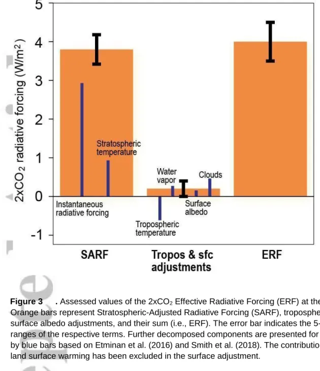
3.2. Process understanding of CO2 radiative forcing and non-cloud feedbacks
3.2.1. CO2 radiative forcing
3.2.2. Planck feedback
3.2.3. Water vapor and lapse rate feedbacks 3.2.4. Surface albedo feedback
3.2.5. Stratospheric feedback
3.2.6. Feedbacks from other atmospheric composition changes 3.3. Process understanding of cloud feedbacks
3.3.1. High cloud altitude feedback
3.3.2. Tropical marine low cloud feedback 3.3.3. Tropical anvil cloud area feedback 3.3.4. Land cloud feedback
3.3.5. Mid-latitude marine low-cloud amount feedback 3.3.6. High-latitude low-cloud optical depth feedback 3.4. Process assessment of λ and implications for S
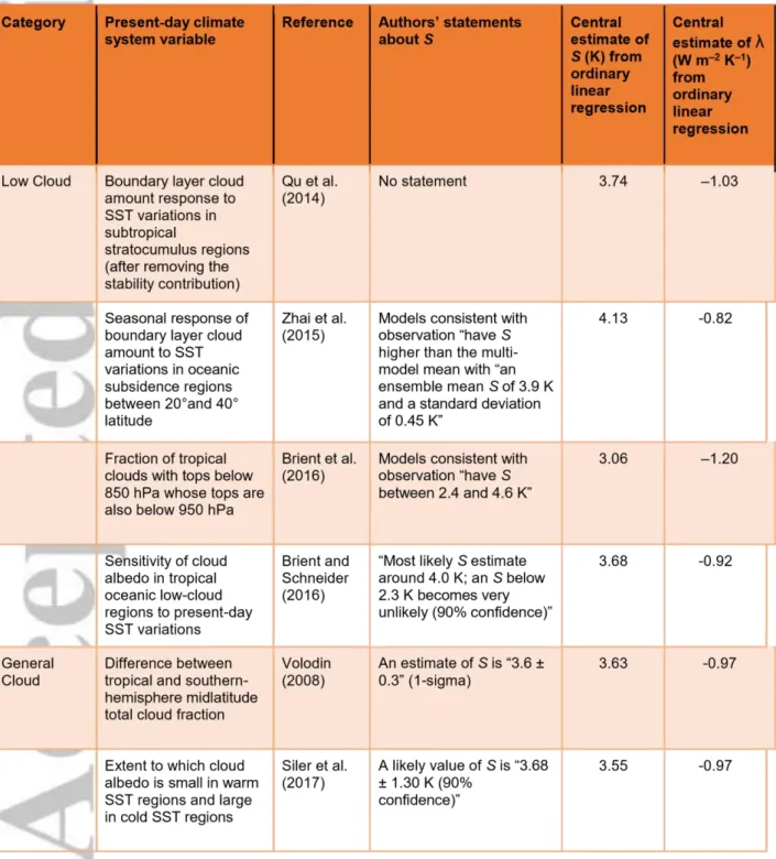
3.5. Constraints from observations of global inter-annual radiation variability 3.6. Emergent constraints on S from present-day climate system variables 3.7. Summary
4. Constraints from the Historical Climate Record 4.1. Inferring Shist from the historical climate record
4.1.1. Observationally based estimates, their inputs and uncertainties 4.1.2. Computing the likelihood
4.1.3. Consistency with estimates based on other forward models 4.1.4. Why is Shist uncertain?
4.2. Transitioning from Shist to S
4.2.1. Quantifying the historical pattern effect 4.3. Summary
5. Constraints from Paleoclimate Records
5.1. Methodology for estimating sensitivity from paleoclimate information 5.1.1. Energy balance approach
5.1.2. Estimating climates in the past—methods and sources of uncertainty 5.2. Evidence from cold periods: LGM and glacial-interglacial transitions
5.2.1. Surface temperature change ∆T 5.2.2. Forcings contributing to ∆F
5.2.3. Corrections for state-dependence of sensitivity and slowness of equilibration 5.2.4. Discussion
5.3. Evidence from warm periods 5.3.1. Mid-Pliocene
5.3.2. Paleocene-Eocene Thermal Maximum 5.4. Combining constraints from warm and cold periods 5.5. Summary
6. Dependence Between Lines of Evidence 6.1. Use of GCMs
6.2. Potential co-dependencies 6.3. Simple dependence test 6.4. Summary
7. Quantitative Synthesis of Evidence for S 7.1. Baseline calculation
7.2. Sensitivity to choice of prior
7.3. Sensitivity to specification of evidence
7.4. Implications for related sensitivity measures and future warming 7.5. Limitations, caveats and potential future approaches
7.6. Summary
8. Summary and Conclusions 8.1. Considerations 8.2. Key findings
8.3. Caveats and look forward
9. Acknowledgements and author contributions.
10. References
Abstract
We assess evidence relevant to Earth’s equilibrium climate sensitivity per doubling of
atmospheric CO
2, characterized by an effective sensitivity S. This evidence includes
feedback process understanding, the historical climate record, and the paleoclimate
record. An S value lower than 2 K is difficult to reconcile with any of the three lines of
evidence. The amount of cooling during the Last Glacial Maximum provides strong
evidence against values of S greater than 4.5 K. Other lines of evidence in
combination also show that this is relatively unlikely. We use a Bayesian approach to
produce a probability density (PDF) for S given all the evidence, including tests of
robustness to difficult-to-quantify uncertainties and different priors. The 66% range is
2.6-3.9 K for our Baseline calculation, and remains within 2.3-4.5 K under the
robustness tests; corresponding 5-95% ranges are 2.3-4.7 K, bounded by 2.0-5.7 K
(although such high -confidence ranges should be regarded more cautiously). This
indicates a stronger constraint on S than reported in past assessments, by lifting the
low end of the range. This narrowing occurs because the three lines of evidence
agree and are judged to be largely independent, and because of greater confidence
in understanding feedback processes and in combining evidence. We identify
promising avenues for further narrowing the range in S, in particular using
comprehensive models and process understanding to address limitations in the
traditional forcing-feedback paradigm for interpreting past changes.
Plain Language Summary
Earth’s global “climate sensitivity” is a fundamental quantitative measure of the susceptibility of Earth’s climate to human influence. A landmark report in 1979 concluded that it probably lies between 1.5-4.5℃ per doubling of atmospheric carbon dioxide, assuming that other influences on climate remain unchanged. In the 40 years since, it has appeared difficult to reduce this uncertainty range. In this report we thoroughly assess all lines of evidence including some new developments. We find that a large volume of consistent evidence now points to a more confident view of a climate sensitivity near the middle or upper part of this range. In particular, it now appears extremely unlikely that the climate sensitivity could be low enough to avoid substantial climate change (well in excess of 2℃ warming) under a high-emissions future scenario. We remain unable to rule out that the sensitivity could be above 4.5℃ per doubling of carbon dioxide levels, although this is not likely. Continued research is needed to further reduce the uncertainty and we identify some of the more promising possibilities in this regard.
1 Introduction
Earth’s equilibrium climate sensitivity (ECS), defined generally as the steady-state global temperature increase for a doubling of CO2, has long been taken as the starting point for
understanding global climate changes. It was quantified specifically by Charney et al. (National Research Council, 1979) as the equilibrium warming as seen in a model with ice sheets and vegetation fixed at present-day values. Those authors proposed a range of
1.54.5 K based on the information at the time, but did not attempt to quantify the probability that the sensitivity was inside or outside this range. The most recent report by the
Intergovernmental Panel on Climate Change (Stocker et al., 2013) asserted the same nowfamiliar range, but more precisely dubbed it a >66% (“likely”) credible interval, implying an up to one in three chance of being outside that range. It has been estimated that—in an ideal world where the information would lead to optimal policy responses—halving the uncertainty in a measure of climate sensitivity would lead to an average savings of US$10 trillion in today’s dollars (Hope, 2015). Apart from this, the sensitivity of the world’s climate to external influence is a key piece of knowledge that humanity should have at its fingertips. So how can we narrow this range?
Quantifying ECS is challenging because the available evidence consists of diverse strands, none of which is conclusive by itself. This requires that the strands be combined in some way. Yet, because the underlying science spans many disciplines within the Earth Sciences, individual scientists generally only fully understand one or a few of the strands. Moreover, the interpretation of each strand requires structural assumptions that cannot be proven, and sometimes ECS measures have been estimated from each strand that are not fully
equivalent. This complexity and uncertainty thwarts rigorous, definitive calculations and gives expert judgment and assumptions a potentially large role.
Our assessment was undertaken under the auspices of the World Climate Research Programme's Grand Science Challenge on Clouds, Circulation and Climate Sensitivity following a 2015 workshop at Ringberg Castle in Germany. It tackles the above
issues, addressing three questions:
1) Given all the information we now have, acknowledging and respecting the
uncertainties, how likely are very high or very low climate sensitivities, i.e., outside the presently accepted likely range of 1.5-4.5 K (IPCC, 2013)?
2) What is the strongest evidence against very high or very low values?
3) Where is there potential to reduce the uncertainty?
In addressing these questions, we broadly follow the example of Stevens et al. (2016,
hereafter SSBW16) who laid out a strategy for combining lines of evidence and transparently considering uncertainties. The lines of evidence we consider, as in SSBW16, are modern observations and models of system variability and feedback processes; the rate and trajectory of historical warming; and the paleoclimate record. The core of the combination strategy is to lay out all the circumstances that would have to hold for the climate sensitivity to be very low or high given all the evidence (which SSBW16 call “storylines”). A formal assessment enables quantitative probability statements given all evidence and a prior distribution, but the “storyline” approach allows readers to draw their own conclusions about how likely the storylines are, and points naturally to areas with greatest potential for further progress. Recognizing that expert judgment is unavoidable, we attempt to incorporate it in a transparent and consistent way (e.g., Oppenheimer et al., 2016).
Combining multiple lines of evidence will increase our confidence and tighten the range of likely ECS if the lines of evidence are broadly consistent. If uncertainty is underestimated in any individual line of evidence—inappropriately ruling out or discounting part of the ECS range—this will make an important difference to the final outcome (see example in Knutti et al., 2017). Therefore, it is vital to seek a comprehensive estimate of the uncertainty of each
line of evidence that accounts for the risk of unexpected errors or influences on the evidence. This must ultimately be done subjectively. We will therefore explore the
uncertainty via sensitivity tests and by considering ‘what if’ cases in the sense of SSBW16, including what happens if an entire line of evidence is dismissed.
The most recent reviews (Collins et al., 2013, Knutti et al., 2017) have considered the same three main lines of evidence considered here, and have noted they are broadly consistent with one another, but did not attempt a formal quantification of the PDF of ECS. Formal Bayesian quantifications have been done based on the historical warming record (see Bodman and Jones 2016 for a recent review), the paleoclimate record (PALAEOSENS, 2012), a combination of historical and last millennium records (Hegerl et al., 2006), and multiple lines of evidence from instrumental and paleo records (Annan and Hargreaves, 2006). An assessment based only on a subset of the evidence will yield too wide a range if the excluded evidence is consistent (e.g. Annan and Hargreaves, 2006), but if both subsets rely on similar information or assumptions, this co-dependence must be considered when combining them (Knutti and Hegerl 2008). Therefore, an important aspect of our assessment is to explicitly assess how uncertainties could affect more than one line of evidence (cf. section 6), and to assess the sensitivity of calculated PDFs to reasonable allowance for interdependencies of the evidence.
Another key aspect of our assessment is that we explicitly consider process understanding via modern observations and process models as a newly robust line of evidence (section 3). Such knowledge has occasionally been incorporated implicitly (via the prior on ECS) based on the sample distribution of ECS in available climate models (Annan and Hargreaves, 2006) or expert judgments (Forest et al., 2002), but climate models and expert judgments do not fully represent existing knowledge or uncertainty relevant to climate feedbacks, nor are they fully independent of other evidence (in particular that from the historical temperature record, see Kiehl, 2007). Process understanding has recently blossomed, however, to the point where substantial statements can be made without simply relying on climate model representations of feedback processes, creating a new opportunity exploited here.
Climate models (specifically general circulation models, or GCMs) nonetheless play an increasing role in calculating what our observational data would look like under various hypothetical ECS values—in effect translating from evidence to ECS. Their use in this role is now challenging long-held assumptions, for example showing that 20th-century warming could have been relatively weak even if ECS were high (section 4), that paleoclimate
changes are strongly affected by factors other than CO2, and that climate may become more
sensitive to greenhouse gases in warmer states (section 5). GCMs are also crucial for confirming how modern observations of feedback processes are related to ECS (section 3). Accordingly, another novel feature of this assessment will be to use GCMs to refine our expectations of what observations should accompany any given value of ECS and thereby avoid biases now evident in some estimates of ECS based on the historical record using simple energy budget or energy balance model arguments. GCMs are also used to link global feedback strengths to observable phenomena. However, for reasons noted above, we avoid relying on GCMs to tell us what values to expect for key feedbacks except where the feedback mechanisms can be calibrated against other evidence. Since we use GCMs in some way to help interpret all lines of evidence, we must be mindful that any errors in doing this could reinforce across lines (see section 6.2).
We emphasize that this assessment begins with the evidence on which previous studies were based, including new evidence not used previously, and aims to comprehensively synthesize the implications for climate sensitivity both by drawing on key literature and by doing new calculations. In doing this, we will identify structural uncertainties that have caused previous studies to report different ranges of ECS from (essentially) the same evidence, and account for this when assessing what that underlying evidence can tell us.
An issue with past studies is that different or vague definitions of ECS may have led to perceived, unphysical discrepancies in estimates of ECS that hampered abilities to constrain its range and progress understanding. Bringing all the evidence to bear in a consistent way requires using a specific measure of ECS, so that all lines of evidence are linked to the same underlying quantity. We denote this quantity S (see section 2.1). The implications for S of the three strands of evidence are examined separately in sections 3-5, and anticipated
dependencies between them are discussed in section 6. To obtain a quantitative PDF of S, we follow SSBW16 and many other studies by adopting a Bayesian formalism, which is outlined in sections 2.2-2.6. The results of applying this to the evidence are presented in section 7, along with the implications of our results for other measures of climate sensitivity and for future warming. The overall conclusions of our assessment are presented in section 8. We note that no single metric such as S can fully describe or predict climate responses, and we discuss its limitations in section 8.2, as well as implications of our work for future research.
While we endeavor to write for a broad audience, it is necessary to dip into technical detail in order to support the reasoning and conclusions, and some of the methods used are novel and require explanation. We have therefore structured this assessment so that the
discussions of the three lines of evidence (sections 3-5) are quasi-independent, with
separate introductions, detailed analyses, and conclusions. Readers who are not interested in the details can gain an overview of the key points from the concluding portions of these sections. Likewise, readers not interested in details of the statistical method could skip most of section 2 and focus on the “storylines” presented in sections 3-5. The probabilities given in section 7 derive from the statistical method, but the independence issues discussed in section 6 are important for either quantitative or qualitative assessment of the evidence.
2. Methods
This section first explains the measure of ECS we will use and how it relates to others (section 2.1), then presents the simple physical model used to interpret evidence (section 2.2). Section 2.3 summarizes the overall methodology, and section 2.4 goes over this in more detail, beginning with a basic review of Bayesian inference intended mainly for those new to the topic while focusing on concepts relevant to the ECS problem (section 2.4.1), then working through the solution of the model and sampling approach (sections 2.4.22.4.4). For other basic introductions to Bayesian inference, see Stone (2012) or Gelman et al. (2013).
2.1 Measures of climate sensitivity
Climate sensitivity is typically quantified as warming per doubling of CO2, but this is by
tradition. One could also consider the warming per unit radiative forcing, or the increment of additional net power exported to space per unit warming (the feedback parameter, i.e, energetic “spring constant” of the system) denoted λ. Indeed (see sections 2.2 and later) we will find it easier to write our evidence in terms of λ rather than warming-per-doubling (ECS), making the definition of an ECS optional. One can imagine a range of CO2 forcing scenarios,
each yielding its own value for the ECS; each such scenario also implies a matching value for λ. Our approach simultaneously constrains both λ and S (see section 2.3).
In choosing the reference scenario to define sensitivity for this assessment, for practical reasons we depart from the traditional Charney ECS definition (equilibrium response with ice sheets and vegetation assumed fixed) in favor of a comparable and widely used, so-called “effective climate sensitivity” S derived from system behavior during the first 150 years following a (hypothetical) sudden quadrupling of CO2. During this time the system is not in
equilibrium, but regression of global-mean top-of-atmosphere energy imbalance onto
globalmean near-surface air temperature, extrapolated to zero imbalance, yields an estimate of the long-term warming valid if the average feedbacks active during the first 150 years persisted to equilibrium (Gregory et al., 2004). This quantity therefore approximates the long-term Charney ECS (e.g., Danabasoglu and Gent, 2009), though how well it does so is a matter of active investigation addressed below. Our reference scenario does not formally exclude any feedback process, but the 150-year time frame minimizes slow feedbacks (especially ice sheet changes).
This choice involves weighing competing issues. Crucially, effective sensitivity (or other measures based on behavior within a century or two of applying the forcing) is more relevant to the time scales of greatest interest (i.e., the next century) than is equilibrium sensitivity, and effective sensitivity has been found to be strongly correlated (r=0.95) with the magnitude of model-simulated 21st-century warming under a high-emission scenario (Gregory et al., 2015, Grose et al., 2017, 2018). It is also widely available from climate models (e.g., Andrews et al., 2012) which facilitates many steps in our analysis. All candidate climate sensitivity measures are based on an outcome of a hypothetical scenario never realized on Earth. Ultimately models or theory are required to relate the outcome of any one scenario to that of any other. The ideal measure S is one that is as closely related as possible to
scenarios of practical interest: those which produced evidence (e.g., the historical CO2 rise),
or which might occur in the future. Effective sensitivity is a compromise that is relatively well related to both the available
past evidence and projected
future warmings
.
The Transient Climate Response (TCR, or warming at the time of CO2 doubling in an
idealized 1% per year increase scenario), has been proposed as a better measure of warming over the near- to medium-term; it may be more generally related to peak warming, and better constrained (in absolute terms) by historical warming, than S (Frame et al., 2005; Froelicher et al., 2013). It may also be better at predicting high-latitude warming (Grose et al., 2017). But as mentioned above, 21st-century global-mean trends under high emissions are better predicted by S than by TCR, perhaps because of nonlinearities in forcing or response (Gregory et al., 2015) or because TCR estimates are affected by noise
(Sanderson, 2020). TCR is also less directly related to the other lines of evidence than is S. In this study we will briefly address TCR in sections 4 and 7.4, but will not undertake a detailed assessment.
The IPCC (at least through AR5) formally retains a definition of ECS based on long-term equilibrium. Much of the information they use to quantify ECS however exploits GCM calculations of effective (e.g., Andrews et al., 2012), not equilibrium, sensitivity, and it appears that the distinction is often overlooked. In this report, we will use “long-term” to describe processes and responses involved in the effective sensitivity S, and “equilibrium” for the fully equilibrated ECS. The ECS differs from S due to responses involving the deep ocean, atmospheric composition and land surface that emerge on centennial time scales (e.g., Frey and Kay, 2018; see section 5), though calculations here (following Charney and past IPCC reports) do not include ice-sheet changes.
To calculate the ECS in a fully coupled climate model requires very long integrations (>1000 years). Fortunately, a recent intercomparison project (LongrunMIP; Rugenstein et al., 2019a) has organized long simulations from enough models to now give a reasonable idea of how ECS and S are likely to be related.
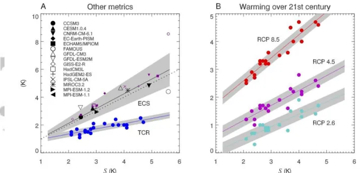
Relationships between S and several other quantities are shown in Fig. 1
from available models. Predicted S is reasonably well correlated with the other sensitivity measures (Fig. 1
a), indicating that S is a useful measure, but also that the conclusions of this assessment would still hold if another measure were used. Note that we do not consider here all possible measures; see Rugenstein et al. (2019b) for a discussion of some additional ones, which also generally correlate well with S. S is less well correlated to TCR (r=0.81) than to ECS (r=0.94), as expected since the TCR is sensitive to ocean heat uptake efficiency as well as to λ.
Although the measures correlate well, all available LongRunMIP models equilibrate to a higher warming at 4xCO2 than S from the same simulation (Fig. 1
a, small symbols;
details of how the equilibrium is estimated are given in Rugenstein et al. (2019a,b). The median equilibrium warming per doubling at 4xCO2 is 17% higher than the median S,
suggesting a robust amplifying impact of processes too slow to emerge in the first 150 years. This occurs due to responses of the climate system on multidecadal to millennial time
scales, including “pattern effects” from differences between ocean surface warming patterns that have not fully equilibrated within the first century or two (sections 3.3.2, 4.2); slow responses of vegetation; and temperature dependence of feedbacks. Evidence also shows, however (section 5.2.3), that sensitivity to two doublings (as assumed for S) is somewhat greater than that to one doubling. This state-dependence partly cancels out the low bias in the 150-year regression, leading to an ECS (for one doubling) that averages only 6% greater than S over the simulations, although the ratio of the two is uncertain so we assign an
uncertainty of ±20% (about 50%
wider than the sample standard deviation in the available GCMs). Thus, statements about S in this assessment can also be interpreted, to relatively good approximation, as statements about ECS for one doubling of CO2. (We use
the symbol ζ to represent this difference, with 1+ζ therefore being the ratio of our target S to the long-term equilibrium.)
Fig. 1
b shows the relationships of S to future warming. The warming trend over the 21st century (Fig. 1
b) is also well correlated with S, especially for the highest-emission scenario RCP8.5. The correlations are not quite as strong for the weaker-forcing cases, suggesting that global temperature changes are harder to predict (in a relative sense) in more highly mitigated scenarios. This is mostly due to a weaker warming signal, but there is also a slightly greater model spread, reasons for which are not currently understood.
To conclude, the effective sensitivity S that we will use—a linear approximation to the equilibrium warming based on the first 150 years after an abrupt CO2 quadrupling—is a
practical option for measuring sensitivity, based on climate system behavior over the most relevant time frame while still approximating the traditional ECS. Moreover, the quantitative difference between this and the traditional equilibrium measure based on a CO2 doubling
(with fixed ice sheets) appears to be small, albeit uncertain. This uncertainty is skewed, in the sense that long-term ECS could be substantially higher than S but is very unlikely to be substantially lower. Further work is needed to better understand and constrain this
uncertainty.
2.2 Physical model
Here we review the equations that will be used to relate the evidence to the key unknowns. According to the conventional forcing-feedback theory of the climate system, the net
downward radiation imbalance ∆N at the top-of-atmosphere (TOA) can be decomposed into a radiative forcing ∆F, a radiative response ∆R due directly or indirectly to forced changes in temperature which is the feedback, and variability V unrelated to the forcing or feedback:
∆𝑁 = ∆𝐹 + 𝛥𝑅 + 𝑉 (1
)
Variability V can arise due to unforced variations in upwelling of cold water to the surface, cloud cover, albedo, etc. The net radiation balance ∆N consists of the net absorbed shortwave (SW) solar radiation minus the planet’s emission of longwave (LW) radiation. Taking the radiative response ∆R as proportional to first order to the forced change in global mean surface air temperature ∆T, equation (1
) becomes
∆𝑁 = ∆𝐹 + 𝜆∆𝑇+ 𝑉 (
2) where the climate feedback parameter λ is defined as the sensitivity of the net TOA downward radiation N to T, dN/dt, (at fixed F). If this feedback parameter is negative, the system is stable.
In equilibrium over sufficiently long time-scales (assuming λ<0) the net radiation imbalance ∆N and mean unforced variability V will each be negligible, leaving a balance between the (constant) forcing ∆F and radiative response ∆R. In this case equation (
2) can be written
𝛥
𝑇 = −𝛥𝐹/𝜆 (3)
The case of a doubling of CO2 defines the climate sensitivity ∆𝐹2𝑥𝐶𝑂2
𝑆= − 𝜆 ,
(
4)
where ∆F2xCO2 is defined as the radiative forcing per CO2 doubling (noting that since our
reference scenario involves two doublings, ∆F2xCO2 is defined as half the effective forcing in
above equations assume equilibrium, our reference scenario (section 2.1) is not an
equilibrium scenario; however, because in this scenario ∆N is zero (by construction) at the time of the projected equilibrium warming ∆T, these equations still hold.
Finally we note that the total system feedback λ can be decomposed into the additive effect of multiple feedbacks in the system of strengths λi,
λ = Σ λi. (
5)
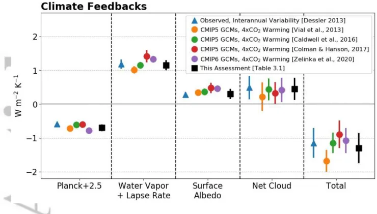
These feedbacks represent how the TOA radiation balance is altered as the climate warms by forced changes in identified radiatively active constituents of the climate system. In this study these are represented as six feedback components: the Planck feedback, combined water vapor and lapse rate feedback, total cloud feedback, surface albedo feedback, stratospheric feedback and an additional atmospheric composition feedback. These
individual feedback components are elaborated in section 3, where evidence is presented to constrain each of them (sections 3.3, 3.4; Table
1). Other process evidence is presented (section 3.5) which constrains the total, λ. Finally, so-called “emergent-constraint” studies are discussed (section 3.6) which tie S to some observable in the present-day climate, thereby constraining λ and S. For reasons discussed later however they are not used in our Baseline calculation, but are explored via a sensitivity test.
The other evidence used (sections 4, 5) comes from past climate changes and typically is interpreted via eq
s. (
2,
3) in previous climate sensitivity studies. These have typically assumed that the equations apply to any relevant climate change with universal values of λ and S, provided that the same feedbacks are counted therein (cf. eq
. (
5)). We will likewise apply these equations simultaneously to different past climate change scenarios, leading to a set of relationships shown graphically in Figure
2 (which offers a picture of our overall model, in particular its dependence structure; see section 2.4.2 for more information).
Recent work however has shown that effective λ (the value that satisfies eq. (
2) for some climate-change scenario) can vary significantly across scenarios even when the same feedbacks are nominally operating. All measurements relevant to climate sensitivity come from the recent historical period (during which internal variability may play a large role and the climate is far out of equilibrium; section 4) or from proxy reconstructions of past climate equilibria (during which the climate may have been quite different to that of the reference scenario; section 5). Thus, possible variations in the apparent λ during those time periods must be accounted for. Two particular issues are recognized. First, feedbacks can change strength in different climate states due to direct dependence on global temperature or indirect dependence (e.g. via snow or ice cover), or other differences in the earth system (e.g., topography). Second, the net outgoing radiation ∆N can depend not only on the global mean surface temperature but also on its geographic pattern ∆T’, leading to an apparent dependence of λ on ∆T’ when applying eq. (
2). Such pattern variations can arise either because of heterogeneous radiative forcings, lag-dependent responses to forcings, or unforced variability. To use such observations to constrain our S and λ, it is important to account for these effects. Note that these effects are distinct from atmospheric “adjustments” to applied radiative forcings (Sherwood et al., 2015), which scale with the forcing and are included as part of the effective radiative forcing ∆F.
We account for impacts on λ by defining an additive correction ∆λ for each past climate change
representing the difference between its apparent λ and the “true” λ defined by our reference scenario. For simplicity we define these corrections to subsume both
forcingrelated and unforced variations, so that henceforth V=0. Equation (
2) then becomes
∆𝑁 = ∆𝐹 + (𝜆 − 𝛥𝜆)𝛥𝑇. (
6)
where λ is the “true” value we want to estimate. From the chain rule, having assigned to ∆λ two components, we obtain:
𝛥𝜆
= 𝜕𝜆 𝛥𝑇 + 𝜕𝜆𝛥𝑇′(𝑥) 𝜕𝑇 𝜕𝑇′(𝑥) = ∆𝜆𝑠𝑡𝑎𝑡𝑒 + ∆𝜆𝑝𝑎𝑡𝑡𝑒𝑟𝑛 . (7)
State dependence. The first term represents state dependence: the concept that the feedbacks in a glacial climate, for example, might not remain the same strength over the next century. Ice-albedo feedback for example has long been expected to be climate sensitive (Budyko, 1969; Sellers, 1969), and some studies have found strong sensitivity of cloud feedbacks (Caballero and Huber, 2013). The simplest parameterization of this is to add a quadratic dependence of net outgoing radiation on ∆T, which yields a linear
dependence of total feedback λ,
∆λstate = 2 α ∆T
There are however reasons to expect changes could be nonlinear (for example
discontinuous changes in cloud feedbacks when ice sheets disappear) so this formulation will not always be used (see section 5). State-dependence corrections are made only for paleoclimate evidence, and state dependence of ∆F2xCO2 is subsumed into that of λ.
Pattern Effects. The second term represents the “pattern effect” and expresses the possibility that different patterns of warming will trigger different radiative responses. The pattern effect is significant whenever (a) the pattern of temperature change differs from that in the reference scenario and (b) this difference in pattern is radiatively significant, i.e., alters the global mean top-of-atmosphere net radiation. Such patterns can arise either due to nonCO2 forcings, lags in response, or unforced variability. In section 4.2, the possible
existence of a pattern effect arising from transient warming patterns that do not resemble the eventual equilibrium response is discussed further. Pattern effects may also complicate the comparison of estimates derived from proxy reconstructions of past equilibria, if the resulting SST patterns differ from those of the reference scenario. However, in the absence of reliable reconstructions of past warming patterns and a dearth of existing literature addressing this, here we do not explicitly consider paleoclimate pattern effects. We note that the concept of forcing “efficacy” (i.e., Hansen et al., 2005; Winton et al., 2010; Marvel et al., 2016; Stahl et al., 2019), in which one unit of radiative forcing produces a different temperature response
depending on where, geographically, it is applied, can be attributed to a pattern effect (e.g., Rose et al., 2014) or to a forcing adjustment. Our estimated historical and paleo forcings ∆F will include uncertainties from adjustment/efficacy effects.
Time Scale. Finally, we note that any definition of planetary sensitivity depends on the timescale considered. Our S incorporates only feedbacks acting on time scales of order a century. Traditional ECS allows for more complete equilibration of the system, albeit with some feedbacks explicitly excluded (see section 2.1). In this report we assume that ECS and
S are related via
ECS = (1+ζ) S . (
8)
See section 5.2.3 for more information. Earth System Sensitivity, by contrast, reflects the slower feedback processes such as changes to the carbon cycle and land ice. Due to the lack of information on short temporal scales, most paleoclimate reconstructions necessarily incorporate the effects of these slow feedbacks. The difference between ESS and S or ECS is not relevant to the analyses in sections 3 and 4, but is discussed further in section 5.3.
2.3 Statistical method: summary
To obtain probability distributions of the various quantities introduced and mathematically linked in section 2.2, we adopt the Bayesian interpretation of probability, which describes our uncertain beliefs concerning facts that are not intrinsically random but about which our knowledge is uncertain (e.g., Bernardo and Smith, 1994). The Bayesian approach has been adopted in many past studies inferring climate sensitivity from historical or paleoclimate data (see sections 4 and 5), and is used for other climate-relevant problems such as data
assimilation (Law and Stuart, 2012), remote sensing (Evans et al., 1995), and reconstruction of past temperatures (Tingley and Huybers, 2010), among others.
The basic expression of Bayes’ rule for the case of unknown variables is
𝑝(𝐸|𝛷)𝑝(𝛷)
𝑝(𝛷|𝐸) =
(9)
𝑝(𝐸)
where Φ is a vector of variables (in our case feedbacks λi and total λ, forcings, temperature
changes, parameters representing ∆λ’s, and S), and E represents some evidence about these variables. p(Φ|E) is our sought-for posterior probability density of Φ given (conditional on) E, i.e., the joint PDF of all the variables considering the evidence. On the right-hand side, p(E|Φ), the likelihood, measures the probability of the evidence E for any given Φ and is what quantifies the constraint offered by the evidence. p(Φ) is our prior for Φ, that is, the PDF we would assign to Φ in the absence of E. p(E), the overall probability of E, is
essentially a normalization constant. A key insight is that a PDF can never be determined by evidence alone, but begins with one’s prior expectations p(Φ) which are then modified by the evidence. The PDF is small for Φ that are judged implausible at the outset (small prior) or unlikely to have led to the observed evidence (small likelihood). If the evidence is strong enough to restrict values to a sufficiently narrow range, the prior becomes practically
irrelevant; this is typical for standard scientific measurements and the prior is usually unexamined. It is unfortunately not the case for climate sensitivity, so we need to pay attention to the prior.
Because of the structure of our problem (in particular that ∆F2xCO2 is relatively well known
and many conditional independencies are expected among the variables, see section 2.4.2), the Bayes result (
9) can approximately be written in terms of λ alone:
p(λ | E) ∝ p(λ | Eproc) p(Ehist | λ) p(Epaleo | λ) (
10)
and a similar equation can be written for S. Thus the PDF of either sensitivity measure is approximately proportional to the product of three components, one for each of our lines of evidence, where Eproc is the process evidence and so on. The first term on the right-hand
side of eq. (
10) is the PDF given only our process understanding and an assumed prior on the feedbacks; this is estimated in section 3. The second and third terms are marginal likelihoods of the historical and paleo evidence as functions of the sensitivity measure, worked out (sections 4-5) by directly computing the probability of our best-estimate warming as a function of all variables using the equations given in section 2.1. The posterior PDFs will be shown in section 7 (and employ a fully accurate calculation viz. eq. (
9) with full
likelihoods rather than marginal ones; see section 2.4). Although eq. (
10) is not exact, it is a very good approximation helpful in understanding results.
Importantly each term in eq. (
10) is computed using a model (cf. section 2.6), and
involves judgments about structural uncertainty including limitations of the model. Our goal is for each term to represent fully educated and reasonable beliefs. In sections 3-5 we will sometimes present a range of calculations and evidence and then assert a quantitative likelihood informed by the totality of this evidence and background knowledge. This will to some extent be unavoidably subjective.
A key assumption behind the multiplication in eq. (
10) (also made in the fully accurate calculation) is that the lines of evidence are independent, which we assume for our Baseline calculation. For example, this means that learning the true historical aerosol radiative forcing would not alter our interpretation of the paleo or process evidence, and so on for other uncertainties. The plausibility of this assumption and consequences of relaxing it are explored in different ways in sections 6 and 7.
Many past studies (see sections 3-5) have produced PDFs of S based on a single line of evidence represented by one likelihood term in eq. (
10). One might think that if two such likelihoods from different evidence look different, it means there is some inconsistency or problem in the way evidence is being interpreted. This is a misconception. Suppose one line of evidence demonstrates S is above 3 K and the other that it is between 0 and 4 K; each by itself would yield a very different PDF, but together, they simply say S must be between 3 K and 4 K. This is embodied in eq. (
10). The difference in ranges is no reason to question either line of evidence so long as there is reasonable overlap. This point will be revisited in section 8 when discussing what turns out to be strong similarity among our lines of evidence.
In general, as discussed above, posterior PDFs depend on a (multivariate) prior. This prior is placed on all variables in the system and must obey the model equations (section 2.2) which force the beliefs it expresses about different variables to be consistent. In practice one begins with independent variables (in our case the individual feedbacks λi, ∆F2xCO2, and for
each past climate change the forcing ∆F, observational error for ∆T, and parameters for ∆λ; see sections 4 and section 5). A prior on the dependent variables (i.e., the so-called prior
predictive distribution), such as λ and S, is then determined by the independent-variable
prior and the model. In cases where one has prior knowledge about a dependent variable X, the prior on the independent variables can be adjusted so that the prior predictive distribution of X reflects this (see e.g., Wang et al., 2018).
For each independent variable except the λi, we specify a marginal prior PDF by expert
judgment using available evidence, discussed in the relevant section 3-5. This is typical of past Bayesian studies. The knowledge used to specify the prior for each variable is specific to that variable and not used elsewhere (this is important for the historical forcing PDF, section 4.1.1). For the λi, we explicitly consider a likelihood of each feedback’s evidence Ei
and a separate prior; i.e, the PDF of λi is p(λi)p(Ei|λi). All of these prior PDFs adjust when the
evidence is considered, resulting in posterior PDFs.
Our baseline choice for the prior p(λi), which is consistent with past work on estimating
feedbacks components with which we are familiar, is uniform (over negative and positive values) and independent between feedbacks (i.e., learning information about one feedback would not alter our beliefs about others in the absence of other information on S; see section 7.2 for more discussion). From eq. (
5), this implies a prior on λ that is also uniform across
positive and negative values. Thus we don’t rule out an unstable climate a priori. An unstable climate is however ruled out by non-process evidence (i.e., the length and stability of Earth’s geologic record). For efficiency, at the outset we eliminate from our numerical calculations individual λi for which the process likelihood is less than 10–10. Note that if the λi priors are
restricted—e.g., a broad Gaussian rather than uniform—results are essentially unaffected
, since values far away from zero are ruled out by evidence.
We also consider a different multivariate prior PDF, specified in such a way as to induce a prior predictive distribution on S (via eq.
4) that is uniform from near 0 up to 20 K. This assigns high prior belief to combinations of λi that happen to sum to small negative λ, and
zero belief to combinations summing to positive λ (for which S is undefined). Implementation of priors is further discussed in section 2.4.3, and issues concerning the choice of prior are discussed in section 7.2.
2.4 Statistical method: Further information
2.4.1 Introduction to Bayesian Inference modelling
Bayes’ Theorem arises as a consequence of the laws of probability. Considering all possible Φ and all E that could have eventuated, the joint density (or probability, or PDF) of E and Φ of the real world, p(E,Φ), can be decomposed in two different ways via
p(E,Φ) = p(Φ|E)p(E) = p(E|Φ)p(Φ)
which immediately leads to eq. (
9).
The likelihood p(E|Φ) is determined by the inference model, which takes the variables as an input and predicts what would be observed as a consequence of these variables. It is often a
source of confusion. Although expressed as a probability (of E), once E is known, p(E|Φ) is best thought of as a relative measure of the consistency of the evidence with each value of Φ, according to our inference model. Low likelihoods indicate a Φ that would be unlikely to give rise to the evidence that was seen, and if the likelihood is low enough, we would say this Φ is inconsistent with that evidence. Bayes’ Theorem says that the probability of Φ given evidence is determined by two things: the a priori plausibility of Φ, and the consistency of Φ with the evidence. Strictly speaking, “evidence” E should be observations of the real world. However in this assessment (section 3 in particular) we will also selectively consider as evidence the emergent behavior of numerical simulations of processes (for example largeeddy simulations of cloud systems), where the numerical model is informed by, and tested against, observations not used elsewhere in the assessment.
The roles of the prior and likelihood are most simply illustrated by an example of a test for a rare disease. If the test correctly identifies both diseased and non-diseased patients 95% of the time, but only 1% of people tested carry the disease, then a patient who tests positive still only has ~16% probability of carrying the disease. This is because even though the likelihood p(E|Φ) of the positive test result is high (0.95) under the hypothesis that the patient is diseased (Φ=1), and low (5%) under no-disease (Φ=0), the very low prior p(Φ=1) = 0.01 due to the rarity of the disease renders a low 0.16 posterior p(Φ=1|E) of disease. This may be obtained from eq.
(9
) noting that p(E positive) = 0.01×0.95 + 0.99×0.05
(equivalently one can reason that out of 10,000 patients, 100 would have the disease, 95 of whom would test positive; but of the 9,900 who do not have the disease, 5% or 495 would wrongly test positive, such that only 16% of those testing positive are actually diseased). This example illustrates that prior information or beliefs can have a powerful influence on outcomes, a point that has been emphasized in the context of inferring ECS from the historical record (see Bindoff et al., 2013; Lewis, 2014).
While the above example is based on discrete (binary) Φ, in this assessment all variables are continuous. Hence probabilities are expressed as densities or continuous distributions in a real space. To illustrate this case, consider that one has a thermometer with a
Gaussiandistributed error of standard deviation 2℃, and measures the temperature T of some fresh water and obtains 1.5℃. Now since we know the water is liquid, the temperature must a priori lie between 0–100℃. If our prior p(T) is uniform (all unit intervals of Celsius temperature equally likely) within that range and zero outside, our likelihood p(obs | T) is normally distributed about 1.5℃, but the posterior PDF is truncated with no weight on negative temperatures. Thus the maximum-likelihood temperature (the one most consistent with the evidence) is 1.5℃—but the expectation value (the mean of the PDF, or the average true temperature if this situation occurred many times) is higher at 2.27℃. One could also imagine a highly non-uniform prior within 0–100℃, for instance if the water were known to be in the Arctic region. In this case T would be highly likely a priori to be near the freezing point, and its expectation value given the measurement might even be lower than the
measurement. Other priors could also be possible, based on analogous past experience or any other line of reasoning.
The role of multiple lines of evidence, important for our assessment, is also clarified by a Bayesian approach. If, in the above example, we had two independent measurements with the same Gaussian uncertainty each returning 1.5℃, we would multiply the two likelihoods and renormalize, obtaining a new likelihood with a standard deviation of 1.4℃ (which could be combined with the same prior to get a new PDF). This independence assumption would be justified if the second observation came from a different technology, for example infrared
radiometry. But if it came from the same thermometer used again, we would expect the same error both times and the new likelihood and PDF would be unchanged. If the second observation came from another thermometer by the same manufacturer, we would have to delve into the reasons for thermometer error to decide how independent we expect the two measurements to be. These issues are highly relevant to this assessment and are discussed in section 6.
The final generalization required is that our problem is multivariate. In section 2.4.2 we describe in more detail the multivariate problem solved in this assessment.
2.4.2 Description of methods and calculations.
Following eq. (
9
) the most general approach for a multivariate system, after specifying a prior, would be to calculate the likelihood of the entirety of evidence E, as a function of the full set of model variables Φ (of which there are 15 if we treat six distinct feedbacks, λ, ∆F2xCO2, S, and three pairs of ∆T and ∆F—one historical and two paleoclimate—see sections
3 and 5). Calculating a 15-dimensional likelihood function in this way is computationally inefficient, and moreover is not very helpful conceptually. Fortunately we can simplify and better understand the problem by considering more carefully the relationships between variables.
These relationships are illustrated graphically in Fig.
2, separated into three broad lines of evidence. All quantities in eqs. (
3-
5) are unknown (random) variables characterized by PDFs, shown as circles in this figure. So the only things “known” before priors are placed on the variables are the evidence (shown by boxes); the equations linking the variables; and the relationships between these variables and the evidence. Note that while many previous ECS studies have taken ∆F2xCO2 as a known constant, we consider it as uncertain, and
therefore λ and S are not uniquely related—though in practice the uncertainty in ∆F2xCO2 is
relatively small and λ and S are nearly reciprocal.
Fig. 2 shows the dependence in the inference model, in which individual feedbacks combine to determine λ, which then determines (together with ∆F2xCO2) S and (together with forcings)
the magnitude of forced responses. The arrows indicate direct causality, where a (“child”) node value is determined by the (“parent”) variables upstream that point to it. This has strict implications for the conditional independence of variables inherent in the joint distribution p(Φ)—most importantly, that any variable is conditionally independent of all others that are not its descendants, given its parents (see e.g., Pearl 1988). The Bayesian inference process can work backward, where information on a child tells us about its parent(s), and information from multiple children is independent if there are no direct links in the diagram between the children.
A first simplification therefore is that the evidence consists of a set of components (boxes in Fig.
2) which we suppose to be conditionally independent given Φ. In general we
suppose the remaining uncertainties in E, once Φ is known, arise from instrumental and other errors that are unrelated between lines of evidence; possible violations of
independence will be revisited later in the assessment. The likelihood components can be collected into lines of evidence (for example the three shown by colors in Fig.
2) and, based on this independence ansatz, the likelihood of all evidence E can be written:
11)
where p(Eproc|Φ) is termed the “process likelihood,” which isolates the impact of process
evidence, and so on for the other two. The multivariate PDF of Φ follows from inserting eqs. (
11) into (
9); to obtain the marginal posterior PDF of S, p(S | E) (or any other
particular variable) would require integrating that multivariate PDF over all variables in Φ other than S.
A further simplification however is that in our inference model, each evidence line directly depends only on the most immediate model variable(s), not the entire Φ. For example, once
λ and historical ∆F are specified, the historical warming ∆T does not depend on paleoclimate
changes or individual feedbacks, a further statement of conditional independence. This means that the historical likelihood p(Ehist|Φ) can be written as a function of λ and ∆F2xCO2
alone, e.g., p(Ehist|λ,∆F2xCO2). The same can be done for the paleo evidence. This motivates
an expression analogous to eq. (
9
) for the total likelihood or PDF of just the variables of interest, λ or S, which we develop here for better understanding of the approach.
It is not possible however to simplify the entire process likelihood in a similar way to the historical and paleo likelihoods as above. This is because the primary part of this evidence consists of multiple pieces Ei pertaining to individual feedbacks i, and these cannot be
written as a function of λ; hence we cannot directly write p(Eproc|λ,∆F2xCO2). Each Ei can
however be written as a function of its parent feedback value λi alone which is again a great
simplification. These feedback values are the independent variables in our inference model (those with no parent variables). Starting from these, the PDF of each feedback, given its direct evidence Ei only, is
p(λi | Ei) = p(Ei | λi) p(λi) / p(Ei). (
12)
where p(λi) is a prior PDF for λi. The posterior PDF of the total λ given all individual-feedback
evidence Ei is an integral over these component feedbacks:
p(λ | Ei, …,En) ∫ ∏ p(λi | Ei) δ(λ−Σλi) dλ1dλ2…dλn (
13)
where hereafter, for clarity, we omit normalization constants. In the special case of Gaussian distributions, which result from the priors and likelihoods employed in section 3, this integral produces another Gaussian whose mean and variance are simply the sums of those of the components (see e.g., Ross 2019).
There is additional process evidence Eλ, from “emergent constraint” approaches, that
depends on the total λ; i.e., Eproc = {Ei, …,En, Eλ}. The PDF of λ given all process evidence, if
both types are independent, is the product of the component-derived PDF (eq.
13) and the likelihood of this additional evidence:
p(λ | Eproc) p(λ | Ei, …,En) p(Eλ | λ). (
14)
(However in part because of dependence concerns, this evidence is only used in a sensitivity test, see section 3). The historical and paleo evidence depends on λ and ∆F2xCO2 (denoted F
in eqs. (
15–17) for brevity). We assume (see section 3.4) that λ and Fare independent a
priori, so that
p(λ,F | Eproc) = p(λ | Eproc) p(F). (
15)
This can be combined with the other lines of evidence to yield:
p(λ,F | E) p(λ,F | Eproc) p(Ehist | λ,F) p(Epaleo | λ,F). (
16)
Integrating eq. (
16) over F yields a marginal PDF of λ. Also, using eq. (
4), the marginal PDF of S could be obtained by integrating over λ and F:
p(S | E) ∫ p(F’) p(λ’,F’|E) δ(S−F’/λ’) (∂S/∂F)−1(∂S/∂λ)−1dF’dλ’ (
17) where primes denote integration variables. In practice, ∆F2xCO2 contributes very little to the
uncertainty in historical or paleo forcings, and therefore plays a weak role in those likelihoods. If the interdependence among likelihoods arising from this small role is
neglected, the above integrals over ∆F2xCO2 could be performed separately for each line of
evidence rather than over the entirety, yielding eq. (
10) given earlier or an equivalent equation for S. Note that calculations shown in this assessment do not make this
approximation. Equation (
10) or its S equivalent resemble the basic equation used in past ECS studies on the historical and/or paleo records, except that the process PDF p(λ |
Eproc) or p(S | Eproc) takes the place usually occupied by the prior on ECS or λ.
So far eq. (
16) shows likelihoods for historical and paleo evidence only. The process PDF (eq.
14) can be written as the product of a process marginal likelihood p(Eproc | λ)
and a prior predictive distribution (PPD), p(λ), which is the prior PDF on λ induced by those placed on the independent variables upstream. An analogous product can be written for S. Either PPD can be calculated from eqs. (
12–17) by setting the likelihoods to unity, since it is just the predicted distribution of λ and S with no evidence. The marginal process likelihood is then the ratio of the process PDF to this PPD. Calculating this likelihood thus requires integrating over all possible combinations of the λi (i.e., their joint distribution) weighted by
their prior probabilities. This is because an individual feedback value/evidence
Ei cannot be predicted from the sum λ alone; its likelihood of occurrence for a given total
depends on the probabilities (hence priors) of all of the feedbacks. Hence the marginal process likelihood vs. λ or S is not independent of the prior the way the other likelihoods are: it changes each time the prior is changed.
There is in general no closed form solution to eqs. (
13–17) and therefore we use a Monte Carlo sampling approach to compute the solution. This is described further in section 2.4.4. This approach is fully consistent with eqs. (
13–17) but approaches the problem more
directly via eq. (
11).
2.4.3 Specification of priors and novel aspects of our approach
As mentioned in section 2.3, prior PDFs must be placed on all independent variables, and are propagated to the dependent variables (such as λ and S) via the model equations. For each of the independent variables except the λi, the prior PDF is specified by expert
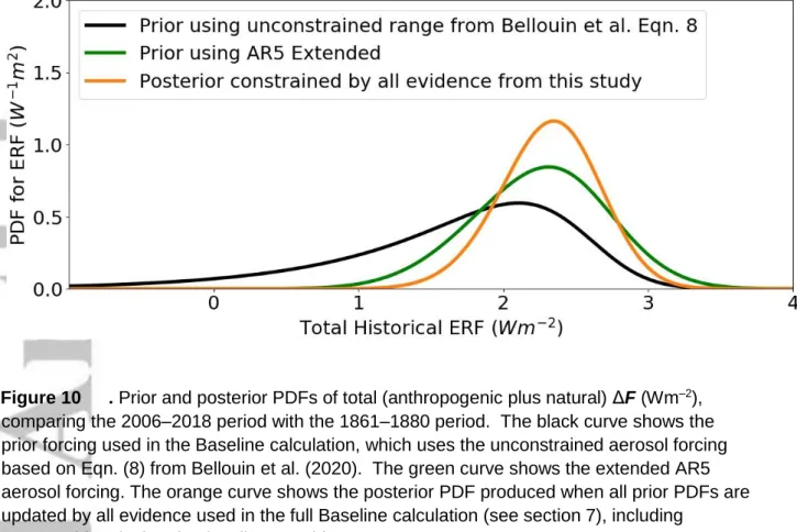
judgment using the available evidence about that quantity, without considering any other lines of evidence. These expert priors are given in the appropriate sections and are crucial in determining the historical and paleo likelihoods. Note that PDFs of these and other variables change once all the evidence is propagated through the model. For example, if historical warming turns out to be weaker than would be expected based on the other lines of evidence, then our posterior PDF of S shifts downward from what it would have been with only the other evidence—but at the same time, our posterior PDF of the historical ∆F also shifts downward relative to what we expected a priori. These revised, posterior PDFs will not be presented except those of S and the historical forcing ∆F.
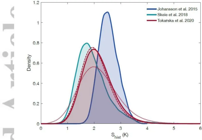
Many previous studies have used past climate changes to constrain climate sensitivity using Bayesian methods (e.g., Aldrin et al., 2012; Johannsen et al., 2015; 2018, Skeie et al., 2014; 2018), and so had to specify priors. Such studies mostly aimed to constrain S without incorporating the process knowledge exploited here, instead fitting inference models formulated with S or λ as an independent variable. As such, they required prior PDFs for S (which were typically uniform in S or peaked at S values somewhere within the 1.5-4.5 K range). Due to the use of a different inference model, the prior on S in this assessment is nominally based on less information and hence not fully equivalent to those in the past Bayesian ECS studies. This and other issues of how to interpret the priors are taken up in section 7.2.
2.4.4 Calculation of likelihoods and sampling method
Implementation of the Bayesian updating generally follows the principles described in Liu (2004), in which we sample from our prior over Φ and weight each instance in the sample according to the likelihood P(E|Φ). The weighted ensemble is then an approximation to the posterior PDF, and can be analyzed and presented as desired (e.g., in terms of the
mean/expectation and credible intervals) via relationships such as expectation E[Φ|E] = Σ(wj
Φj) / Σ(wj) where Σ denotes a sum over all instances Φj from Φ and wj is the weight. This
approach can also be viewed as a specific form of Importance Sampling (Gelman et al., 2013) in which the prior is used as an initial ‘proposal’ distribution from which samples are drawn and subsequently weighted to estimate the target distribution.
To create the sample, we begin by sampling the independent variables according to their priors (e.g., uniform sample distribution for a uniform prior), and then use the inference model equations to calculate the values of each dependent variable (such as S) and the model outputs for each instance in the sample. This yields a sample population
approximating the PPD for all variables in Φ. Next, a weight wj for each instance j is
computed from the global likelihood function (which is a product of local likelihoods, cf. eq. (
11). Finally, the posterior PDF is approximated by the histogram of the weighted sample (see below).
For the individual-feedback process evidence (see section 3), the likelihood for each feedback component i is represented as a Gaussian function with mean μi and standard
deviation σi. Each sample instance j is accordingly given a likelihood weight for λij equal to
G(λij, μi, σi) where λij is the ith feedback value of the jth instance in the sample, and G(x,μ,σ) is
defined as the Gaussian N(μ,σ) function evaluated at x. The weights for the six feedbacks are multiplied to give the total likelihood weight for the individual-feedback evidence. In the
baseline case with a prior uniform in λi, the posterior after updating by this likelihood thus
approximates the anticipated Gaussian N(μi,σi), although we do not explicitly take advantage
of this relationship within the algorithm, in order to allow full generality. Similarly, an
“emergent constraint” likelihood is specified in terms of a Gaussian in total λ, evaluated G(λj,
μλ, σλ).
For the observed temperature change evidence (see sections 4 and 5), we consider a forward model in the basic form (cf. eq.
3):
ΔT= f(Φ’)
where the predicted temperature change ΔT is a function of the other model variables Φ’. The observed temperature change ΔTobs, which includes an uncertainty σe due to
measurement error and unforced variability, is interpreted as giving rise to a likelihood which takes the Gaussian form N(ΔT,σe) (Annan and Hargreaves, 2020). Thus the likelihood
assigned to any Φ’ is G(ΔT, ΔTobs, σe), which is the probability of the observed warming for a
given ΔT=f(Φ’). This value is maximized when ΔT is equal to ΔTobs and drops off rapidly as
the difference between ΔT and ΔTobs becomes large compared to σe. The exact forward
models used will differ from (
3) due to additional terms as previously mentioned, and are given in sections 4 and 5.
Likelihood weights for process (excluding emergent-constraint), emergent-constraint, historical, and paleoclimate evidence (separately for cold and warm periods) are calculated for each instance. These weights (or a subset thereof) are then multiplied together to give a single likelihood weight w for each member of the sample.
The posterior PDF for Φ can be calculated from the weighted sample distribution; marginal PDFs for variable subsets are calculated from the marginal sample distributions. For example, a posterior PDF for S is calculated as the histogram of S in the sample (i.e, the PPD), weighted by the corresponding likelihood weights—i.e., p(S | E)
∝
Σj∈Q wj, where theset Q contains all instances j whose Sj falls within a histogram bin centered on S—with
normalization. Posterior PDFs for any other variable in Φ are calculated similarly. The marginal likelihood function for any variable (e.g., S) is just the average weight w from the same histogram. Hence the marginal likelihood is equal to the PDF divided by the PPD.
Various approximations are made in the sampling calculations to make them less computationally expensive. The Baseline calculation initially samples each feedback
component uniformly and independently over the range U(–10,10) (see Figure 7.2). We also use an alternative prior which is calculated by weighting samples from the Baseline prior to give a PPD for S which is uniform from near zero to 20 K. This does not include zero because the Baseline prior covers a finite range U(–10,10). When calculating the posterior, to avoid wasted computational effort, we restrict the initial sample to absolute values for each feedback λi within a six standard-deviation range of the likelihood function for that
feedback. This does not affect the posterior PDF because the likelihood is effectively zero outside this range. The posterior calculation in section 7.2 with a uniform-S PPD uses a weighted version of an equivalent sample (and so also makes this approximation). This approximation enabled us to to produce stable 5-95% ranges with a Monte Carlo sample size of 2x10¹⁰. We also used kernel smoothing to produce satisfactorily smooth posterior