HAL Id: hal-03144847
https://hal.inria.fr/hal-03144847
Submitted on 17 Feb 2021
HAL is a multi-disciplinary open access
archive for the deposit and dissemination of
sci-entific research documents, whether they are
pub-lished or not. The documents may come from
teaching and research institutions in France or
abroad, or from public or private research centers.
L’archive ouverte pluridisciplinaire HAL, est
destinée au dépôt et à la diffusion de documents
scientifiques de niveau recherche, publiés ou non,
émanant des établissements d’enseignement et de
recherche français ou étrangers, des laboratoires
publics ou privés.
Control of negative feedback loops in genetic networks
Ismail Belgacem, Jean-Luc Gouzé, Roderick Edwards
To cite this version:
Ismail Belgacem, Jean-Luc Gouzé, Roderick Edwards. Control of negative feedback loops in genetic
networks. CDC 2020 - 59th Conference on Decision and Control, Dec 2020, Jeju Island, South Korea.
�hal-03144847�
Control of negative feedback loops in genetic networks
Ismail Belgacem
1Jean-Luc Gouz´e
2and Roderick Edwards
3Abstract— The oscillator made of a negative loop of two genes is one of the most classical motifs of genetic networks. We give solutions to control such an oscillator by modifying the synthesis rates. Our models are given by piecewise affine systems, and the control is qualitative, taking only two values. Thus, the necessary measurements for implementing this control only depend on the fact that some gene is expressed or not. Our first goal is to obtain sustained oscillations. Then we study the control by a sliding mode for negative ODE loops in general, to suppress sustained or damped oscillations. Finally, we introduced a general idea for creating sustained oscillations in systems with damped oscillations following a particular cycle of domains.
I. INTRODUCTION
The huge quantity of high-throughput experimental data has now made modeling a useful and compulsory tool for the study of biological genetic networks. Several formalisms exist (see the review [1]), from the very qual-itative Boolean modeling ([2]) to the exhaustive mass action chemical modeling of each of the elementary steps of the transcription translation processes [3]. In this paper, to build dynamical models, we will use classical ordinary differential equations or, most frequently, the (equally classical) Piecewise Affine (PWA) formalism made with discontinuous differential equations.
Due to the enormous progress in genetic manipu-lations, it is now becoming possible to act upon the expression of one gene at the transcriptional or trans-lational level. For example, biochemical inducers may interfere with the main gene transcription effectors, and, depending on the quantity of inducer injected in the medium, the expression of some gene may be slowed down. On the basis of this recent progress in experi-mental synthetic biology [4], [5], [6], we assume that synthesis rates can be controlled by the biologist.
The use of control in mathematical modeling of genetic networks is less classical because the experi-mental means are quite recent. Moreover, the classical 1 Mezaourou, Ghazaouet, Tlemcen 13041, Algeria.
2 Universit´e Cˆote d’Azur, Inria, INRAE, CNRS,
Sorbonne Universit´e, Biocore Team, Sophia Antipolis, France
3Dept. of Mathematics and Statistics, U. of Victoria, PO BOX 1700
STN CSC, Victoria, B.C., Canada V8W [email protected]
mathematical tools of control theory [7] are rarely appli-cable. The classical theory is exhaustively developed for linear systems, with either positive or negative control. However, the controlled systems obtained from genetic networks are often non-linear, and the control often has a sign, because of the positive nature of biochemical concentrations, for example, or because it is possible to add an inducer in the medium but not to take it away.
Moreover, the experimental control of gene expression must often be qualitative [8]: concentrations of proteins or expression of genes (on or off) are only qualitatively known, and the control itself often has only a few possible values. It is not possible to exert a control with good precision, depending on a variable measured with good precision, as is done in classical control theory.
This paper sheds some light on possible solutions to these difficult problems in the particular case of qualitative control of periodic oscillation. Some for-malisms and publications already exist using qualitative control. In the paper [9], the authors have controlled in a qualitative way one the most famous motifs of two-gene systems: the bistable switch, a positive loop of two genes inhibiting each other. The dynamics of this system is characterized by two alternative states, each with a stable attractor (and an unstable one between the two), and the system may switch between the states. In this paper, we will use slightly different techniques to control the other classical motif of two genes: the oscillator, a system consisting of a negative loop of two genes that can generate sustained or damped oscillations. Our aim for control will be to obtain real periodic behaviour, when the behaviour without control consists of damped oscillations converging toward an equilibrium. We con-sider PWA differential systems, and a qualitative control that only changes from domain to domain, and therefore is a constant within a rectangular domain. The resulting controlled system is therefore still a PWA system, and we use known tools for these systems to obtain our results. The control is multiplicative with respect to the synthesis rate, and must be positive. In [10], the authors address a similar problem with affine additive control and a unique threshold per variable. However, the control here is based on the calculation of the first return map or the Poincar´e map. The Poincar´e map (for the example
A B
Fig. 1. A negative loop.
taken) was special, which made it easy to compute the derivative of the first return map near the fixed point. In the general case this method is limited, especially when the dimension of the system is large (the computation of the first return map becomes very much more difficult or sometimes impossible).
Our work has some relation with theoretical qualita-tive control techniques used for piecewise-linear systems in the field of genetic regulatory networks ([9]). The ap-proach is also similar to the domain apap-proaches used in hybrid systems theory, where there are some (controlled) transitions between regions, forming a transition graph [11], [12].
II. THE GENETIC OSCILLATOR
As explained above, one main motif in biological feedback is the negative feedback loop, which is, in its simplest form, a negative loop with two genes: the first gene activates the production of the protein of the second gene, which inhibits the synthesis of the protein of the first (Fig.1).
The classical model for this negative loop is:
( ˙ x1= κ1h−(x2, θ2, n) − γ1x1 ˙ x2= κ2h+(x1, θ1, n) − γ2x2 (1)
where h+ and h− are the increasing or decreasing Hill functions:
h+(x, θ , n) = xn/(xn+ θn), h−(x, θ , n) = θn/(xn+ θn) .
The dynamical behaviour of this system is rather easy to study; if we suppose that θ1< κγ11; θ2<
κ2
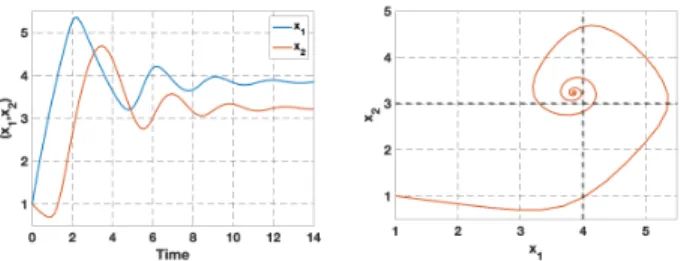
γ2 , then the system has oscillations. A classical study gives that there is a unique equilibrium, which is shown to be locally and globally stable (local stability is very easy because the trace of the Jacobian matrix is negative and the determinant is positive) [13]. Therefore the observed behaviour consists of damped oscillations converging to the equilibrium. An example simulation is given in Fig.2.
We are now interested in a qualitative description of this oscillator, corresponding to the case n → ∞ where the sigmoidal functions h+ and h− become step functions s+and s−. Without loss of generality, we will
Fig. 2. Oscillations for the system (1) with Hill functions (parameters κ1= 3, γ1= 0.25, κ2= 4, γ2= 0.5, θ1= 4, θ2= 3, x01= x02= 1).
consider only the case where the system is defined inside the (invariant) set [0, κ1/γ1] × [0, κ2/γ2]:
˙
x1 = κ1s−(x2, θ2) − γ1x1,
˙
x2 = κ2s+(x1, θ1) − γ2x2. (2)
This class of piecewise affine systems (PWA) was first introduced by L. Glass [14], and is widely used for modeling genetic regulatory networks [14], [15], [16], [17]. Step functions are not defined at threshold points, but solutions of the differential system on a threshold can still be defined in the sense of Filippov, as the solutions of differential inclusions.
The dynamics of system 2 can be divided into four regions, or domains, where the vector field is defined and very simple (linear):
B00 = {x ∈ R2≥0: 0 < x1< θ1, 0 < x2< θ2}
B01 = {x ∈ R2≥0: 0 < x1< θ1, θ2< x2< κ2/γ2}
B10 = {x ∈ R2≥0: θ1< x1< κ1/γ1, 0 < x2< θ2}
B11 = {x ∈ R2≥0: θ1< x1< κ1/γ1, θ2< x2< κ2/γ2}.
In addition, there are switching domains, where the system is defined only as a differential inclusion, cor-responding to the segments where each of the variables is at a threshold (xi= θi and xj ∈ [0, κj/γj]). We do
not need to use this approach here, because the vector fields from the two domains around the threshold are transverse to the segment, and therefore the solution of the differential equation is well defined.
In each of the regular domains, the analytic solution of decoupled linear (affine) equations can be obtained. To simplify the algebraic expressions that could become very long, we make the assumptions that the degradation rates are equal (which implies that trajectories are, in fact, straight lines, and simplifies the computations). Our methodology and the results would remain the same without this assumption.
Assumption 1: From now on, for sections II and III, γ1= γ2= γ.
y1 y2
y01 y11
Fig. 3. First-return map for system (2) with translated variables, starting from the boundary y1= y01< 0, y2= 0.
The study of such an oscillator has already been done [18]. We recall some results that will be use-ful for the stability analysis of this system. We now have four domains and four differential systems:
• in B( 00 ˙ x1= κ1− γx1 ˙ x2= −γx2 • in B( 10 ˙ x1= κ1− γx1 ˙ x2= κ2− γx2 • in B( 11 ˙ x1= −γx1 ˙ x2= κ2− γx2 • in B( 01 ˙ x1= −γx1 ˙ x2= −γx2
Within each domain, solutions converge toward a focal point outside of the domain; therefore the solution will cross the threshold and continue in the next domain. The possible transitions between domains are given by the transition graph (see [16] for explanations).
As in the continuous case, we add some constraints on the (positive) parameters to obtain oscillatory behaviour:
Assumption 2: θ1<κγ1 and θ2<κγ2
After a simple change of variables t0 = γt, y1 =
x1− θ1, y2= x2− θ2, we compute the first-return map
from one boundary (starting from the boundary y1=
y01< 0, y2= 0) of a domain to itself, see Fig.3.
The system being linear and decoupled (diagonal) within each domain, the computations are easy and have been done many times. The first return map is given by:
f(y1) = ρ y1 σ y1+ 1 , f0(y1) = ρ (σ y1+ 1)2 . (3) with, ρ = 1 and σ = θ−δ 1α β, δ = (θ1β + α β + θ1θ2+ α θ2), α =κγ1− θ1, β =κγ2− θ2, so that | f0(0)| = 1 and | f0(y
1)| < 1 ∀y1 (−θ1< y1< 0), so the point y1= 0
is locally and globally stable. We have the following proposition which is given in [18]:
Proposition 1: For a first return map of the form: ρ y
σ y + 1, (4)
Fig. 4. The behavior of the oscillator system (2) using the step function (parameters κ1= 2, κ2= 4, γ = 0.25, θ1= 4, θ2= 3, x01=
2, x02= 4).
if ρ ≤ 1, then the system is stable around y = 0; if ρ > 1 then there exists a stable limit cycle for y =ρ −1
σ .
Numerical simulations are given in Fig.4. III. THE GENETIC OSCILLATOR WITH CONTROL
To be able to control the system, we have first to define its outputs, i.e., the measurements that are available. Very often, classical control theory assumes that a measure of the real value x1or x2can be obtained
with good precision, and perhaps some noise. For ge-netic regulatory networks, the measurements are often qualitative or even Boolean, indicating only whether a gene is strongly or weakly expressed (see [19] for a review of experimental methods, such as microarrays or Western blots; see also [20]). In the framework of PWA systems, this means that we only know the domain (Bi j)
where the variables are, and not their precise values. Knowing this, a classical control (for example pro-portional to the variable) is not possible, and we can only fix a constant value for this control within each domain. This value may vary from domain to domain. We will suppose that the biologist is able to control, to some extent, the synthesis rate of one gene. It is a classical procedure, that can be done via the construction of a plasmid or by genetic modifications of the DNA strain to be able to act on the expression of the gene via an inducer. The goal of the control will be to obtain sustained oscillations, i.e., a periodic behaviour, as in [10].
If the control is on the synthesis rate of the first gene (for example), the new system is:
( ˙ x1= u(Bi j)κ1s−(x2, θ2) − γx1 ˙ x2= κ2s+(x1, θ1) − γx2 (5)
where Bi jis one of the four domains defined above. The
value of the control depends only on the domain; in two domains B01 and B11, the control is not active (has no
action on the system) because the function s−(x2, θ2)
system in these two regions. The control is only active in the other two regions, and may take two values; moreover, it should be positive.
In the following we will use a theorem in [21] to control the system. We recall this theorem (slightly adapted), which requires the following assumption.
Assumption 3: Pairs of successive focal points are aligned, i.e., in two successive focal points, at most one coordinate changes.
In this theorem (see [21]), the first return map T is defined from some wall (boundary between two domains ) W0 into itself, and DT(0) is the Jacobian matrix of T
evaluated at the equilibrium xi= θi.
Theorem 1: Let C = {a0, a1· · · a`−1} denote a
se-quence of regular domains that is periodically visited by the flow, and such that each domain ai has a unique exiting direction si. Suppose that the focal points of C
satisfy Assumption3, i.e., they are aligned. Suppose also that all variables are switching at least once.
Consider the first return map T : W0→ W0. Let λ =
ρ (DT(0)), the spectral radius of DT(0). Then, the following alternative holds:
i) if λ6 1, then ∀x ∈ W0, Tnx→ 0 when n → ∞. The
equilibrium is globally stable.
ii) if λ > 1 then there exists a unique nonzero fixed point q = Tq. Moreover, for every x ∈ W0\ {0},
Tnx→ q as n → ∞: the unique limit cycle is globally
stable for every solution starting away from the equilibrium.
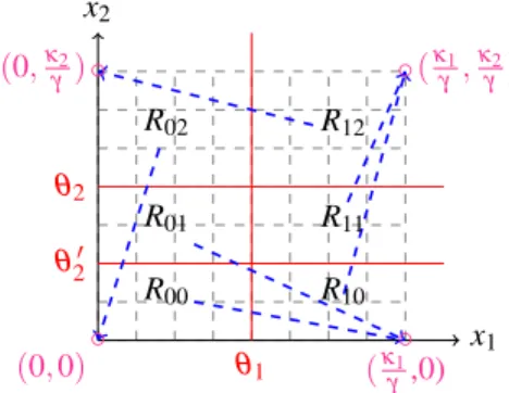
Suppose that two distinct thresholds are crossed in at least one direction. Then conclusion ii) holds (see [21]). To have two different thresholds in one direction for our system (5), we introduce an additional artificial threshold for one variable (x2= θ20 < θ2), see Fig. 5.
We now consider the system (6) with a control of the synthesis rate of the first variable, but we define now the control u in a more qualitative way, with the second threshold θ20< θ2. ( ˙ x1= u(Ri j)κ1s−(x2, θ2) − γx1 ˙ x2= κ2s+(x1, θ1) − γx2 (6)
We compute the focal point associated with each do-main (there are now 6 dodo-mains, Ri j, because there is one
more threshold for x2). The focal point associated with
each domain is given in the table. We have multiplied everything by γ to simplify.
C : R00 R10 R11 R12 R02 R01
u1κ1 u2κ1 u3κ1 0 0 u4κ1
0 κ2 κ2 κ2 0 0
(7)
We remark that now u may take at most four dif-ferent values (u1, u2, u3, u4) depending on the domain,
x1 x2 (0,κ2 γ ) (κ1 γ,0) θ2 θ20 θ1 R01 R00 R10 R11 R12 R02 ◦ ◦ ◦ ◦ (κ1 γ, κ2 γ) (0, 0)
Fig. 5. From each domain for system (6), solutions converge toward a focal point (circles) outside of the domain. The blue arrows represent the direction of vector fields from each region.
but remember that the focal points should be aligned and so we should take u1= u2. The focal points are
already aligned for the original system (without control), therefore we have to check the condition that each domain has a unique exit direction. We suppose that the usual assumptions for oscillatory behaviour are satisfied (see Assumption (2)), then we can see that all domains have a unique direction except R01 where starting from
an initial condition in this region we can go to R00, R10,
or R11, see Fig. 5.
We choose to apply a control in this region. We design a control u4as u4κ1/γ < θ1, to place the focal point of
R01 in the domain R00. With this choice, u has a low
value 0 < u4<γ θκ1
1 < 1 in R01 and the value u1= u2= u3= 1 (no control) in all other regions.
We now use Theorem1(see [21]) to show that, in our example, there is a unique stable limit cycle. A cycle C involving all regular domains exists for any param-eter set satisfying the specified constraints. Moreover, any pair of successive focal points only differ in the switching direction, i.e., assumption (3) is satisfied. The transition graph of the system with control is given in Fig.6. Hence, we may apply Theorem1, and since θ2
and θ20 are both crossed in C , we conclude that there exists a unique stable periodic orbit attracting all initial conditions, as shown in the simulation of Fig.7.
This control is very robust: the synthesis rate of one gene only has to be lowered sufficiently, the precise amount is not important. Moreover, the precise value of the second threshold θ20 for the design of the control has very light constraints (only θ20< θ2).
R00 R10
R11
R12
R02
R01
Fig. 6. The transition graph for the controlled system (6).
Fig. 7. The limit cycle resulting from the chosen control of system (6), starting from two different initial conditions (2, 4) and (3.7, 3.2) and using the same parameter values in Fig.4. Here θ20= 2. The solid
red line is the periodic orbit.
IV. QUALITATIVE CONTROL FOR NEGATIVEODE
LOOPS
We now consider a slightly different problem. Models are given by an ODE, and we try to control them in a qualitative way. In the following we apply a sliding mode control for negative ODE loops in general. For the implementation of this kind of control in biological systems, see in [22], where design guidelines are devel-oped.
Example 1: First, take the negative loop with two genes as above, given by
( ˙ x1= uκ1h−(x2, θ2, n) − γ1x1 ˙ x2= κ2h+(x1, θ1, n) − γ2x2 (8)
Here, the degradation rates are no longer equal. This system has a unique positive equilibrium, x∗1, x∗2, under the classical assumptions: θ1<κγ1
1; θ2<
κ2
γ2.
Without control (u = 1), this equilibrium is globally asymptotically stable with oscillatory behaviour, as we have seen above (see also Fig. 8). To design a control that suppresses these oscillations, it is enough to take
u= α/h−(x2, θ2, n),
which transforms the system into a linearly stable system (α is a positive parameter) without oscillation, and
Fig. 8. Oscillations in system (8) without control (parameters κ1=
κ2= 1, γ1= γ2= 0.5, θ1= θ2= 1, n = 6). The black and green curves
are the nullclines, and the red and blue curves are solution trajectories.
Fig. 9. Sliding mode in system (8) with control; the three black curves are the three nullclines for u = u−, 1, u+. Parameters for control are
u−= 0.1, u+= 2. The blue, red and green curves are as in Fig.8.
moreover is a positive control. To implement it, however, we would need to measure precisely the state x2.
Instead, we look for a qualitative control u, depending only on simple regions, such that the controlled system has no oscillatory behaviour around the equilibrium. We design the control u with two values: a “low” value u− and a “high” value u+, such that u−< 1 < u+(of course, u= 1 corresponds to no control). The control will change if x1 is less than or greater than its equilibrium x∗1: if
x1> x∗1, then u = u−; if x1< x∗1, then u = u+.
On the boundary, the control is not defined, but the solution of the system is defined by the Filippov solution (see [23]). The goal is to obtain a stable sliding mode on the line x∗1.
First, to simplify, we make the assumption that u−is small enough so that the first nullcline of the system with u−is completely contained in the half-space x1< x∗1. The
condition for this is u−κ1/γ1< x∗1.
Then we study the existence (or not) of a sliding mode along the line x∗1. The study is elementary, and
Fig. 10. Sliding mode control as in Fig.9, with zoom around the equilibrium (x∗1, x∗2).
is done with a simple phase plane analysis of the signs of vector fields between the nullclines. In Figs. (8) and (9), we have shown the second nullcline in green (it does not depend on the control) and the three nullclines in black, for u−, u = 1, u+. In the left half-space, x1< x∗1,
the control is u+, and in the right half-space, x1> x∗1,
the control is u−. We denote by P the point at the intersection of the first nullcline for u+, and x∗1, the equilibrium of the uncontrolled system. Then there is a sliding mode on x1∗ below this point P. Above P on the boundary, the two vector fields have the same sign and cross from right to left. Moreover, any trajectory in the plane will end up on the sliding mode line.
On the sliding mode itself, we have x1= x∗1, and the
equation for x2is:
˙
x2= κ2h+(x∗1, θ1, n) − γ2x2,
which is a simple affine system converging to the equi-librium. Therefore the sliding mode converges towards the desired reference equilibrium. Fig.10shows a zoom of the phase portrait towards its equilibrium.
In the controlled system, there are no oscillations. We now apply the method in dimension three.
Example 2: Consider the negative feedback loop given in Fig. 11, where protein X1 produces X2, which
then produces X3, which in turn inhibits the production
of X1. We suppose that each species Xi is subject to
degradation γi and X1 has a small basal unregulated
synthesis rate δ .
Using the law of mass action kinetics, we obtain: ˙ x1= u f (x3) + δ − m1x1 ˙ x2= α1x1− m2x2 ˙ x3= α2x2− γ3x3, (9) where m1= γ1+ α1, m2= γ2+ α1and f (x3) = κ3 θ3n xn 3+θ3n represents a decreasing Hill function.
X1 α1 X2 α2 X3 a δ γ3
Fig. 11. Inhibition of the production of X1 by the product X3 in
Example (2). m1m2γ3 α1α2 x ∗ 3− δ f(x3) = κ3 θ n 3 xn 3+θ n 3 x3 x∗3
Fig. 12. A single point of equilibrium in system (9).
Without a control (u = 1) and at the equilibrium, we get the following equations:
f(x3) = κ3 θ3n xn3+ θ3n= m1m2γ3 α1α2 x∗3− δ .
To determine the equilibria we have to study the inter-sections of the two functions above, sketched in Fig.12, where we can see that a single equilibrium point exists.
The Jacobian matrix at the equilibrium is −m1 0 f0(x∗3) α1 −m2 0 0 α2 −γ3 , (10)
and the characteristic polynomial of the linearized sys-tem around the equilibrium point is
λ3+ (m1+ m2+ γ3)λ2+ ((m1+ m2)γ3+ m1m2)λ + m1m2γ3 + α1α2f0(x∗3) = 0, f0(x∗3) = κ3n x∗3n−1θ3n (x∗3n+ θ3n)2 ! .
Thus, for the equilibrium of system (9) to be locally stable, it is sufficient that:
(m1+ m2+ γ3)((m1+ m2)γ3+ m1m2) − m1m2γ3
− α1α2f0(x∗3) > 0.
The equilibrium is locally unstable when n is large and a limit cycle is obtained; see results of simulations for n = 3 and then, n = 10 in Fig.13.
Taking parameter values in Fig. 13, and n = 10, the equilibrium will be ((x∗1, x∗2, x∗3) = (1.13, 2.26, 6.32)). Therefore, as above, to suppress the oscillations in this
Fig. 13. Simulations of system (9) with parameter values κ3= 3, m1=
0.25, m2= 0.25, α1= 0.5, α2= 0.7, γ3= 0.25, θ3= 5, δ = 0.02, n = 3
in the left pane, n = 10 in the right pane, and x01= 1, x02= 1, x03= 0.5.
case (n is large), we design a control u with two values: a “low” value u−(here 0.1) and a “high” value u+(here 10). We apply the low control, u−, when x1> x∗1and the
high control, u+, when x1< x∗1. A simulation is given
in Fig.14.
The same method is applicable in n dimensions for a negative loop, but the precise proof has to be done. This is part of our current work.
V. CREATION OF OSCILLATION BY QUALITATIVE CONTROL
The results of [24] give conditions under which a piecewise-affine network can have a periodic orbit. It is often possible to exploit these results to design an experimentally feasible control for a system having a globally stable equilibrium to produce sustained oscilla-tions. Mathematically, all that is required is the presence in the cycle of a non-branching domain (i.e., a domain in the cycle that has only one possible exit wall). A qualitative control that is always effective is one that is applied only in the non-branching domain and pulls the focal point in that domain sufficiently close to the exit wall (without crossing the wall). Whether or not this is feasible in practice depends on the ability to turn on the control only in the relevant state (concentrations of proteins above or below threshold), and on the sign of the control term. This method applies to a large class of systems in arbitrarily large dimensions. Here we give only a simple three-variable example.
Example 3: ˙ x1= −γ1x1+ κ1s−(x3)u1 ˙ x2= −γ2x2+ κ2s+(x1)(1 + β s−(x2)s−(x3)) ˙ x3= −γ3x3+ κ3s+(x2)(1 + β s+(x1)s−(x3))
To be specific and to keep calculations simple, we take θi = 1, γi = 1 and κi = 32 for i = 1, 2, 3, and
β = 103. It can then be shown, by the method of [25],
Fig. 14. The simulation of the system (9) with a sliding mode control.
that for the uncontrolled system (u1= 1) there is a
damped oscillation following the sequence of states 000 → 100 → 110 → 111 → 011 → 001 → 000, and that trajectories from either 010 or 101 fall into this cycle. No states on the cycle are branching points in the state-space diagram. The eigenvalues of the Jacobian matrix of the Poincar´e map at the threshold intersection are λ =439±3
√ 20553
968 , or λ1≈ 0.8978 and λ2≈ 0.0092, so
the threshold intersection is a stable equilibrium. The idea of this control strategy applied to the 000 box is to pull the focal point from (32, 0, 0) closer to the threshold θ1= 1. Thus, if we take
u1=
(
1 + α, ifx1< θ1, x2< θ2
1, otherwise
then the control is effective if α > −12 is sufficiently small (i.e., sufficiently close to −12). This can be con-firmed, and the exact value of αccan be computed such
that for any −12< α < αc, the fixed point of the Poincar´e
map at the threshold intersection is unstable, and a stable periodic orbit through the cycle of boxes exists. Indeed, the Jacobian of the Poincar´e map is
43 484+ 7 22(1 + 3α) 5 44+ 1 2(1 + 3α) 7 22(1 + 3α) 1 2(1 + 3α)
and its dominant eigenvalue is > 1 when trace(A) − det(A) > 1, which occurs when α < αc= −271.
VI. CONCLUSION
A solution for creating a limit cycle in a two-gene sys-tem is given. Many extensions of this work are possible. The first one, as indicated, consists in a generalization of the result when the degradation rates γi are distinct.
This is easy because the theorem we use is also valid for distinct degradation rates. Then we can qualitatively control general two-dimensional ODE negative loops.
A more interesting generalization would be to consider an oscillator or other patterns in higher dimensions, as in the famous example of the repressilator [5]. No theoretical obstacle is visible to applying our technique. The problem is that, in dimension three, there is already a stable limit cycle without control in the PWA case. However, the control could be used to change the limit cycle (modify the amplitude or the period) or suppress it. Further work is needed to solve this interesting problem. Finally, we introduced a general idea for creating sustained oscillations in systems with damped oscillations following a particular cycle of domains, when at least one domain on the cycle has only one possible exit boundary. Unlike the simple 3-variable system studied here, in large systems, and systems with unequal degradation rates, some of the computations may need to be done numerically. To conclude, we think that problems of quantitative control (control within a domain) are a promising area of investigation, amenable to experimental application. For example, a biological application is to control the protein p53. In stressed conditions, the concentration of p53 starts to oscillate [26]. In fact, this happen because there is a negative regulation of p53 by another protein called Mdm2. Inappropriate activity of p53 with too high or too low concentrations can lead to various diseases, such as neurodegenerative disorders characterized by a neuronal loss like Alzheimer’s [27], or early embryonic lethality [28]. In this context, our control strategy to suppress sustained oscillations (above) is a useful tool in order to force a disrupted p53 − Mdm2 loop that exhibits extreme undesirable values of p53 to recover healthy homeostatic conditions.
REFERENCES
[1] H. de Jong, “Modeling and simulation of genetic regulatory systems : a literature review,” Journal of Computational Biology, vol. 9(1), 2002.
[2] R. Thomas, “Boolean formalization of genetic control circuits,” J. Theor. Biol., vol. 42, pp. 563–585, 1973.
[3] A. Kremling, “Comment on mathematical models which describe transcription and calculate the relationship between mrna and protein expression ratio,” Biotechnology Bioengineering, vol. 96, no. 4, pp. 815–819, 2007.
[4] T. Gardner, C. Cantor, and J. Collins, “Construction of a genetic toggle switch in escherichia coli,” Nature, vol. 403,n0 6767, 2000.
[5] M. B. Elowitz and S. Leibler, “A synthetic oscillatory network of transcriptional regulators,” Nature, vol. 403, no. 6767, p. 335, 2000.
[6] M. Tigges, T. T. Marquez-Lago, J. Stelling, and M. Fussenegger, “A tunable synthetic mammalian oscillator,” Nature, vol. 457, no. 7227, p. 309, 2009.
[7] E. D. Sontag, “Mathematical control theory, volume 6 of texts in applied mathematics,” 1998.
[8] E. Sontag, “Some new directions in control theory inspired by systems biology,” IET Systems Biology, vol. 1, no. 1, pp. 9–18, 2004.
[9] M. Chaves and J.-L. Gouz´e, “Exact control of genetic networks in a qualitative framework: the bistable switch example,” Auto-matica, vol. 47, no. 6, pp. 1105–1112, 2011.
[10] R. Edwards, S. Kim, and P. Van Den Driessche, “Control design for sustained oscillation in a two-gene regulatory network,” Journal of mathematical biology, vol. 62, no. 4, pp. 453–478, 2011.
[11] C. Belta and L. C. Habets, “Controlling a class of nonlinear sys-tems on rectangles,” IEEE Transactions on Automatic Control, vol. 51, no. 11, pp. 1749–1759, 2006.
[12] L. Habets and J. H. Van Schuppen, “A control problem for affine dynamical systems on a full-dimensional polytope,” Automatica, vol. 40, no. 1, pp. 21–35, 2004.
[13] I. Belgacem, “Modelling, analysis and control of biological networks,” Ph.D. dissertation, 2015.
[14] L. Glass and S. Kauffman, “The logical analysis of continuous, nonlinear biochemical control networks,” J. Theor. Biol., vol. 39, pp. 103–129, 1973.
[15] H. de Jong, J.-L. Gouz´e, C. Hernandez, M. Page, T. Sari, and J. Geiselmann, “Qualitative simulation of genetic regulatory networks using piecewise linear models,” Bull. Math. Biol., vol. 66, pp. 301–340, 2004.
[16] R. Casey, H. de Jong, and J. Gouz´e, “Piecewise-linear models of genetic regulatory networks: equilibria and their stability,” J. Math. Biol., vol. 52, pp. 27–56, 2006.
[17] M. Chaves, E. Sontag, and R. Albert, “Methods of robustness analysis for boolean models of gene control networks,” IEE Proc. Syst. Biol., vol. 153, pp. 154–167, 2006.
[18] L. Glass and J. Pasternak, “Stable oscillations in mathematical models of biological control systems,” J. Math. Biol., vol. 6, pp. 207–223, 1978.
[19] E. Klipp, R. Herwig, A. Kowald, C. Wierling, and H. Lehrach, Systems biology in practice: concepts, implementation and ap-plication. John Wiley & Sons, 2008.
[20] E. P. Gianchandani, J. A. Papin, N. D. Price, A. R. Joyce, and B. O. Palsson, “Matrix formalism to describe functional states of transcriptional regulatory systems,” PLoS computational biology, vol. 2, no. 8, p. e101, 2006.
[21] E. Farcot and J.-L. Gouz´e, “Limit cycles in piecewise-affine gene network models with multiple interaction loops,” International Journal of Control, vol. 41, no. 1, pp. 119–130, 2010. [22] F. Montefusco, O. E. Akman, O. S. Soyer, and D. G. Bates,
“Ultrasensitive negative feedback control: a natural approach for the design of synthetic controllers,” PloS one, vol. 11, no. 8, p. e0161605, 2016.
[23] A. F. Filippov, Differential equations with discontinuous right-hand sides: control systems. Springer Science & Business Media, 2013, vol. 18.
[24] L. Lu and R. Edwards, “Structural principles for periodic orbits in glass networks,” Journal of Mathematical Biology, vol. 60, pp. 513–541, 2010.
[25] R. Edwards, “Analysis of continuous-time switching networks,” Physica D, vol. 146, pp. 165–199, 2000.
[26] M. Maroto and N. Monk, Cellular oscillatory mechanisms. Springer Science & Business Media, 2008, vol. 641.
[27] A. Szybi´nska and W. Le´sniak, “P53 dysfunction in neurodegen-erative diseases-the cause or effect of pathological changes?” Aging and disease, vol. 8, no. 4, p. 506, 2017.
[28] C. A. Brady and L. D. Attardi, “p53 at a glance,” Journal of cell science, vol. 123, no. 15, pp. 2527–2532, 2010.