HAL Id: hal-00716183
https://hal.inria.fr/hal-00716183
Submitted on 10 Jul 2012
HAL is a multi-disciplinary open access
archive for the deposit and dissemination of
sci-entific research documents, whether they are
pub-lished or not. The documents may come from
teaching and research institutions in France or
abroad, or from public or private research centers.
L’archive ouverte pluridisciplinaire HAL, est
destinée au dépôt et à la diffusion de documents
scientifiques de niveau recherche, publiés ou non,
émanant des établissements d’enseignement et de
recherche français ou étrangers, des laboratoires
publics ou privés.
On the Effectiveness of Register Moves to Minimise
Post-Pass Unrolling in Software Pipelined Loops
Mounira Bachir, Albert Cohen, Sid Touati
To cite this version:
Mounira Bachir, Albert Cohen, Sid Touati. On the Effectiveness of Register Moves to Minimise
Post-Pass Unrolling in Software Pipelined Loops. HPCS 2012 : International Conference on High
Performance Computing & Simulation, Pr Waleed Smari, Jul 2012, Madrid, Spain. �hal-00716183�
On the Effectiveness of Register Moves to Minimise
Post-Pass Unrolling in Software Pipelined Loops
Mounira BACHIR
Universit´e Pierre et Marie Curie - LIP6 Paris - France
Email: [email protected]
Albert Cohen
Ecole Normale Sup´erieure - INRIA Paris, France
Email: [email protected]
Sid-Ahmed-Ali Touati
INRIA Sophia AntipolisNice, France Email: [email protected]
Abstract—Software pipelining is a powerful technique to
ex-pose fine-grain parallelism, but it results in variables staying alive across more than one kernel iteration. It requires periodic register allocation and is challenging for code generation: the lack of a reliable solution currently restricts the applicability of software pipelining. The classical software solution that does not alter the computation throughput consists in unrolling the loop a posteriori [12], [11]. However, the resulting unrolling degree is often unacceptable and may reach absurd levels. Alternatively, loop unrolling can be avoided thanks to software register renaming.
This is achieved through the insertion of move operations, but
this may increase the initiation interval (II) which nullifies the benefits of software pipelining. This article aims at tightly controling the post-pass loop unrolling necessary to generate code. We study the potential of live range splitting to reduce
kernel loop unrolling, introducing additional move instructions
without inscreasing the II. We provide a complete formalisation of the problem, an algorithm, and extensive experiments. Our algorithm yields low unrolling degrees in most cases — with no increase of the II.
Index Terms—Instruction Level Parallelism, Compiler,
Reg-ister Allocation, Software Pipelining, Loop Unrolling, Code Optimisation
I. INTRODUCTION
Our focus is on the exploitation of instruction-level paral-lelism (ILP) in embedded VLIW processors [11]. Increased ILP translates into higher register pressure and stresses the register allocation phase(s) and the design of the register files. In the case of software-pipelined loops, variables can stay alive across more than one kernel iteration, which is challenging for code generation and generally addressed through: (1) hardware support — rotating register files — deemed too expensive for almost embedded processors, (2) insertion of register moves with a high risk of reducing the computation throughput — initiation interval (II) — of software pipelining, and (3) post-pass loop unrolling that does not compromise throughput but often leads to unpractical code growth.
We investigate ways to keep the size of the generated code compatible with embedded system constraints without compromising the throughput benefits of software pipelining. Having a minimal unroll factor reduces code size, which is an important performance measure for embedded systems because they have a limited memory size. Regarding high performance computing (desktop and supercomputers), loop code size may not be important for memory size, but may be
so for I-cache performance. In addition to the minimal unroll factors, it is necessary that the code generation scheme for pe-riodic register allocation does not generate additional spill; the number of required registers must not exceed MAXLIVE [10] (the maximum number of values simultaneously alive).
When the instruction schedule is fixed then the circular lifetime intervals (CLI) and MAXLIVE are known. In this case, known methods exist for computing unroll factors: (1) Modulo Variable Expansion (MVE) [11], [12] which computes a minimal unroll factor but may introduce spill (since MVE may need more than MAXLIVE registers without proving an appropriate upper-bound); (2) Hendren’s heuristic [9] which computes a sufficient unroll factor without introducing spill, but with no guarantee in terms of minimal register usage or unroll factor; (3) the Meeting Graph framework [6] whose unroll factor is formally proven to minimize register usage (MAXLIVE), but which does not guarantee a minimal unroll factor.
In [3], [2], the authors claim that the loop unrolling minimisation (LUM) using extra remaining registers after a periodic register allocation is an efficient method to bring loop unrolling as low as possible — with no increase of the initiation interval (II). However, some kernel loops may still require high unrolling degrees. These occasional high unrolling degrees suggest it may be worthwhile to consider combining the insertion ofmove operations with kernel loop unrolling.
This article proposes a technique to minimise the unroll factor after periodic register allocation by inserting move
instructions without compromising the throughput benefits of software pipelining1. We study all the possible cases of adding
move operations without altering the initiation interval (II) for already software pipelined loops. This is done by splitting a chosen variable into two new variables at a given clock cycle if a free functional unit exists and can execute the addedmove
operation.
The paper is structured as follows. Section II discusses the limitations of using the interference graph for register alloca-tion and briefly recalls the use of circular lifetime intervals (CLI) for periodic register allocation. Section III presents the
1In general, insertingmoveinstructions during register allocation is paired
closest related work on code generation. Section IV illustrates our idea intuitively on simple examples. In Section V, we explain in more detail how it is possible to minimise loop unrolling through the insertion of extra moves. Section VI formally describes our exhaustive algorithm. In Section VII, we demonstrate the effectiveness of our approach in a stan-dalone tool by hightlighting the different results. Finally, we present our conclusion in Section VIII.
II. PERIODICREGISTERALLOCATION: INTERFERENCE GRAPH VSCIRCULARLIFETIMEINTERVALS Register allocation in many compilers performs the classical graph coloring method originally proposed by Chaitin [5]. The different nodes in the graph represent the different variables that are candidates for register allocation. Two nodes are connected by an arc if the corresponding live ranges variables are simultaneously alive. This graph is commonly called interference graph [5]. The register allocation attempts to find a k coloring of the interference graph. That is, an assignement of k colors to the nodes such as two connected nodes have different colors. If such coloring is found then it can map the k colors into registers. However, if the graph is not k-colorable, some nodes are removed from the interference graph until this latter becomes k-colorable. The removed nodes are spilled into the memory because they are not assigned to registers.
The interference graph representation of register allocation has some weaknesses. In fact, given a set of variables live ranges, the interference graph contains only the overlapping information of any two variables live ranges. By the way, it does not reveal the overlapping information for more than two variables and it does not provide the times of variables overlapping. The lack of this information between variables ovelapping may lead to some limitations.
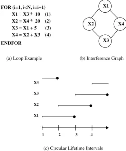
For instance, Chaintin’s register allocator may fail to find the minimum coloring even for simple loops. Figure 1(a) illustrates a simple loop program where MAXLIVE= 2 and
the traditional Chaitin’s [5] register allocator fails to find a register allocation with2 registers.
Some state-of-art work [6], [9] studied the circular lifetime intervals as an alternative representation for register allocation. Let us consider the interference graph given in Figure 1(b) which is similar to the one presented in [4]. Even though this graph is clearly 2-colorable, Chaintin’s heuristic fails because there is no node with degree < 2, and thus spill code has to
be introduced.
To address this problem, we represent in Figure 1(c) an alternative representation called circular lifetime intervals (CLI) [6], [13], [9]. The x-axis represents the different clock cycles and the y-axis represents the live ranges of the different variables. The barrier in the diagram represents the definition point of the variable while the arrow represents their last use. For example, variable X1 is defined at clock cycle 1 and
finishes at clock cycle3. Note that the lifetime of the variable
can span more than one iteration, as shown with variable
X4. Since the relation between the intervals is periodic, we
characterise this relation within one iteration.
X1 X2 X4
X3
(b) Interference Graph (a) Loop Example
1 2 3 4 X1 X2 X3 X4 X1 = X3 * 10 (1) X2 = X4 * 20 (2) X3 = X1 + 5 (3) X4 = X2 + X3 (4) ENDFOR
(c) Circular Lifetime Intervals
FOR (i=1, i<N, i=i+1)
Fig. 1. Interference Graph vs Circular Lifetime Intervals
Listing 1. Loop Program Example
FOR i=0, i<N, i=i+1 a[i+2] = b[i]+1 ; b[i+2] = c[i]+2 ; c[i+2] = a[i]+3 ; ENDFOR
As in any general graph coloring problem, finding the min-imum coloring of a circular lifetime intervals is NP-hard [8]. Many heuristics, exploiting the information provided in such representation are proposed in the litterature [6], [9]. The number of minimum registers needed for a circular interval is related to the width of the circular lifetime intervals. The main caracteristics related to circular lifetime intervals [9] are as follows:
• Two intervals I1, I2 are overlapping if there exists a clock cycle t where both of the intervals I1 and I2 are
simultaneously alive.
• The width of a given circular lifetime intervals F at time t, written as W idth(F, t), is the number of intervals
which are simultaneously alive at this time t.
• The maximum width of a given circular lifetime intervals
F , written as W(F ), is the maximum W idth(F, t), for all
clock cycle t∈ [0, II[. The maximum width is called also
MAXLIVE, the maximum number of variables which are simultaneously alive.
The following section reviews the main state-of-art periodic register allocation.
III. CODEGENERATION: BACKGROUND AND CHALLENGES
We review the main issues and approaches to code gener-ation for periodic register allocgener-ation using the loop example described in Listing 1.
Listing 2. Example of Register Renaming
FOR i=0, i<N, i=i+1
R3 = b[i]+1 ; b[i+2] = c[i]+2 ; c[i+2] = R1+3 ; R1 = R2 ; R2 = R3 ; ENDFOR
There are two ways to deal with periodic register allocation: using special architecture support such as rotating register
files, or without using such support. This latter may require
the insertion of moveoperations or loop unrolling
A. Rotating Register File
A rotating register file (RRF) [7] is a hardware mechanism to prevent successive lifetime intervals from being assigned to the same physical registers.
In Listing 1, variable a[i] spans three iterations (defined
in iteration i− 2 and used in iteration i). Hence, at least 3 physical registers are needed to carry simultaneously a[i], a[i + 1] and a[i + 2]. A rotating register file R automatically
performs the move operation at each iteration. R acts as a FIFO buffer. The major advantage is that instructions in the generated code see all live values of a given variable through a single operand, avoiding explicit register copying. Below R[k]
denotes a register with offset k from R.
Iteration i Iteration i+2
R=b[i]+1 ; R[+2]=b[i]+1 ;
b[i+2]=c[i]+2 ; b[i+2]=c[i]+2 ;
c[i+2]=R[-2]+3 ; c[i+2]=R+3 ;
Using a RRF avoids increasing code size due to loop unrolling, or to decrease the computation throughput due to the insertion of moveoperations.
B. Move Operations
This method is also called register renaming. Considering the example of Listing 1 for allocating a[i], we use 3 registers
and performmoveoperations at the end of each iteration [14], [15], [13]: a[i] in register R1, a[i + 1] in register R2 and a[i + 2] in register R3. Then we usemoveoperations to shift registers across the register file at every iteration as shown in Listing 2. However, it is easy to see that if variable v spans
d iterations, we have to insert d− 1 extramoveoperations at
each iteration. In addition, this may increase the II and may
require rescheduling the code if thesemoveoperations do not fit into the kernel. This is generally unacceptable as it negates most of the benefits of software pipelining.
C. Loop Unrolling
Another method, loop unrolling, is more suitable to maintain
II without requiring hardware support such as RRF. The
resulted loop body itself is bigger but no extra operations are executed in comparison with the original code. Here different
Listing 3. Example of Loop Unrolling
FOR i=0, i<N, i=i+3
R1 = b[i]+1 ; b[i+2] = c[i]+2 ;
c[i+2] = R2+3 ; R2 = b[i+1]+1 ;
b[i+3] = c[i+1]+2 ; c[i+3] = R3+3 ; R3 = b[i+2]+1 ; b[i+4] = c[i+2]+2 ; c[i+4] = R1+3 ;
ENDFOR
registers are used for different instances of the variable a of Listing 1. In Listing 3, the loop is unrolled three times. a[i+2]
is stored in R1, a[i + 3] in R2, a[i + 4] in R3, a[i + 5] in R1,
and so on.
By unrolling the loop, we avoid inserting extramove oper-ations. The drawback is that the code size will be multiplied by 3 in this case, and by the unrolling degree in the general case. This can have a dramatic impact by causing unnessary instruction cache misses when the code size of the loop happens to be larger than the size of the instruction cache. For simplicity, we did not expand the code to assign registers for b and c. In addition, brute force searching for the best solution using loop unrolling has a prohibitive cost, existing solutions may either sacrifice the register optimality [9], [12], [16] or incur large unrolling overhead [6], [17].
1) Modulo Variable Expansion: Lam designed a general
loop unrolling scheme called modulo variable expansion (MVE) [12]. In fact, the major criterion of this method is to minimize the loop unrolling degree because the memory size of the i-WARP processor is low [12]. The MVE method defines a minimal unrolling degree to enable code generation after a given periodic register allocation. This unrolling de-gree is obtained by dividing the length of the longest live range (maxvLTv) by the number of cycles of the kernel
α = ⌈maxvLTv
II ⌉. Once the loop is unrolled, MVE uses the
interference graph for allocation.
Having MAXLIVE the maximum number of values simul-taneously alive, the problem with MVE is that it does not guarantee a register allocation with minimal number of register equal to MAXLIVE [6], [9], and in general it may lead to unnecessary spills breaking the benefits of software pipelining. A concrete examples of this limitation can be found in [1]. In Listing 1, the longest live range lasts 8 cycles and the
number of cycles of the loop is3 cycles, so α = ⌈8
3⌉, and we should unroll the loop 3 times. Then we can assign to each variable a number of registers equal to the least integer greater than the span of the variable that divides II. In Listing 4, each variable a, b, c is assigned 3 registers using MVE: R1, R2,
R3 for a, R4, R5, R6 for b, R7, R8, R9 for c, and the loop is unrolled3 times.
One can verify that it is not possible to allocate the different variables on less than 9 registers when unrolling the loop 3
times. But MVE does not ensure a register allocation with a minimal number of registers, and hence it is not optimal. As we will see in the next section, we need 8 registers to
Listing 4. Example of MVE
FOR i=0, i<N, i=i+3
R1 = R5+1 ; R4 = R8+2 ; R7 = R2+3 ; R2 = R6+1 ; R5 = R9+2 ; R8 = R3+3 ; R3 = R4+1 ; R6 = R7+2 ; R9 = R1+3 ; ENDFOR
allocate the different variables. In MVE, the round up to the nearest integer for choosing the unrolling degree may miss opportunities for achieving an optimal register allocation.
2) Meeting Graphs: The algorithm of Eisenbeis et al.[6]
can generate a periodic register allocation using a minimal number of registers equal to MAXLIVE if the kernel is unrolled, thanks to a dedicated graph representation called the
meeting graph. It is a more accurate graph than the usual
interference graph, as it has information on the number of clock cycles of each variable lifetime and on the succession of the lifetimes all along the loop. It is based on circular lifetime intervals (CLI). A preliminary remark is that without loss of generality, we can consider that the width of the interval representation is constant at each clock cycle. If not, it is always possible to add unit-time intervals in each clock cycle where the width is less than MAXLIVE [6].
The formal definition of the meeting graph is as follows. Definition 1 (Meeting Graph). Let F be a set of circular
lifetime intervals graph with constant width r. The meeting graph related to F is the directed weighted graph G= (V, E). V is the set of circular intervals. Each edge e∈ E represents the relation of meeting. In fact, there is an edge between two nodes vi and vj iff the interval vi ends when the interval vj
begins. Each v∈ V is weighted by its lifetime length in terms of processor clock cycles.
The meeting graph (MG) allows us to compute an un-rolling degree which enables an allocation of the loops with
RC=MAXLIVE registers. It can have several connected
com-ponents of weights µ1, . . . , µk (if there is only one connected component, its weight is µ1 = RC), this leads to the upper
bound of unrolling α= lcm(µ1, ..., µk) (RC if there is only one connected component). Moreover a possible lower bound of loop unrolling is computed by decomposing the graph into as many circuits as possible and then computing the least common multiple (lcm) of their weights [6]. The circuits are then used to compute the final allocation. This method can handle variables that are alive during several iterations. This allocation always finds an allocation with a minimal number of registers (MAXLIVE).
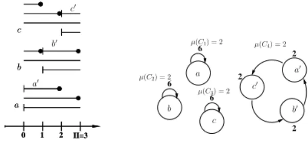
Figure 2(a) displays the circular lifetime intervals repre-senting the different variables (a, b, c) of the loop example described in Listing 1, the maximum number of variables simultaneously alive MAXLIVE = 8. As shown in
Fig-ure 2(b), the meeting graph is able to use 8 registers to allocate the different variables instead of 9 with Modulo Variable Expansion by unrolling the loop 8 times. For the
Listing 5. Example of Meeting Graph
FOR i=0, i<N, i=i+8
R1 = R2+1 ; R4 = R5+2 ; R7 = R7+3 ; R2 = R3+1 ; R5 = R6+2 ; R8 = R8+3 ; R3 = R4+1 ; R6 = R7+2 ; R1 = R1+3 ; R4 = R5+1 ; R7 = R8+2 ; R2 = R2+3 ; R5 = R6+1 ; R8 = R1+2 ; R3 = R3+3 ; R6 = R7+1 ; R1 = R2+2 ; R4 = R4+3 ; R7 = R8+1 ; R2 = R3+2 ; R5 = R5+3 ; R8 = R1+1 ; R3 = R4+2 ; R6 = R6+3 ; ENDFOR
loop described in Listing 1, the meeting graph generates the code shown in Listing 5.
0 1 2 II=3 0 1 2 II=3 8 8 8 a b c a b c b c a µ(C) =8+8+8 3 = 8
(a) Circular Lifetime Intervals (b) Meeting Graph
Fig. 2. Meeting Graph of the Loop Example in Listing 1 The main drawback of the meeting graph method is that the loop unrolling degree can be high in practice although the number of registers used is minimal. That may cause spurious instruction cache misses or even be impracticable due to the memory constraints, like in embedded processors. In order to minimise loop unrolling, Bachir et al. [2], [3] propose a method called loop unrolling minimisation (LUM method) that minimises the loop unrolling degree by using extra remaining registers for a given periodic register allocation. The LUM method brings loop unrolling as low as possible — with no increase of the II. However, some kernel loops may still require high unrolling degrees. This occasional cases suggest that it may be worthwhile to consider combining the insertion of moveoperations with kernel loop unrolling.
IV. SPLITTINGVARIABLESLIFETIMES: MOTIVATION As illustration in this section, we first present the simple example described in Figure 3 to illustrate the weaknesses of the loop unrolling minimisation (LUM method) described in [2], [3]. We then outline how these problems can be handled by addingmoveoperations.
Let us consider the two lifetime intervals a and b as described in Figure 3. Let us assume that the variable a is resulted from a multiplication and b is resulted from an addition. From these lifetimes, the corresponding meeting
0 1 2 3 4 5 4 1 5 6 4 0 1 2 3 4 II=5 b a′′ b a′ a′′ a′ a b µ(C1) =55= 1 µ(C2) =1+45= 1 µ(C1) =6+45 = 2 b
After Splitting the variable a into two variables a′and a′′at clock cycle c=II=5 a
Fig. 3. Splitting Variables Example
graph is drawn and has one circuit C1. The interval family has a width equal to the weight of the circuit C1 (µ(C1) = 2) and II = 5. Let us remind that the weight of this circuit
means that we need 2 registers to carry successfully the two
variables a, b if we unroll the loop twice (the code size is multiplied by 2) either if we use meeting graph framework or MVE technique.
If we want to not unroll the loop, we notice that the loop unrolling minimisation does not provide better loop unrolling degree bacause the minimal loop unrolling degree
α∗ ≥ maxi µ(Ci). In our example α∗ = µ(C1) = 2.
One possibility to reduce loop unrolling degree is called register renaming [15]. This latter proposes to allocate the variable a with 2 registers and perform move operation to carry the value from the first register to the second one. By the way, if we split the variable a into two variables (a′, a′′) where each spans less than one kernel iteration, then the problem of loop unrolling can be resolved.
In Figure 3, we assume that the adder unit is free at the clock cycle II. If we decide to split the variable a into two variables a′ and a′′ at the clock cycle II then we add only one moveoperation (a′′← a′) which is performed by using the free adder unit. The resulting allocation can be done with two registers as shown in Figure 3 without unrolling the loop (α∗= lcm(µ(C1), µ(C2)) = 1).
Another running example of splitting variables is represented in Figure 4. In fact, Figure 4 shows how to minimise the loop unrolling degree by splitting the variables of the circular lifetime intervals of Figure 2. In Figure 2(a), variable lifetimes are depicted by circular lifetime intervals. Each variable is alive during8 cycles, this means 3 iterations as II = 3. From
these lifetimes, the corresponding meeting graph is drawn in Figure 2(b). The interval family has a width equal to
µ(C) = 8. So hence, we need 8 registers to carry successfully
three variables a, b, c if we unroll the loop 8 times.
In Figure 4, we assume that adding one move operation at each clock cycle does not alter II. Each variable is splitted into one6 cycles interval and one 2 cycles interval. In Figure 4(a),
variable a is cut after 6 cycles and hence it results two
2 0 1 2 II=3 0 1 2 II=3 2 2 6 6 6 c′ b′ a b c a b c a b c a′ b′ c′ a′ µ(C4) = 2 µ(C1) = 2 µ(C3) = 2 µ(C2) = 2
(a) Circular Lifetime Intervals After Splitting Variables (b) Meeting Graph After Splitting Variables
Fig. 4. Running Splitting Variables Method on Circular Lifetime Intervals described in Figure 2
Listing 6. Final Register Allocation After Splitting Variables
FOR i=0, i<N, i=i+2 R3 = R2+1 | R2 = R3 ; R5 = R1+2 | R1 = R5 ; R7 = R2+3 | R2 = R7 ; R4 = R1+1 | R1 = R4 ; R6 = R2+2 | R2 = R6 ; R8 = R1+3 | R1 = R8 ; ENDFOR
variables a and a′, variable b is cut at clock cycle7 generating two variables b and b′ and variable c is cut at clock cycle 8 and hence it results two variables c and c′. The corresponding meeting graph is drawn in Figure 4(b). The three variables
a′, b′, c′ are allocated on R1, R2, by unrolling the loop twice. The copies of variable a (resp. b and c) are allocated
on R3, R4 (resp. R5, R6 and R7, R8). The final register
allocation is shown in Listing 6, where S1|S2denotes that S1 and S2 are executed in parallel.
The following section describes in details the exhaustive solution to minimise the loop unrolling degree by splitting variables without increasing the computation throughput.
V. SPLITTINGVARIABLES TOMINIMISELOOP UNROLLINGDEGREE
The impact of a loop register allocation scheme can be measured by 3 parameters. The first one is the number RC of allocated registers. A lower bound for RC is the
maximal number of simultaneously alive variables, denoted as MAXLIVE. The second one is the unrolling degree α. Large unrolling degrees are induced by the fact that a least common multiple (lcm) is computed. Roughly speaking, if you must unroll p times for one set of variables and q times for another one, then you have to unroll at least lcm(p, q)
times. When we use the loop unrolling minimisation (LUM method) by using the remaining registers [2], [3], the minimal loop unrolling degree can still be high. This is due to the formulation of the LUM method which proposes to update the different circuits weights µ1, . . . , µk generated by the meeting graph by adding the remaining registers. The resulting final loop unrolling degree α∗ is greater or equal to the maximum circuit weight (α∗>= max(µ1, . . . , µk)).
This paper proposes to find a periodic register allocation with a small circuit weights which leads to a small lcm. Our exploratory method consists in splitting the different variables by adding m extramoveinstructions. The impact of this third parameter is hard to measure because sometimes the added
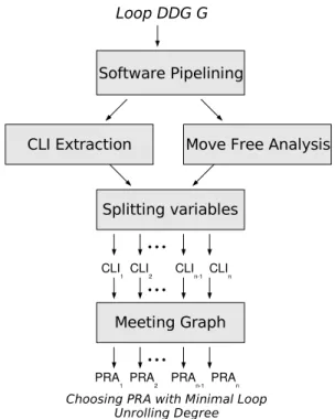
move instructions can be executed in parallel with the other operations. Based on these parameters our study follows these different phases:
1) Consider a software pipelined loop
2) Find the number of free functional units at each clock cycle which executemoveinstruction while preserving the Initiation Interval (II)
3) Extract the circular lifetimes intervals (CLI) from the software pipelined loop devoted to be allocated by the meeting graph
4) Compute all the possible combinations of splitting the different variables of CLI following the number of possiblemoveat each clock cycle
5) For each configuration of splitting variables, compute the periodic register allocation and then choose the one with the minimal loop unrolling degree
Step 2 aims to collect information about the number of
move operations at each clock cycle that can be executed without altering II. Once this information available, step 4 computes all possible splitting variables following the number of possiblemoveoperations at each clock cycle. Each splitting variable generates a new CLI. Finally, having all the different CLIs, we perform for each one the periodic register allocation using the meeting graph technique and then we choose the best CLI with the minimal loop unrolling degree.
Figure 5 portrays all the different steps. An arrow between two phases means that the target phase needs the information of the source phase. We note CLI for Circular Lifetimes Intervals and PRA for Periodic Register Allocation (PRAi means the meeting graph of the ith CLI).
VI. EXHAUSTIVESEARCHALGORITHM
In this section, we explain our exhaustive algorithm to find a periodic register allocation with a minimal loop unrolling size. First of all, we assume that we have the initial circular lifetimes intervals (CLI) and we provide the number of possible added
move instructions at each clock cycle t = 0, II − 1. These move instructions, if added, can be executed in parallel with other operations without altering II. In our study, the number of possible added moveinstructions at each clock cycle t is denoted mt and computed as mt = max(0, MAXMOVE − deft)
Where MAXMOVE is the number of functional units per-formingmoveoperations and deftis the number of variables which are defined at clock cycle t.
In order to compute all the possible cases of splitting variables for a given CLI, we look for the number of variables which can be splitted at each clock cycle t. In fact, a variable
v can be splitted into two variables v′ and v′′ at clock cycle
t as explained in the following definition.
Fig. 5. Splitting Variables to Minimise Loop Unrolling
Definition 2 (Splitting Variable). Let CLI be a circular lifetime
intervals and let the variable v ∈ CLI. Let us consider two
functions S and E such as
• S(v) is the start time of v (definition time) and • E(v) is the end time of v (the last used time).
The variable v is splitted into two variables v′, v′′ at clock
time t iff and only iff S(v) < t < E(v). The resulting variables v′ and v′′have the following lifetimes:
• S(v′) = S(v) and E(v′) = t
• S(v′′) = (t mod II) and E(v′′) = E(v) − t
When the variable v is splitted, new circular lifetime inter-vals called Result is created such as:
Result= {l ∈ CLI | l <> v} ∪ {v′, v′′}
From Definition 2, the number wt of variables which can be splitted at clock cycle t is the number of variables which are alive but not defined at this clock cycle. Let us assume that
W idth(CLI, t) is width of CLI at clock cycle t and deft is the number of variables which are defined at this clock cycle then the number of variables which can be splitted at time t is as wt= W idth(CLI, t) − deft
Consequently, for a given CLI and a given time t, we can split at most mt variables among wt alives one. That is, we can decide either to not split any variable (saving the original CLI) or to split 1 variable among wt variables (generating
C1
wt possible CLIs) or to split2 variables among wtvariables
(generating C2
wt possible CLIs) or . . . or to split mtvariables
among wt ones (generating Cmt
wt possible CLIs). As results,
the set of generated CLIs for a given CLI at time t denoted
Gt, is the sum of the different combinations Ci
the number of variables which we want to split and wt the number of maximum splitted variables at time t. That is, the cardinal of the set Gtis as follows:
|Gt| = mt X i=0 Ci wt
Furthermore, if we have k different CLIs at time t then we generate for each CLI, Pmt
i=0C i
wt CLIs. So hence, the total
number of generated CLIs at time t is k×Pmt
i=0C i wt.
In order to find the set G of all possible splitting variables configurations, we need to store the results of splitting vari-ables at each clock cycle t, which are then reused later at cycle = t + 1, II − 1. In fact, we need this new CLIs to
compute further splitting configurations. Formally, the cardinal of the set G of all possible splitting variables configurations is as follows: |G| = II−1Y t=0 mt X i=0 Cwit
Algorithm 1 implements our exhaustive search for splitting variables following possible added move intructions. In this algorithm, we require the initial CLI, the initiation interval
II and the information mt about available units at each
clock cycle t. This algorithm returns all the possible splitting variables configurations (CLIs) which are stored in the set G by computing the different combinations. In fact, at time t, splitting i variables among wtvariables (the generation of Cwit
CLIs) consists in splitting one variable for the different CLIs generated by splitting (i − 1) variables among wt variables (the already generated Ci−1
wt CLIs). That is, at time t, we use
two other sets Gc which contains the CLIs resulting from a given combination (Ci
wt) and the set Gt which contains the
CLIs resulting from the previous combination Ci−1
wt or which
initially contains the generated CLIs at clock time t− 1.
As we can see in Algorithm 1, the principal algorithm calls the sub-algorithm SPLIT-VARIABLE with the following parameters: the given CLI, the variable v which we want to split into two variables, the cycle window where exactly we want to split the variable v (variable v can span more than one kernel iteration). This sub-algorithm returns the generated CLI called Result and a boolean equal to TRUE if the variable v is actually splitted at clock cycle window, FALSE otherwise. Algorithm 1 delivers all the possible splitting configurations in finite time because it is dominated by the number of generated CLIs: QII−1t=0 Pmt
i=0C i wt
VII. EXPERIMENTALRESULTS
To study the efficiency of our empirical study, we developed a standalone tool to generate all the possible new CLIs following the number of possible move operations at each clock cycle and then perform for each generated CLI the meeting graph framework in order to find the periodic register allocation with a minimal loop unrolling.
We did extensive experiments on1935 CLIs extracted from
various known benchmarks, namely Livermore loops, Linpack
Algorithm 1 Splitting Variables Algorithm
Require: CLIinit , II and at each clock cycle t the number of
possible addedmovemt without atering II
Ensure: The set G of all the possible generated CLIs
G← {CLIinit} {G contains the initial CLI}
for t= 0 to II− 1 do
Gt← G {Gt contains all generated CLIs at time t− 1}
while mt<>0 do
Gc ← ∅ {initialisation of Gc which contains the generated
combination Ci
wt of CLIs (i= 0, mt)}
for each CLI∈ Gt do
for each v∈ CLI do
window← t {variables spanning more than one
itera-tion}
while window < E(v) do
if SPLIT-VARIABLE(CLI, v, window, Result)
then Gc← Gc∪ {Result} end if window← window + II end while end for end for G← G ∪ Gc; Gt← Gc ; mt← mt− 1 end while end for RETURN(G)
and Nas. In our experiments, the processor has one functional unit which can execute move operations (adder unit).
In order to have an idea about the complexity of the exhaus-tive solution, we draw in Table I the number of experimented CLIs for each benchmarks, the number of CLIs where it is possible to add move operation and the number of generated CLIs needed to find the best CLI with a minimal number of registers.
Table I shows that from1935 CLIs, there are only 343 CLIs
where it is possible to add move operations without increasing
II. The number of the generated CLIs is 108934. On average,
the running time of our exhaustive solution on a dual core 2 GHz Linux PC is 272 milli-seconds. The maximal observed runtime of Algorithm 1 is about 84 seconds.
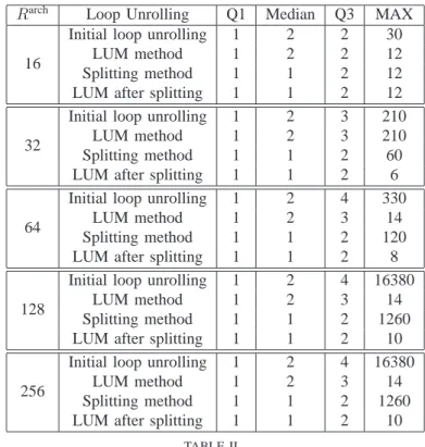
In order to highlight the improvements of splitting variables to minimise loop unrolling, we performed a periodic register allocation for each generated CLI and then compared the initial loop unrolling before splitting and the minimal loop unrolling after splitting. In addition, we wanted to know if the loop unrolling minimisation method (LUM method) described in [2], [3] provides lower loop unrolling.
In these experiments, we take into account only CLIs where it is possible to add move operations. We varied the number of architectural registers (Rarch) from16 to 256 registers. Table II
displays for each method the following observations : the lower quartile (Q1 = 25%), the median (Q2 = 50%), the
upper quartile (Q3 = 75%), and the largest loop unrolling
degree (max). Furthermore, we use for comparison the initial
loop unrolling, the final loop unrolling using the loop unrolling minimisation (LUM method), the final loop unrolling using splitting variables and final loop unrolling using splitting
Benchmarks Initial Possible Splitting Generated
CLIs CLIs CLIs
Alvinn 19 0 0 Applu 82 6 42 Appsp 106 14 177 Buk 34 0 0 Cgm 22 2 6 Doduc 23 1 701 Ear 55 7 48 Embar 22 0 0 Eqntott 37 4 15 Espresso 202 52 160 Fpppp 17 4 171 Gcc 270 53 187 Hydro2d 226 16 1339 Li 25 4 10 Linpack 27 4 9 Livermore 29 3 20 Mdljdp2 49 2 24 Mdljsp2 12 0 0 Mgrid 48 5 14 Nasa7 47 0 0 Ora 6 0 0 Random 320 137 103236 Sc 65 5 24 Spice2g6 104 12 38 Su2cor 10 2 8 Tmp 58 8 2663 Tomcatv 18 2 40 Wave 2 0 0 Sum total 1935 343 108934 TABLE I
INITIALCLIS,THE POSSIBLE SPLITTINGCLIS AND THE GENERATED SPLITTINGCLIS
variables method followed by the LUM method.
From the different results, we remark that adding move operations decreases dramatically the initial loop unrolling degree. Actually, thanks to splitting method, we do not unroll
50% of loops and at most we unroll twice 75% of loops.
We also see in Table II that combining the loop unrolling minimisation method with splitting method decreases greatly the maximum loop unrolling degree. For example, in a given machine with 64 registers, we minimise the loop unrolling from 330 to 8.
VIII. CONCLUSION
Minimising loop unrolling by using extra remaining reg-isters is an efficient method to reduce unroll factors for periodic register allocation. However, some real-world loops still require high unrolling degrees [3], [2]. This occasional cases suggest that it may be worthwhile to combine the insertion of moveoperations with kernel loop unrolling.
Rarch Loop Unrolling Q1 Median Q3 MAX
16
Initial loop unrolling 1 2 2 30
LUM method 1 2 2 12
Splitting method 1 1 2 12
LUM after splitting 1 1 2 12
32
Initial loop unrolling 1 2 3 210
LUM method 1 2 3 210
Splitting method 1 1 2 60
LUM after splitting 1 1 2 6
64
Initial loop unrolling 1 2 4 330
LUM method 1 2 3 14
Splitting method 1 1 2 120 LUM after splitting 1 1 2 8
128
Initial loop unrolling 1 2 4 16380
LUM method 1 2 3 14
Splitting method 1 1 2 1260 LUM after splitting 1 1 2 10
256
Initial loop unrolling 1 2 4 16380
LUM method 1 2 3 14
Splitting method 1 1 2 1260 LUM after splitting 1 1 2 10
TABLE II
STATISTICS ON LOOP UNROLLING WHEN AT MOST ONE MOVE IS ADDED PER CLOCK CYCLE
We study the potential for live range splitting to reduce kernel loop unrolling, describing how to introduce newmoves without inscreasing II. Moreover, we show that an exhaustive solution for splitting variables can produce satisfactory results. For example, when we assume that we can add at most one
move operations per cycle, then half of the loops do not need to be unrolled and 25% more need an unroll factor of 2. In addition, the maximun loop unrolling is highly reduced while combining splitting variables method with loop unrolling minimisation method.
In most cases, our method is a satisfactory solution to gener-ate compact code after periodic register allocation. Neverthe-less, we noticed that some loops still require high unrolling degrees despite our optimisation. This shows that optimal exploitation of remaining registers plus the insertion of II-preserving moves may not always be sufficient to bring the unroll factor down to acceptable levels. This provides an interesting fundamental limit of the applicability of software pipelining without hardware support for rotating register files.
REFERENCES
[1] Mounira Bachir. Loop Unrolling Minimisation for Periodic Register
Allocation. PhD thesis, Universit´e de Versailles Saint-Quentin-En-Yvelines, France, 2010.
[2] Mounira Bachir, David Gregg, and Sid-Ahmed-Ali Touati. Using the meeting graph framework to minimise kernel loop unrolling for scheduled loops. In Proceedings of the 22nd International Workshop
on Languages and Compilers for Parallel Computing, Delaware, USA,
[3] Mounira Bachir, Sid-Ahmed-Ali Touati, and Albert Cohen. Post-pass periodic register allocation to minimise loop unrolling degree. In LCTES
’08: Proceedings of the 2008 ACM SIGPLAN-SIGBED conference on Languages, compilers, and tools for embedded systems, pages 141–150,
New York, NY, USA, 2008. ACM.
[4] P. Briggs, K. D. Cooper, K. Kennedy, and L. Torczon. Coloring heuristics for register allocation. In PLDI ’89: Proceedings of the
ACM SIGPLAN 1989 Conference on Programming language design and implementation, pages 275–284, New York, NY, USA, 1989. ACM.
[5] Gregory Chaitin. Register allocation and spilling via graph coloring.
SIGPLAN Not., 39(4):66–74, 2004.
[6] Dominique de Werra, Christine Eisenbeis, Sylvain Lelait, and Elena Stohr. Circular-arc graph coloring: On chords and circuits in the meeting graph. European Journal of Operational Research, 136(3):483–500,
February 2002.
[7] James C. Dehnert, Peter Y.-T. Hsu, and Joseph P. Bratt. Overlapped loop support in the cydra 5. In ASPLOS-III: Proceedings of the
third international conference on Architectural support for programming languages and operating systems, pages 26–38, New York, NY, USA,
1989. ACM.
[8] M. R. Garey, D. S. Johnson, Gary L. Miller, and C. H. Papadimitriou. The complexity of coloring circular arcs and chords. SIAM J. Alg. Disc.
Meth., 1(2):216–227, June 1980.
[9] Laurie J. Hendren, Guang R. Gao, Erik R. Altman, and Chandrika Mukerji. A register allocation framework based on hierarchical cyclic interval graphs. In CC ’92: Proceedings of the 4th International
Conference on Compiler Construction, pages 176–191, London, UK,
1992. Springer-Verlag.
[10] Richard A. Huff. Lifetime-sensitive modulo scheduling. SIGPLAN Not., 28(6):258–267, 1993.
[11] P. Faraboschi J. A. Fisher and C. Young. Embedded Computing: a VLIW
Approach to Architecture, Compilers and Tools. Morgan Kaufmann Publishers, 2005.
[12] M. Lam. Software pipelining: an effective scheduling technique for vliw machines. SIGPLAN Not., 23(7):318–328, 1988.
[13] Sylvain Lelait, Guang R. Gao, and Christine Eisenbeis. A new fast algorithm for optimal register allocation in modulo scheduled loops. In
Proceedings of the 7th International Conference on Compiler Construc-tion, pages 204–218, London, UK, 1998. Springer-Verlag.
[14] Josep Llosa and Stefan M. Freudenberger. Reduced code size modulo scheduling in the absence of hardware support. In Proceedings of the
35th annual ACM/IEEE international symposium on Microarchitecture,
MICRO 35, pages 99–110, Los Alamitos, CA, USA, 2002. IEEE Computer Society Press.
[15] Alexandru Nicolau, Roni Potasman, and Haigeng Wang. Register allocation, renaming and their impact on fine-grain parallelism. In
Proceedings of the Fourth International Workshop on Languages and Compilers for Parallel Computing, pages 218–235, London, UK, 1992.
Springer-Verlag.
[16] B. R. Rau, M. Lee, P. P. Tirumalai, and M. S. Schlansker. Register allocation for software pipelined loops. SIGPLAN Not., 27(7):283–299, 1992.
[17] Sid-Ahmed-Ali Touati and C. Eisenbeis. Early Periodic Register Allocation on ILP Processors. Parallel Processing Letters, 14(2):287– 313, 2004.