HAL Id: halshs-00590828
https://halshs.archives-ouvertes.fr/halshs-00590828
Preprint submitted on 5 May 2011HAL is a multi-disciplinary open access archive for the deposit and dissemination of sci-entific research documents, whether they are pub-lished or not. The documents may come from
L’archive ouverte pluridisciplinaire HAL, est destinée au dépôt et à la diffusion de documents scientifiques de niveau recherche, publiés ou non, émanant des établissements d’enseignement et de
Ambition and jealousy. Income interactions in the ”Old”
Europe versus the ”New” Europe and the United States
Claudia Senik
To cite this version:
Claudia Senik. Ambition and jealousy. Income interactions in the ”Old” Europe versus the ”New” Europe and the United States. 2007. �halshs-00590828�
P
ARIS-JOURDAN
S
CIENCES
E
CONOMIQUES
48,BD JOURDAN –E.N.S.–75014PARISTEL. :33(0)143136300 – FAX :33(0)143136310 www.pse.ens.fr
WORKING PAPER N° 2005 - 14
Ambition and jealousy. Income interactions in
the "Old" Europe versus the "New" Europe and the United States
Claudia Senik
JEL Codes: C23, D63, O57, C25
Keywords: income distribution, comparison income, subjective well-being, Transition, European Union, panel data
AMBITION AND JEALOUSY.
INCOME INTERACTIONS IN THE “OLD”EUROPE VERSUS THE “NEW”EUROPE AND THE
UNITED STATES
First version October 2005 This version March 2, 2007
Claudia Senik*
Abstract Using individual-level data from a large number of countries, this paper examines how self-reported subjective well-being depends on own income and reference income, where reference income is defined as the income of my professional peers. It uncovers a divide between “old” -low mobility- European countries versus “new” European post-Transition countries and the United States. Whereas in the old Europe, the income of my reference group exerts a negative effect on my individual welfare, it has a positive impact in the new Europe and the United States. This finding is interpreted as reflecting the relative importance of comparisons (“jealousy”) versus information (“ambition”), which in turn depends on the degree of mobility and uncertainty in the economy.
Key words: income distribution, comparison income, subjective well-being, Transition, European Union, panel data.
JEL classification: C23, D63, O57, C25,
*Claudia Senik
Paris School of Economics Université Paris IV Sorbonne,
PSE (UMR CNRS, EHESS, ENPC, ENS), Institut Universitaire de France and IZA 48, bd Jourdan, 75014 Paris, France
Tel: 33-1-43-13-63-12 e-mail: senik@pse.ens.fr
In modern democracies, income inequality is certainly one of the issues that most strongly divide the population into constituencies for different political parties. On what grounds are these political attitudes based: self-centered interests or concerns for others, benevolence or envy? This paper is one of a series that investigate the subjective perception of income distribution (e.g. Piketty, 1995, Benabou and Ok, 2001, Alesina et al., 2001, 2004, 2005, Corneo and Gruner, 2000, Ravallion and Lokshin, 2001, Fong, 2001, 2004; see Senik (2005a) for a survey). From a subjective point of view, income distribution has two dimensions. One is income inequality in general, i.e. the distribution of aggregate income. The other is the gap between my own income and that of some relevant other: when the income of, say, my colleagues raises above mine, what is the consequence on my welfare? This paper is dedicated to this question.
It explores the idea that the difference between my own income and that of a reference group can be interpreted in two different ways, and accordingly, have two opposite welfare effects: relative deprivation versus welfare enhancing “anticipatory feelings” (Caplin and Leahy, 2001). Hirschman (1973) dubbed the latter the “Tunnel Effect”. The idea is that individuals can derive
positive flows of utility from observing other people’s faster progression if they interpret this movement as a sign that their turn will come soon, for instance if the other lane of cars starts progressing towards the exit while their lane is still immobile during a traffic jam inside a tunnel1. In mundane words, the objective of this paper is thus to elucidate empirically the
following question: when it comes to one’s relative position on the income ladder, which is the dominant passion: jealousy or ambition?
It is important to distinguish these two different types of social interactions (see Manski and Straub, 2000) because they imply different policy measures: comparison effects constitute an argument for measures that equalize income or consumption, whereas the prospect for mobility does not. Income comparisons have many other consequences that cannot be derived from informational learning; in particular, they call into question the relevance of growth as an objective of economic policy, and as an aggregate measure of welfare (Frank, 1997, Lungqvist and Uhlig, 2000, Cooper et al., 2001, Easterlin, 2003; see Luttmer (2005) for a more extensive list). Whether ambition dominates jealousy or not is thus a matter of interest for economic policy.
This paper argues that both types of interactions always coexist but that their respective importance depends on the degree of mobility and uncertainty of the economic environment, as perceived by a country’s inhabitants. It concentrates on the perception of one’s professional reference income, defined as the typical income of the group of people who share the same productive characteristics. It relies on a comparative micro-econometric approach, with over one million observations, based on the recourse to subjective satisfaction variables.
In the past, the use of subjective data often raised surprise or suspicion. This literature has now gained its “lettres de noblesse” in the Journal of Economic Literature (Frey and Stutzer, 2002), the Journal of Economic Perspectives (Di Tella and MacCulloch, 2006) and the American
Economic Review (Frijters et al., 2004, Kahneman et al., 2004); I refer to these articles, to the
recent survey by Clark et al. (2006) or to the book by van Praag and Ferrer-i-Carbonnel (2004), for a discussion of the reliability of subjective questions.
To date, the existing evidence about comparison income, based on subjective data, has essentially been obtained using single country studies, based on stable industrialized Capitalist economies. Existing studies mostly confirm that income utility is relative, starting with van de Stadt et al.’s (1985) work with Dutch panel data, followed by Clark and Oswald’s (1996) and Clark’s (2003) studies using the British Household Panel Survey, and Ferrer-i-Carbonell’s paper (2004) based on the German Socio-Economic Panel. Concerning the United States, McBride (2001), Blanchflower and Oswald (2004) and Luttmer (2005) validate the relative income hypothesis. By contrast, a companion paper by Senik (2004) tends to corroborate Hirschman’s conjecture in the case of Russia.
The present paper proposes to go further with a comparative approach. It uses two types of variability: time variability (country panel data whenever available) and differences between Eastern Europe, Western Europe and the United-States. The time dimension is necessary to control for idiosyncratic cultural effects. Country differences are interpreted as exogenous differences in terms of income volatility and mobility. The question is whether these differences are relevant “parameters” of the relation between welfare and Reference Income. In the case of Poland, the time dimension also coincides with a structural change that is exploited as an
identification strategy.
I find that the effect of reference income is negative in “old” European countries, whereas it is positive in post-Transition economies and in the United States. Together with the evidence brought by Alesina, et al. (2004), this suggests that the attitude towards income distribution divides Eastern Europe and the United States on the one side, and the “Old Europe” on the other side. I show that these findings are related with the degree of perceived income mobility in these economies.
The next section presents the structure of the identification strategy; Section II details the statistical procedure; Section III presents and discusses the results; Section IV concludes.
I. IDENTIFYING HIRSCHMAN’S EFFECTS
The objective of the paper is to identify the channels from Reference Income to individual welfare. I try to disentangle information effects from comparison effects and to show that the relative importance of these two effects depends on the type of economic environment that is perceived by people.
I.1 Disentangling Ambition from Jealousy
Jealousy, i.e. relative utility, implies that my utility derives not only of my own consumption but rather from a combination of absolute and relative consumption U(C, C/C*) where C* denotes
some measure of the consumption of some relevant others. If so, indirect income utility must also be written U (Y, Y*), where Y* is the income of my reference group, and one expects a negative sign on the partial derivative of the second term.
Jealousy, however, is not the only way one can look at other people’s income. Ambition can sometimes be a more powerful passion. Following Hirschman (1973), consider a society composed of two individuals (or groups of individuals). The indirect utility of individual A depends on her own income YA, on her expected income EA and on agent B’s income YB. Suppose that A’s expectations partly depend on B’s observed income. The utility function of A is: UA = V(YA, EA(YB), YB). The sign of ∂V/∂YA is unequivocal. It is also clear that the term ∂V/∂EA is positive and reflects thedepreciation rate of agent A. However, the sign of the partial derivative ∂V/∂YB is ambiguous: ∂V/∂YB = (∂V/∂EA . ∂EA/∂YB)+V3 (1). The first term of equation (1) is positive; it represents the information effect of B’s income, YB, on A’s utility. The magnitude V3 represents the direct effect of YB on V; its sign depends on how A feels about B. If, in line with the theory of relative income, her feelings are dominated by envy rather than compassion, then this term is negative. Hence, the effect of an increase in B’s income, everything equal, is a priori unknown, depending on the relative importance of the information and comparison effects. Empirically, the sign of ∂V/∂YB can be interpreted as a test of the relative importance of these two effects.
In order to test the importance of jealousy versus ambition, the idea is simply to run a standard regression of individual satisfaction (UA) on the usual socio-demographic factors augmented with Reference Income YB together with individual income YA. The test consists in observing the sign of the coefficient on YB. If the coefficient on YB is negative, I conclude that the effect
of V3 is dominant: comparisons dominate information. If the coefficient on YB is positive, I infer that the information effect (∂V/∂EA . ∂EA/∂YB) dominates V3. Of course, if the coefficient on YB turns out not to be statistically significant, it is still possible that there are non-market income interaction that are too small to show up as statistically significant or that there are opposing non-market interactions that have a net effect of approximately zero.
I.2 The influence of the economic context
The prediction of Hirschman’s model is that the informational value of Reference Income should be higher in more mobile and uncertain environments such as those of the “New Europe’ and the United-States, as opposed to countries of the “Old Europe”. In other words, the nature of the environment is a parameter of ∂V/∂EA. I thus endeavor to test this prediction by comparing the effect of Reference Income on Satisfaction in these three different environments.
I distinguish three different economic contexts: Eastern Europe, Western Europe and the United States. I assume that for the majority of the inhabitants, living in either area is not the result of self-selection; this is particularly clear for the citizens of Eastern Europe who, at the beginning of the considered period, i.e. the early 1990’s, only recently acquired the right to move and whose environment has been radically and suddenly transformed by the “Transition” to capitalism.
The three groups of countries can be characterized in the following stylized way. Firstly, Eastern post-Transition countries are economies with a high level of uncertainty: macroeconomic uncertainty about GDP and employment, and microeconomic uncertainty about the adaptation of individual firms and workers to the changing demand for their specific products or skills. This
translates into a high degree of volatility in individual incomes. By contrast, West European economies are far more stable and predictable. Western Europe and the United States, in turn, are taken to differ by the degree of perceived income mobility (c.f. section IV.1). Alesina et al. (2004) have shown that this translate into different attitudes toward income inequality across the Atlantic Ocean. Here, I test whether this influences the perception of one’s professional reference group’s income.
For Poland, the panel data includes both the pre-transition (1987-1990) and post-transition (1994-2000) periods. This prolonged time span allows analyzing the effect of the sudden and exogenous increase in volatility brought about by the overnight implementation of the shock therapy, on the first of January 1990 (Sachs, 1993). The Polish context thus offers a sort of “natural experiment” in the sense that the conditions in which people appreciate the income of their professional peers change abruptly in the course of the period of observation. This constitutes an ideal setting for capturing the role of the environment in the relation between Reference Income and subjective Well-Being.
II. A TWO-STAGES ESTIMATION STRATEGY
Given my own level of income, how does the income of my professional group influence my welfare? In order to confront the comparison versus information effects, I follow the structure of Hirschman’s model transposed to the individual level. For each individual i, I thus distinguish her own income Yit and the income of her reference group Ŷit, which are the equivalent of YA
and YB in equation (1).
The method comprises two stages. In the first stage, I estimate the “Reference Income” of each individual in the sample, where Reference Income is interpreted in a professional sense, i.e. the typical income of people who share my productive characteristics. In a second stage, I plug this estimation, i.e. the predicted Reference Income, in the regression of Satisfaction, controlling for the usual socio-demographic variables.
The role of expectations is tested only indirectly through the interpretation of the sign of the Reference Income variable in the regression of Satisfaction. This is because most datasets at hand do not include a variable that can proxy expectations. However, in the Russian survey (RLMS), the presence of such a variable allows verifying that the channel from Reference Income to Life Satisfaction does work via Expectations.
II.1 The first-stage estimation of Reference Income
“Reference Income” is defined as the typical income of my professional peers, i.e. of people who share my productive skills and position. It is constructed as the post-estimation prediction of the typical income of each individual in the sample, based on his productive characteristics. This definition of the Reference Income is based on two justifications: first, people with the same skills and occupation offer a natural benchmark for comparison; second, considering learning from others, I can learn about my own prospects by observing the average destiny of my professional peers, i.e. the average pay for people who share my skills. Hence, the “professionally equivalent” is a suitable reference category with which to test the information
groups such as neighbors.
Following Clark and Oswald (1996), I thus estimate, for each available year*country, the logarithm of the typical real income of an individual, based on his sex, education, years of experience, occupation, region, industry and part-time/full-time contract (when available). It is important to use individual income (instead of household income) so as to capture the part of the income that is due to the characteristics of the individual and not to his family situation (transfers)2.
I run this estimation over the whole sample of individuals, excluding those who do not report individual income, following the idea that comparisons and extraction of information are based on the actual, observed, income of relevant persons, and not on an econometric reconstitution of what that income would have been, had the latter fully participated in the labor market. However, I have checked that correcting for participation bias using Heckman’s (1979) maximum likelihood estimator, with gender and the presence of a young child as selection variables, does not change the results (Senik, 2004).
In the first-stage estimation, I thus estimate an earnings equation of the form:
Yit = a0 sexi + a1 educationit + a2 experienceit + a3 occupationit + a4 industryit + a5 regioni + a6
full-timeit + εit (2)
And I construct Reference Income as the predicted Ŷit for each individual*year*country. This exercise can be understood as the willingness to take seriously the question of whether, within my own total income, there are really two separate components: the “social” component
Ŷit, which is the typical income that I can expect, given my skills and occupation, and the “personal” or residual part that is due to my own personal circumstances (εit= Yit - Ŷit), these two parts playing a separate role in the genesis of satisfaction. De facto, another specification of the econometric model consists in regressing Satisfaction on Reference Income and Residual Income (εit), the latter reflecting the effect of the strictly “personal” part of Own Income; a working paper version of this article shows that this specification leads to the same results (Senik, 2005b).
II.2 The second stage estimation of individual welfare
In the second stage, I include the first-stage predicted individual income (Ŷit) in a well-being equation. Hence, I regress Satisfaction on objective socio-demographic variables together with the estimated Reference Income, own individual income and individual fixed effects (when panel) or time dummies (for repeated cross-sections). Depending on the dataset, I use life satisfaction, financial satisfaction, or satisfaction with one’s economic situation; the latter are considered to be acceptable proxies for economic well-being or welfare (Ravallion and Lokshin, 2001).
To avoid multicollinearity, I exclude some of the right-hand side variables in the first stage estimation from the second stage Life Satisfaction regression, except age, age square, education and gender (which have an obvious influence on both variables, but for different reasons). I assume that the purely productive characteristics on the right-hand side in the first-stage estimation essentially influence Life Satisfaction via Reference Income. Of course, one cannot exclude that occupation and industry do have a direct impact on life satisfaction as such, because of procedural utility for instance (e.g. Frey and Benz, 2003). However, I believe that, at the first
order, professional variables influence life satisfaction via my actual and potential income. Yet, I have checked that the results are robust to different specifications of the second stage regression that include more professional variables such as experience, occupation or industry.
As reference income Ŷ is a prediction from a first-stage estimation, the conventional standard errors of the second-stage estimation are unreliable. I thus systematically report bootstrapped standard errors, based on 1000 replications.
As described in the Appendix, satisfaction variables are measured on 4 to 9 point scales, depending on the dataset. One well-known difficulty with subjective data is to implement panel data techniques to deal with individual heterogeneity, while respecting the ordinal nature of the satisfaction variable (there being no accepted general method for estimating ordered probit or logit with fixed effects). In a former version of this paper (Senik, 2005b), I estimated conditional fixed effect logit models. This implied collapsing the satisfaction variable into two categories (satisfied/dissatisfied), which led to a substantial loss of information. In this version, I present Fixed Effects OLS or simple OLS regressions of satisfaction. Ferrer-i-Carbonell and Frijters (2004) show that controlling for fixed effects is more important than respecting the ordinality of the variables. Also, OLS specifications are more transparent in term of understanding immediately the order of magnitude of the effects. The results are robust to either specifications and I refer to the working paper version (Senik, 2005b) for the other specification. Finally, to make the results comparable across surveys, I standardize the measure of subjective well-being, i.e. I divide it by its standard deviation (which implies treating it as a continuous variable)3.
As my main interest lies in the influence of reference income, it is important to control for actual individual income. A standard caveat is that own income is likely to be endogenous to
satisfaction for two possible reasons. The first is unobserved individual heterogeneity, say “personality”. This should be taken care of by panel techniques. The second risk is that income and satisfaction may vary together, due to an omitted variable (say health, or a macroeconomic shock). Including time dummies rules out the risk of endogeneity for reference income, which is a social category, defined for each year. But admittedly, the problem is left unsolved for own income as time dummies do not deal with personal omitted variables such as health shocks. Actually, I have checked that the results are robust to the inclusion of the subjective health variable (when available), but I acknowledge the risk that some other individual time-varying unobserved variable biases the results. Robustness tests (tables 4-7) somewhat mitigate the problem.
When available, I also control for household expenditure in order to correct for possible measurement errors of the income variable. As is often the case, I use the natural logarithm of income: in the particular case of my model, this reflects the concavity of the utility function. The individual welfare function that I estimate hence depends on log real individual income (Yit), log reference income (Ŷit), log real household expenditure (Hit - when available), time dummies (It – for repeated cross-sections) or time invariant individual fixed effects (vi –for panels), time varying socio-demographic characteristics (Xit) and an error term uit.
Sit = b0 .Xit + b1 .Ŷit + b2 .Yit + b3 .Hit + vi + It + uit (3)
The main interest of the paper lies with the coefficient b1 on Ŷit and the way it varies across groups of countries and depending on individuals’ perception of income mobility.
The choice of databases is guided by the requirement that they include satisfaction variables and, if possible, be panel. For “Western” European countries, I use 8 waves of the European
Community Household Panel (ECHP), which was run annually from 1994 to 2001, and contains
14 European countries in a harmonized format4 (919000 observations). I also exploit an
additional separate larger database with 90000 observations, the French component (same years), provided by the national statistical office (INSEE).
Concerning the “Eastern” part of the sample, I draw on household surveys from six different countries: Russia, Poland, Hungary, Estonia, Latvia and Lithuania. The three former are panel, while the latter are cross-section. For Russia, I use rounds 5 to 9 (1994-2000) of the Russian
Longitudinal Monitoring Survey (RLMS), a representative stratified sample of Russian dwelling
units that includes 11130 individuals. For Hungary, I use the TARKI Hungarian Household
Panel, that runs from 1992 to 1997 (6 waves) with 8237 individuals. To the best of my
knowledge, there is no panel survey of Baltic households including subjective data. I make use of the NORBALT II survey of Estonia, Latvia and Lithuania that was run in 1999 on a representative stratified sample of the national population. The total Baltic sample comprises 10539 non-missing observations. For Poland, I exploit the national representative household survey ran by the national statistical office. Part of the national survey is organized as a panel that is renewed every 4 years. I use three separate panels: the first, 1987-1990, contains over 11000 observations; the second, 1994-1996, has 9618 observations; and the third, 1997-2000, has 6104 observations (from 1654 to 2498 individuals per year). The data pertaining to the years 1991-1993 was not made available to me.
Opinion Research Center at the University of Chicago since 1972, which includes from 1500 to
3000 individuals per year, for a total of 43698 observations, and contains happiness and other attitudinal questions. The GSS is a representative sample of the English or Spanish speaking American adults. This is not panel data, but I am not aware of any American panel data that would include the needed information together with a satisfaction question.
Lastly, I use the first wave of the European Social Survey (2003), which contains objective and attitudinal information about citizens of 21 countries of the European Union, including four “Eastern” formerly Socialist countries.
Eventually, I perform a comparative test of the welfare impact of Reference Income using a total of 1157000 observations, split 1009000 for the 15 European countries of the European
Community Household Panel, 104000 for Transition countries (Russian, Hungarian and Polish
household panels and the three Baltic countries household surveys), and 44000 for the United-States (General Social Survey: 1972-2002). Descriptive statistics of all databases are presented in the Appendix.
III. RESULTS
The results are consistent with a setup à la Hirschman: information effects are dominant in transition countries, whereas comparison effects are pervasive in stable European countries. Moreover, information effects are also dominant in the American context. Depending on the available information in each database, I run robustness tests to ascertain the cognitive effect of reference income.
For lack of space, I do not reproduce the entire regressions, but I will communicate them to any interested reader. The structure of satisfaction equations is well-known and stable (di Tella, MacCulloch and Oswald, 2003): satisfaction depends strongly on age and age square, marital status, income and gender, and more ambiguously on education.
III.1. The East-West Divide inside Europe
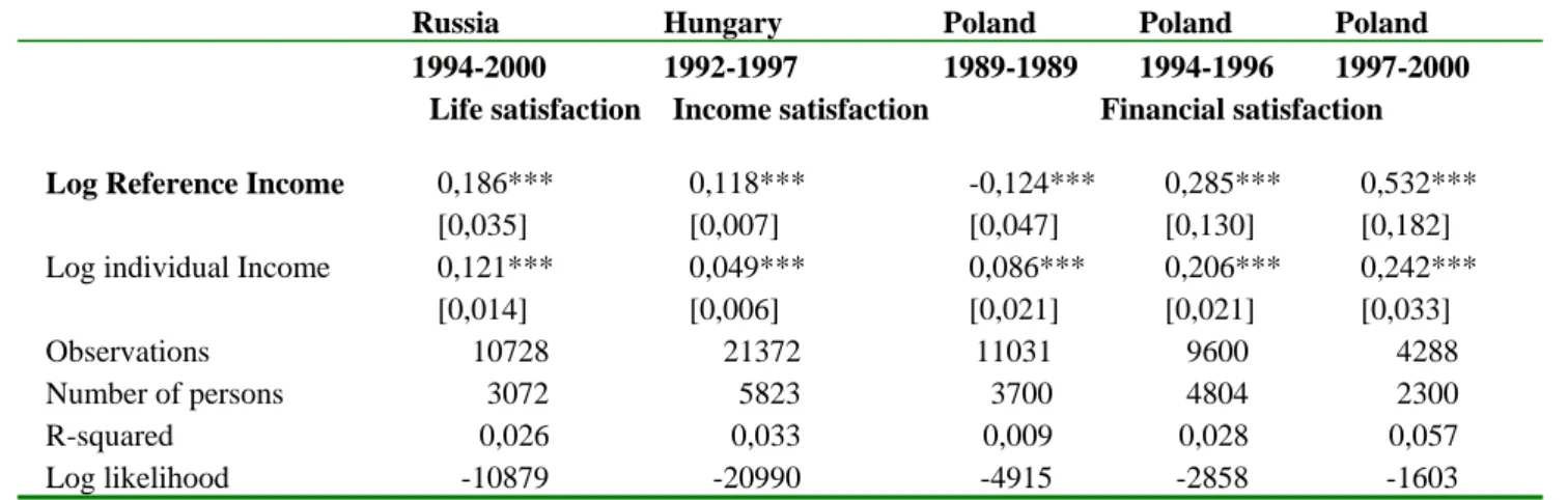
Table 1 and 2 show the positive influence of Reference Income on individual satisfaction in Post-Transition countries, using fixed effects OLS models when panel data are available (Table 1, Russia, Poland and Hungary) and simple OLS models when only cross-section data are available (Table 2, Baltic countries).
For simplicity, tables only display the regressions of Income Satisfaction. However, the results hold for other categories of subjective satisfaction. In Hungary for instance, reference income exerts a positive influence on satisfaction with future perspectives, with life, and with standard of living; it also improves financial expectations. In Baltic countries as well, reference income exerts a positive influence on satisfaction with economic situation over the past 12 months, on expectations of improvement in the household’s economic situation over the next 12 months; and even on the tolerance of inequality.
A spectacular result is obtained with Polish data (Table 1). Up to 1990, Poland was still a Socialist regime (notwithstanding partial reforms), hence a regime with extremely little change and uncertainty in terms of occupations and income. Transition began abruptly in January 1990, with the so-called “shock therapy” involving inter alia the overnight liberalization of prices and transactions. This triggered a dynamic process of change in the income distribution and
individual prospects (Sachs, 1993). As an illustration, I calculated an index of mobility defined as the average square number of deciles change across years (see Atkinson et al., 1992, for a discussion of this indicator). The order of magnitude of this index rises from about 2 before 1990, to about 4.5 afterwards (Senik, 2005b, Table A.XI). In order to take this sharp evolution into account, I leave year 1990 aside and run the regressions on the three separate sub-periods. I obtain a negative sign for the coefficient of reference income with the panel 1987-1989, and a positive coefficient for the two subsequent panels (Table 1). I interpret this contrast between the sub-periods of the Polish panel as a powerful illustration of the fact that reference income becomes valuable information when instability rises.
By contrast, Table 3 shows that in stable European countries, the sign of Reference Income is predominantly negative, with the exception of Ireland and Spain where it is significantly positive. These results, which confirm those of Clark and Oswald (1996) and Ferrer-i-Carbonnell (2004), suggest that comparison effects most often dominate information effects in the “old Europe”. As a complement to this result, I have used French data for which I have more subjective variables, from a separate French source (INSEE): I find that not only does financial satisfaction decrease with reference income, but also do other subjective variables, such as the probability of declaring that one’s “situation has improved compared to last year”, and that “household resources are sufficient to live on” (See Senik, 2005b, for the corresponding tables). This comparison effect is attenuated for individuals in the upper part of the reference group: comparisons are more effective upwards. A similar asymmetry was uncovered by Ferrer-i-Carbonnell (2004) with German data.
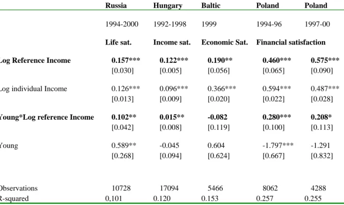
value should be higher for younger people, whose future perspectives are longer. This is confirmed by Table 4 who shows that indeed, in most cases, the positive impact of reference income is higher for people under the age of 41. The positive impact of reference income is also higher for individuals who experience particularly high income volatility over time, i.e. those whose standard deviation of real individual income across rounds is superior to the national mean standard deviation (Table 5).
Finally, the Russian survey allows verifying that Reference Income is used as an information category, using the subjective Expectations question: “Do you think that in the next 12 months
you and your family will live better than today or worse? (much worse/ worse/…/much better”, 5 modalities). I verify that this proxy for expectations is indeed influenced by Reference Income,
and that, in turn, it influences satisfaction: I run a two-stages least squares regression of standardized Life Satisfaction on Expectations instrumented by Reference Income. In the first stage regression of Expectations, the coefficient on Reference Income is 0,0326 with a standard deviation of 0,008; in the second stage regression of standardized Life Satisfaction, the coefficient on instrumented Expectations is 3,76 with a standard deviation of 1,12. Hence, Reference Income does seem to influence Life Satisfaction via Expectations. I refer the interested reader to a companion paper dedicated to the role of expectations, which develops this point with more details (Senik, 2006).
As an additional verification5, I use the first round of the European Social Survey (ESS, 2003)
that covers 21 European countries, including four “Eastern” formerly Socialist countries. The ESS is not panel and there are not many observations for each country, so I build the Reference Income as the average labour income by country*occupation (ISCO 1 digit level); there are not
enough observations per country to build more precise categories. I then regress happiness on Reference Income controlling for age, age square, gender, household income, household size, employment status, education and country dummies. Of course, this is a very crude test, but it turns out that Reference Income is only positive and significant for the former Transition countries: the Czech republic, Hungary, Poland, Slovenia (and Israel - curiously)6; in other
countries of the “old Europe” the coefficient is not significant! A possible interpretation is that this average professional income is relevant enough as a source of information in Eastern countries, but is not precise enough to play the role of a comparison benchmark in West European countries.
In summary, the data from post-Transition countries support the interpretation of Reference Income as a source of information: younger people and those more exposed to uncertainty give a higher value to the information conveyed by the income of their professional peers. Hence, the difference between Eastern and Western Europe seems to pertain to the higher volatility and uncertainty that Easterners are confronted with. The experience of Poland, i.e. the fact that the sign of the coefficient on Reference Income changes with the beginning of the Transition strengthens this interpretation.
I now turn to the American environment, which is not as volatile as that of Eastern Europe, but where income mobility is considered to be higher than in Western Europe.
III.2. Hirschman in America
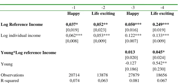
A surprising result is that, in the United-States, happiness and the feeling that “life is exciting” rather than “life is dull” (two possible answers to the satisfaction question in the GSS survey)
increase with the income of one’s professional peers (Table 6). For space constraints, I present the result of the regression on the pooled data (1972-2001) including year dummies, but I have checked that the result holds in year by year regressions. Column 4 shows that the effect of Reference Income is reinforced for the young (under 41 years old).
If the interpretation of this Europe/USA divide lies in the difference in social mobility, then the positive effect of Reference Income should be reinforced for those whose perception of mobility is higher. Indeed, I find that when respondents declare that their living standard is higher than that of their parents, the effect of Reference Income on the feeling that “life is exciting” is stronger (column 2 in Table 7). The positive welfare effect of Reference Income is also greater for American respondents who believe that they “have the opportunity to advance” (column 5). Symmetrically, for those who have experienced downward social mobility, the effect of Reference Income is weaker (column 4).
These observations somehow differ from that of Luttmer (2005) who provides empirical evidence of relative deprivation effects in the United States. However, Luttmer looks at the welfare effect of the average earnings of one’s neighbors (and shows that it is negative): it is clear that the informational content of this income category differs from that of one’s professional group.
III.3. Ruling out the measurement error interpretation
A standard worry about the estimates of the coefficient on reference income is that it is biased upwards because it serves as a proxy for true own income when the own income variable is measured with error. Thus a more prosaic interpretation of the results is that in the New Europe
and the GSS data, the Income variable is measured with relatively a lot of errors compared to income measures in the Western European Surveys (although there is nothing about the databases that inclines me to adhere to this view). I present three arguments that help resisting this interpretation.
The first two arguments are based on the recourse to consumption variables, under the assumption that measurement error in consumption and income are uncorrelated (cf. Ravallion and Lokshin, 2000). First, simply introducing household expenditure in the regression of satisfaction, together with own income and reference income, should correct part of the measurement error of own income. Accordingly, whenever available, I have included this variable in the list of the controls of the regressions.
Second, I instrument Own Income using Household Consumption and I verify that the coefficient on Reference Income remains positive (as well as that on Own Income). The data (here RLMS) pass this test: both instrumented log Own Income and log Reference Income are significantly positive in the regression of Life Satisfaction7.
Third, in a previous version of this paper, I was running the regressions of Life Satisfaction on Reference Income and Residual Income (Yit - Ŷ it), instead of Reference Income (Ŷ it) and Own Income (Yit). If measurement errors were driving the results, one would expect the magnitude of the coefficient on Residual Income to be lower when the coefficient of Reference Income is higher. It is obvious from the tables in Senik (2005b) that this prediction is not verified8
The positive influence of Reference Income on Life Satisfaction thus seems to be a robust result, which can hardly be attributed to measurement errors in own income.
This set of results suggests that in post-Transition countries and in the United-States, the typical income of one’s professional peers is used as a source of information rather than as a benchmark for comparison. By contrast, in Western Europe, comparison effects are dominant. This certainly has to do with differences in the perceived economic environment. Americans and East-Europeans9 perceive a higher degree of mobility (and uncertainty for the latter), which gives a
higher value to information. Of course mobility is not equivalent to uncertainty; however, both can have the effect of neutralizing the aversion of people to income differences, by emphasizing the informational content of the income distribution.
These different attitudes towards relative income are associated with a different tolerance to income inequality across the former iron curtain. An illustration is given by the tax structure in Europe. In average, the marginal top personal income tax rate is almost 14 points higher in Western Europe10 as it is in Post-Transition countries (see Senik, 2005b, Table A.XII). Taxes on
profits are also much lower in Post-Transition countries. A wave of low and flat tax rates has recently spread over Eastern countries - coinciding with a period of dramatic rise in income inequality (see Senik, 2005b, Table A.XIII). The interpretation offered by the paper is that this low demand for income equalization is typical of the period of transformation that the “new Europe” is experiencing, and during which informational effects are predominant. This might shed some light on the Kuznet’s curve, suggesting that one of the reasons why income inequality grows during the early stage of development is because agents have a lower aversion for it, hence do not elicit redistributive tax policies.
IV. CONCLUSIONS
Using mostly panel data, with over one million observations, this paper shows that the average income in one’s professional group affects individual subjective well-being negatively in “old” European countries, whereas the correlation is positive in post-Transition economies. In Poland, the relative importance of these effects is reversed with the beginning of Transition: comparison effects dominate until 1989 whereas information effects are predominant from 1990 onwards. It is remarkable that Americans react positively to a rise in their professional reference income, which makes them closer to East-Europeans than to West-Europeans.
Together with the evidence brought by Alesina et al. (2004), Alesina and La Ferrara (2005) and Alesina and Angeletos (2005), this suggests that the attitude towards income distribution divides New European countries and the United States on one side, and the “old Europe” on the other side. At a time of ongoing European enlargement, uncovering this divergence in preferences is of interest. Of course, this gap could vanish when the mobility and uncertainty that characterize countries of the New Europe decrease. Can a society keep a high degree of mobility for a long period? Whether this is actually the case of the United-States is still an open and debated question, even though such seems to be the belief of the inhabitants.
Beyond these national differences, one general lesson of this paper is the importance of income non-market interactions. Another lesson is that GDP growth remains an objective and an indicator of welfare, especially in Transition countries. With respect to this issue, this paper shows that my welfare not only improves with my own income, but that it sometimes also increases with the growth of other people’s income.
REFERENCES
Alesina A., and Angeletos G-M., 2005, “Fairness and Redistribution: US versus Europe”,
American Economic Review, 95: 913-35.
Alesina A., and la Ferrara E., 2005, “Preferences for Redistribution in the Land of Opportunities”, Journal of Public Economics, 89: 897-931.
Alesina A., di Tella R. and MacCulloch R., 2004, “Inequality and Happiness: are Europeans and Americans Different?”, Journal of Public Economics, 88 (9-10), 2009-2042.
Alesina A., Glaeser E. and Sacerdote B., 2001, « Why Doesn’t the US Have a European-Style Welfare System ? », Brookings Papers on Economic Activity, Fall, 187-278.
Atkinson T., Bourguignon F. and Morrisson C., 1992, Empirical Studies in Earnings Mobility, Harwood Academic Publishers.
Benabou R. and E. Ok, 2001, “Social Mobility and the Demand for Redistribution: the POUM Hypothesis”, The Quarterly Journal of Economics, May.
Blanchflower D. and Oswald A., 2004, “Well-Being over Time in Britain and the USA”,
Journal of Public Economics, 88: 1359-1386.
Caplin A. and Leahy J., 2001, “Psychological Expected Utility and Anticipatory Feelings”, The
Quarterly Journal of Economics, CXVI, (1), 55-80.
Clark A. and Oswald A., 1996, “Satisfaction and Comparison Income”, Journal of Public
Economics, 61, 359-381.
Cooper B., Garcia-Penalosa C. and Funk P., 2001, “Status Effects and Negative Utility Growth”,
The Economic Journal, 111, 642-655.
Corneo G. and Grüner H-P., 2000, “Social Limits to Redistribution”, American Economic
Review, 90, 1491-1507.
Daveri F., and Silva O., 2004, “Not only Nokia: what Finland Tells us about New Economic Growth”, Economic Policy, April, 117-163.
Di Tella, MacCulloch and Owald, 2003, “The Macroeconomics of Happiness”, Review of
Economics and Statistics, 85(4), 809-827.
Di Tella, Rafael and MacCulloch, Robert, 2006, “Some Uses of Happiness Data in Economics”, The Journal of Economic Perspectives, Volume 20, Number 1, Winter 2006, pp. 25-46(22). Easterlin R., 1995, “Will Raising the Incomes of All Improve the Happiness of All ?”, Journal
of Economic Behaviour and Organizations, 27, 35-47.
European Community Household Panel:
http://forum.europa.eu.int/irc/dsis/echpanel/info/data/information.html. European Social Survey: http://www.europeansocialsurvey.org.
Ferrer-i-Carbonnell A. and Frijters P., 2004, « How Important is Methodology for the Estimates of the Determinants of Happiness ? », Economic Journal, 114: 641:659.
Ferrer-i-Carbonnell A., 2004, “Income and Well-Being; an Empirical Analysis of the Comparison Income Effect”, Journal of Public Economics, 88.
Frank R., 1997, “The Frame of Reference as a Public Good”, Economic Journal, 107, 1832-47. Frey B. and Benz M., 2003, “Being Independent Is a Great Thing: Subjective Evaluations of
Self-Employment and Hierarchy”. Institute for Empirical Research in Economics Working Paper No. 135.
Frey B. and Stutzer A., 2002a, Happiness and Economics, Princeton University Press.
Frey B. and Stutzer A., 2002b, « What Can Economists Learn from Happiness Research ? »,
Journal of Economic Literature, XL(2), 402-35.
Frijters P., Haisken-DeNew P., Shields M., 2004, « Money Does Matter! Evidence from Increasing Real Income and Life Satisfaction in East Germany Following Reunification »,
The American Economic Review, 94(3) 730-740.
Hirschman A., with Rothschild M., 1973, “The Changing Tolerance for Income Inequality in the Course of Economic Development”, Quarterly Journal of Economics, LXXXVII(4), 544-566.
Kahneman D., Krueger A.B., Schkade D., Schwarz N., Stone A., 2004, “Toward National Well-Being Accounts”, The American Economic Review, 94(2), 429-434.
Lungqvist and Uhlig, 2000, “Tax Policy and Aggregate Demand under Catching Up with the Jones”, American Economic Review, 90, 356-366.
Luttmer E., 2002, “Measuring Economic Mobility and Inequality: Disentangling Real Events from Noisy Data”, Harris School of Public Policy Studies, University of Chicago, mimeo. Luttmer E., 2005, “Neighbors as Negatives: Relative Earnings and Well-Being”, Quarterly
Journal of Economics, 120: 963:1002.
Manski C. and Straub J., 2000, « Economic Analysis of Social Interactions », Journal of
Economic Perspectives, 14(3), 115-136.
Journal of Economic Behavior and Organization, 45, 251-278.
NORBALT Baltic surveys: http://www.fafo.no/norbalt.
Piketty T., 1995, “Social Mobility and Redistributive Policics”, Quarterly Journal of
Economics, CX, 551-583.
Ravallion M. and Lokshin M., 2000, “Who Wants to Redistribute ? The Tunnel Effect in 1990’s Russia”, Journal of Public Economic, 76, 87-104.
Ravallion M. and Lokshin M., 2001, “Identifying Welfare Effects from Subjective Questions”,
Economica, 68, 335-357.
Russian Longitudinal Monitoring Survey: http://www.epc.unc.edu/projects/rlms Sachs J., 1993, Poland’s Jump to the Market Economy, MIT Press.
Senik C., 2004a, "When Information Dominates Comparison. Learning from Russian Subjective Panel Data ”, Journal of Public Economics, 88(9-10), 2099-2133.
Senik C., 2005a, “What Can we Learn from Subjective Data ? The Case of Income and Well-Being”, Journal of Economic Surveys, 19(1).
Senik C., 2005b, « Ambition and Jealousy. Income Interactions in the “Old Europe” versus the “New Europe” and the United States”, PSE Working Paper n°2005-14 and IZA Discussion
Paper No. 2083.
Senik C., 2006 “Is Man Doomed to Progress? Expectations, Adaptation and Well-Being”, PSE
Working Paper n°2006-12 and IZA DP No. 2237. TARKI Hungarian survey : www.tarki.hu.
van de Stadt H., Kapteyn A. and van de Geer S., 1985, “The Relativity of Utility: Evidence from Panel Data», The Review of Economics and Statistics, 67(2), 179-187.
Van Praag, B.M.S. and Ferrer-i-Carbonell, A. (2004). Happiness Quantified: A Satisfaction.
Calculus Approach. Oxford University Press, Oxford: UK.
Van Praag, B.M.S. and Kapteyn, A. (1973). Further evidence on the individual welfare Function of income: An empirical investigation in the Netherlands. European Economic Review, vol. 4,pp.33-62.
ACKNOWLEDGEMENTS
I thank Andrew Clark, Christina Fong, Marc Gurgand, Andrew Oswald and two anonymous referees for useful suggestions, as well as participants in the Seminaire Roy, in the Paris-Jourdan workshop on “Utility and Inequality”, in the GREMAQ seminar, and in the JMA and ESPE conferences. This research has benefited from the support of a grant from CNRS (ATIP), the MIRe-DREES, funds from the 5th PCRD of the European Union (HPSE-CT-2002-00149) and financial support from the CEPREMAP. I thank Christophe Starzec for the Polish data, Mihails Hazans for the Baltic data, and the Banque de Données Socio-Politiques in France for the General
Social Survey series. The usual disclaimer applies
ENDNOTES
1 The same reasoning can be held concerning the effect of income inequality in general: the prospect for
upward mobility can dominate the aversion for inequality, depending on the degree of mobility expected by individuals (e.g. Benabou and Ok, 2001, Piketty, 1995).
2 The regressions are run for each year of each country, so there is no need to cluster, except at the
household level when many individuals inside the same household can be interviewed. Regressions are simple OLS. All specifications are based on individual income, which is essentially labor income. The specifications used for the first stage estimation of reference income are the following:
ECHP countries: log (personal income in PPP or personal wage in PPP) is regressed on gender, age, age square, education, industry, occupation, fulltime/part time, status (employee/independent/ etc.), tenure.
GSS (United States): log (linearized real personal income) is regressed on age, age square occupation, industry, education, region, nationality, gender.
Hungary (TARKI) : log (real individual income) is regressed on age, age square, gender, diploma, employment status, industry, foreigner (vs national). Cluster at the household level.
Poland 1987-1989 : log (real individual income) is regressed on age, age square, gender, diploma, employment status, occupation, region.
Poland 1994-1996: log (real individual income) is regressed on age, age square, gender, diploma, employment status, occupation.
Poland 1997-2000: log (real individual income) is regressed on age, age square, gender, diploma, employment status, occupation, industry.
Russia: log (real individual income) is regressed on age, age square, gender, occupation, employment status, industry, region, tenure. Cluster at the household level.
Baltic countries: log (real individual income) is regressed on age, age square, gender, education, occupation, employment status, industry, region, nationality, part-time/full time.
3 I am grateful to an anonymous referee for these suggestions.
4 In principle, the survey itself is harmonized in the sense that the same questions, with the same response
categories, are asked of households in the various countries. Some countries withdrew from the project after a number of years. This is the case of the United Kingdom, for which there are only 3 years of true ECHP data (1994-1996). To make up for this defection, the ECHP data includes the national British Household Panel Survey for the years 1995-2001. Some years are missing for other countries as well: data from Germany and Luxembourg are only available for the years 1994-1996; 1994 is missing for Austria; and 1994 and 1995 are missing for Finland.
5 I am grateful to an anonymous referee for this suggestion.
6 The coefficients on the log Average Group Income are: 0.885***[0.364) for the Czech republic,
0.7***[0.217] for Hungary, 0.546***[0.251] for Poland and 0.783***[0.238] for Israel. The coefficients of the other countries are not significant. Average Group Income is constructed as the average labour income by country*occupation (ISCO 1 digit). Controls include age, age square, gender, household size,
marital status, children, native, education, log household income, occupation and country dummies. Standard errors were clustered by country. The satisfaction variable was standardized.
7 I run a fixed-effects Two Stages Least Square regression of Life Satisfaction. In the first-stage
regression of log Own Income, the coefficient of log Household Expenditure is 0.174*** [0.0104]; in the second-stage fixed-effects IV regression of life Satisfaction, the coefficient of log Own Income is 0.889*** [0.095] and that of log Reference Income 0.275*** [0.071]. The number of observations was 13239 with 3420 groups. Other controls were age, age square, household size, marital status, children and education level. The entire regression output is available on request.
8 I thank two anonymous referees for suggesting these tests.
9 Table A.XI in Senik (2005b) presents the average square number of deciles change experienced by
individuals over two years. It is remarkable that the order of magnitude of this indicator is much higher in transition countries than in European countries. Based on real individual income, the average mobility indicator is about 11 in Russia, 7 in Hungary, and 5 in post-reform Poland, as against 2-3 in ECHP countries. (Note, however, that income mobility and inequality in transition countries are certainly somewhat overstated by measurement errors, as argued by Luttmer, 2002).
10 Of course, countries of the “old Europe” itself are not perfectly identical in terms of preference for
income redistribution. However, even the most liberal of them have higher taxes than do Transition countries.
Table 1. Satisfaction and Reference Income in Eastern Europe Fixed-Effects OLS estimates of Standardized Satisfaction
Russia Hungary Poland Poland Poland
1994-2000 1992-1997 1989-1989 1994-1996 1997-2000 Life satisfaction Income satisfaction Financial satisfaction
Log Reference Income 0,186*** 0,118*** -0,124*** 0,285*** 0,532***
[0,035] [0,007] [0,047] [0,130] [0,182]
Log individual Income 0,121*** 0,049*** 0,086*** 0,206*** 0,242***
[0,014] [0,006] [0,021] [0,021] [0,033]
Observations 10728 21372 11031 9600 4288
Number of persons 3072 5823 3700 4804 2300
R-squared 0,026 0,033 0,009 0,028 0,057
Log likelihood -10879 -20990 -4915 -2858 -1603
Controls: age, age square, household size, marital status, children, education, log household expenditure. Excluded: employment status, industry, occupation, region.
Russia, Life satisfaction: To what extent are you satisfied with your life in general at the present time ? Very satisfied …
not at all satisfied » (5 modalities).
Hungary, Income satisfaction: « Please tell me on a scale from 1 to 10 how satisfied you are with your income ?». Poland, Financial satisfaction : «How do you evaluate your financial situation: “1.very good, 2.good, 3.normal, 4.bad,
5.very bad”.
Reference income is calculated on the basis of individual monthly wage. Standardized Satisfaction variables.
Bootstrapped standard deviation of log Reference Income (1000 replications).
Table 2. Satisfaction and Reference Income in Baltic countries OLS Estimates of Standardized Satisfaction
All Baltic Estonia Latvia Lithuania
Economic Satisfaction, 1999
Log Reference Income 0,184*** 0,364*** 0,166** 0,207**
[0,048] [0,065] [0,073] [0,096]
Log individual income 0,363*** 0,344*** 0,350*** 0,459***
[0,024] [0,026] [0,031] [0,044]
Observations 5466 2666 1588 1215
R-squared 0,157 0,158 0,133 0,138
Controls: age, age square, gender, household size, marital status, children, native, education, log household expenditure, country dummies in column 1.
Excluded: employment status, industry, occupation, region and part-time/full-time. Cluster (country) column one.
Economic Satisfaction : « Considering the total situation of your household, please tell me which of the following statements best describes your situation : we are among the well-offs … we are poor » (5 modalities). Reference income is calculated on the basis of individual monthly wage.
Standardized Satisfaction variables.
Table 3. Satisfaction and Reference Income in Stable Europe (ECHP 1994-2000)
Fixed Effects OLS Estimates of Standardized Satisfaction
« Could you indicate on a scale from 1 to 6 your degree of satisfaction of your financial situation? »
UK BHPS Germany Denmark Netherlands Belgium Luxembourg France UK ECHP Ireland Italy Greece Spain Portugal Austria Finland -0,011*** 0,027*** -0,004* 0,010*** -0,006*** -0,063*** 0,008 -0,018*** 0,026*** 0,005 -0,002 0,025*** 0,005 -0,013** -0,041*** Log Reference Income by wave and country [0,002] [0,009] [0,002] [0,002] [0,002] [0,022] [0,005] [0,006] [0,007] [0,004] [0,007] [0,005] [0,005] [0,006] [0,002] 0,042*** 0,054*** 0,055*** 0,069*** 0,035*** 0,144*** 0,077*** 0,047*** 0,015** 0,009** 0,019*** 0,020*** 0,038*** 0,108*** 0,064*** Log monthly wage
[0,005] [0,009] [0,007] [0,006] [0,006] [0,021] [0,006] [0,007] [0,007] [0,004] [0,006] [0,005] [0,005] [0,008] [0,005] Observations 40845 15034 22900 42000 21077 2986 42174 12087 21124 50700 30697 42257 43945 23046 21929 Nb individuals 8697 6147 5257 9818 4707 1186 9436 6081 6460 11456 7594 11401 9587 5666 6504 R-squared 0,05 0,055 0,084 0,066 0,051 0,163 0,054 0,055 0,046 0,051 0,11 0,061 0,065 0,066 0,069 log likelihood -54732 -19756 -29179 -54267 -26378 -3811 -55311 -15533 -27869 -67847 -41543 -57301 -58450 -30202 -28838
Controls: age, age square, household size, marital status, children, education. Excluded: employment status, industry, occupation, part-time/full-time, tenure. Reference income is calculated on the basis of individual monthly wage. Standardized Satisfaction variables.
Table 4. The Higher Effect of Reference Income for Younger People in Eastern Europe OLS estimates of Standardized Satisfaction
Russia Hungary Baltic Poland Poland
1994-2000 1992-1998 1999 1994-96 1997-00
Life sat. Income sat. Economic Sat. Financial satisfaction
Log Reference Income 0.157*** 0.122*** 0.190** 0.460*** 0.575*** [0.030] [0.005] [0.056] [0.065] [0.090]
Log individual Income 0.126*** 0.096*** 0.366*** 0.594*** 0.487***
[0.013] [0.009] [0.020] [0.022] [0.028] Young*Log reference Income 0.102** 0.015** -0.082 0.280*** 0.208*
[0.042] [0.008] [0.119] [0.100] [0.113]
Young 0.589** -0.045 0.604 -1.797*** -1.291
[0.268] [0.094] [0.624] [0.667] [0.832]
Observations 10728 17094 5466 8062 4288
R-squared 0,101 0.120 0.153 0.257 0.255
Controls: age, age square, gender, household size, marital status, children, native, education, log household expenditure, country dummies for Baltic countries, year dummies for the others.
Excluded: employment status, industry, occupation, region and part-time/full-time for Baltic countries. Reference income is calculated on the basis of individual monthly wage.
Young is defined as less than 41 years. Standard errors clustered by individual. Standardized Satisfaction variables.
Bootstrapped standard deviation of log Reference Income (1000 replications).
Russia, Life satisfaction: To what extent are you satisfied with your life in general at the present time ? Very
satisfied … not at all satisfied » (5 modalities).
Hungary, Income satisfaction: « Please tell me on a scale from 1 to 10 how satisfied you are with your
income ?».
Baltic, Economic satisfaction : « Considering the total situation of your household, please tell me which of the following statements best describes your situation : we are among the well-offs … we are poor » (5 modalities). Poland, Financial satisfaction : «How do you evaluate your financial situation: “1.very good, 2.good, 3.normal,
Table 5. The Higher Effect of Reference Income in Presence of High Volatility OLS Estimates of Standardized Life Satisfaction
-1 -2 -3 -4
Russia 2000 Hungary 1996 Poland 1996 Poland 2000 Life satisfaction Income satisfaction Financial satisfaction
Log Reference Income 0,312*** 0.157*** 0.989*** 0.767***
[0,084] [0.021] [0.116] [0.117]
Log individual Income 0,023 0.063* 0.352*** 0.418***
[0,038] [0.036] [0.047] [0.046] -0,026 0.017** 0.212*** 0.018** High Volatility*log Reference Income [0,111] [0.007] [0.042] [0.007] Observations 960 822 2666 1763 R-squared 0,096 0.212 0.258 0.228
Sub-sample of men. Regression on the last year of the panel.
Controls: age, age square, gender, household size, marital status, children, native, education, log household expenditure, year dummies, volatility.
Excluded: employment status, industry, occupation, region.
Reference income is calculated on the basis of individual monthly wage.
Volatility is measured as the standard deviation of individual income across all years of the panel. High volatility is defined as above average.
Standard errors clustered by individual. Standardized Satisfaction variables.
Bootstrapped standard deviation of log Reference Income (1000 replications).
Russia, Life satisfaction: To what extent are you satisfied with your life in general at the present time ? Very
satisfied … not at all satisfied » (5 modalities).
Hungary, Income satisfaction: « Please tell me on a scale from 1 to 10 how satisfied you are with your
income ?».
Poland, Financial satisfaction : «How do you evaluate your financial situation: “1.very good, 2.good,
APPENDIX.
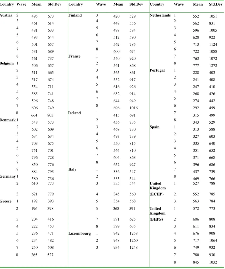
Table A.I ECHP Individual Monthly Wages in PPP
Country Wave Mean Std.Dev Country Wave Mean Std.Dev Country Wave Mean Std.Dev
Austria 2 495 673 Finland 3 420 529 Netherlands 1 552 1051
3 461 614 4 448 556 2 562 831 4 481 633 5 497 584 3 596 1005 5 493 644 6 512 590 4 628 922 6 501 657 7 562 785 5 713 1124 7 531 689 8 600 674 6 722 1088 8 561 737 France 1 540 920 7 763 1072 Belgium 1 506 657 2 561 868 8 777 1272 2 511 665 3 565 861 Portugal 1 228 403 3 517 674 4 552 917 2 241 408 4 554 711 5 616 926 3 247 410 5 585 741 6 632 914 4 268 426 6 596 748 7 644 949 5 274 442 7 606 749 8 696 1016 6 292 459 8 664 803 Ireland 1 415 691 7 315 499 Denmark 1 548 573 2 456 735 8 343 529 2 602 609 3 468 730 Spain 1 313 588 3 634 634 4 497 739 2 327 603 4 703 675 5 550 815 3 335 640 5 751 701 6 564 810 4 351 652 6 796 728 7 604 863 5 371 668 7 850 776 8 652 927 6 396 686 8 884 793 Italy 1 336 547 7 437 739 Germany 1 580 736 2 335 544 8 469 766 2 610 773 3 335 544 United Kingdom 1 527 788 3 621 779 4 345 560 (ECHP) 2 552 785 Greece 1 192 393 5 354 568 3 563 784 2 196 398 6 368 591 United Kingdom 1 572 773 3 204 416 7 391 625 (BHPS) 2 606 808 4 222 453 8 399 635 3 611 834 5 236 471 Luxembourg 1 942 1258 4 676 908 6 234 482 2 948 1260 5 717 1064 7 250 508 3 934 1248 6 749 932 8 265 527 7 780 930 8 845 1032
Table A.II ECHP. Satisfaction with Financial Situation: “Could you indicate on a
scale from 1 to 6 your degree of satisfaction for your financial situation?”
1 2 3 4 5 6 7 8 9 10 11 12 13 14 57
(%) Germany Denmark Netherlands Belgium Luxembourg France UK
ECHP Ireland Italy Greece Spain Portugal Austria Finland UK BHPS Not satisfied 7 3 2 6 7 7 13 7 10 7 9 8 6 3 2 2 10 5 4 7 7 8 12 9 18 23 17 18 9 7 4 3 19 12 9 17 14 22 20 18 29 35 26 35 13 16 22 4 27 25 23 29 21 32 26 28 28 27 26 34 25 31 40 5 27 35 44 28 34 28 17 22 13 8 19 5 30 32 32 Fully satisfied 10 21 19 13 17 2 11 15 2 1 4 1 16 10 Total 100 100 100 100 100 100 100 100 100 100 100 100 100 100 100 Freq 9464 3759 8599 4205 2035 10025 10327 3403 13343 9212 11658 10891 5598 5064 8360 Based on wave 8 (2001) unless not available, in which case based on wave 1 (1994): Germany (1), Luxembourg (5), UK ECHP (7).
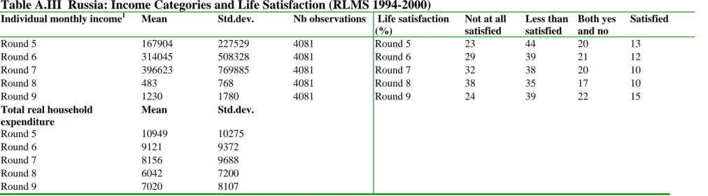
Table A.III Russia: Income Categories and Life Satisfaction (RLMS 1994-2000)
Individual monthly income1 Mean Std.dev. Nb observations Life satisfaction
(%) Not at all satisfied Less than satisfied Both yes and no Satisfied Round 5 167904 227529 4081 Round 5 23 44 20 13 Round 6 314045 508328 4081 Round 6 29 39 21 12 Round 7 396623 769885 4081 Round 7 32 38 20 10 Round 8 483 768 4081 Round 8 38 35 17 10 Round 9 1230 1780 4081 Round 9 24 39 22 15
Total real household expenditure Mean Std.dev. Round 5 10949 10275 Round 6 9121 9372 Round 7 8156 9688 Round 8 6042 7200 Round 9 7020 8107 Source : RLMS 1
In 1998 (round 8), a monetary reform divided all prices by 1000.
Table A.IV Hungary Satisfaction Categories, in % (TARKI Database)
Satisfaction with income 1992 1993 1994 1995 1996 1997
In %
Not satisfied at all 18 15 11 11 11 11
1 9 9 8 9 9 11 2 11 12 12 14 15 18 3 11 13 13 16 16 16 4 8 10 10 11 11 12 5 19 20 20 20 19 16 6 7 8 9 7 8 7 7 6 6 7 5 6 5 8 6 5 6 4 4 4 Fully satisfied 4 3 3 2 1 1 Total 100 100 100 100 100 100
Satisfaction variables: “Please tell me how satisfied you are with. your income? If you
are not at all satisfied, give 0; if you are completely satisfied, give 10.
Table A.V Hungary. Real Financial Categories in Constant Prices
Year Real household expenditure Real individual income Nb Observations
Mean SD Mean SD 1992 20948 12676 126076 339102 7265 1993 19805 11386 112117 141032 6674 1994 20175 11287 111236 179577 6220 1995 19044 10692 99458 136663 5493 1996 19633 14551 89484 119508 4807 1997 19651 10791 89325 177487 3778
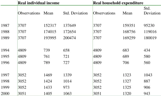
Table A.VI Poland. Real Financial Categories (Polish Household Panel, 1987-2000)
Real individual income Real household expenditure
Observations Mean Std. Deviation Observations Mean
Std. Deviation 1987 3707 152317 137649 3707 159351 95230 1988 3707 174015 172654 3707 168756 119016 1989 3707 193995 200474 3707 169259 180019 1994 4809 739 658 4809 683 434 1995 4809 761 721 4809 689 580 1996 4809 789 727 4809 706 560 1997 3052 1469 1339 3052 1323 1043 1998 3052 1424 1014 3052 1327 887 1999 3052 1433 973 3052 1325 906 2000 3051 1405 1063 3051 1320 943
Table A.VII Poland,: “How do you Evaluate your Current Financial Situation?” (Polish Household Panel, 1987-2000)
In % 1987 1988 1989 1990 1994 1995 1996 1997 1998 1999 2000 Very bad 1,1 0,6 1,2 1,5 6,8 5,5 5,0 11,4 11,2 14,1 14,6 Bad 11,9 10,7 14,3 15,4 30,5 26,9 26,6 21,7 21,7 23,0 23,2 Normal 63,2 65,4 66,2 66,3 52,8 55,8 56,5 57,1 56,7 53,0 52,9 Good 22,4 22,3 17,7 16,3 9,5 11,4 11,3 9,5 10,2 9,6 9,0 Very good 1,4 1,1 0,7 0,6 0,4 0,5 0,6 0,2 0,3 0,4 0,4
Table A.VIII Baltic Countries (NORBALT 1999 Household Survey)
Estonia Latvia Lithuania
Economic
Satisfaction (%) Estonia Latvia Lithuania
1 7 9 8 2 22 33 33 3 59 51 55 4 11 7 4 5 0 0 0 Total 100 100 100
Real individual income
in constant Euros Estonia Latvia Lithuania
mean 183 144 125
sd 178 178 120
Number observations 4532 2801 2397
Economic satisfaction: “Considering the total economic situation of your household, please tell me which of the
following statements best describes your situation: 1. we feel we are among the well-off in Estonia (Latvia, Lithuania), 2. we are not rich but we manage to live well, 3. we are neither rich nor poor, 4. we are not poor but on the verge of poverty, 5. we are poor”.
Table A.IX American General Social Survey
Real individual Income in Constant $
Life is : Respondent is :
Year Mean Std. Dev Year dull routine exciting Total In % not too happy pretty happy very happy
1972 28389 20552 In % 1972 16,5 53,2 30,3 1973 31362 22397 1973 5,1 49,4 45,5 100 1973 13,1 51,1 35,9 1974 32125 23988 1974 4,7 51,8 43,5 100 1974 13,1 49 37,9 1975 29404 22256 100 1975 13,1 54,1 32,9 1976 28274 21368 1976 3,7 51,6 44,8 100 1976 12,5 53,4 34,1 1977 32641 29325 1977 6,8 48,9 44,4 100 1977 11,9 53,2 34,8 1978 30178 25723 1978 9,6 56,1 34,3 1980 31333 27256 1980 5,6 48,4 46 100 1980 13,3 52,7 33,9 1982 24546 20668 1982 6,6 50,2 43,1 100 1982 14,5 54,9 30,6 1983 30693 29432 1983 12,8 56,1 31,2 1984 28299 24026 1984 5 48,2 46,8 100 1984 12,9 52,3 34,7 1985 30434 27736 1985 6,5 45,6 47,9 100 1985 11,4 60 28,6 1986 28539 25023 1986 11,4 56,3 32,3 1987 28110 23270 1987 4,6 51,5 44 100 1987 13,4 57,5 29,1 1988 28917 23953 1988 5 50 45,1 100 1988 9,3 56,8 34 1989 30969 24889 1989 5,3 50,2 44,5 100 1989 9,7 57,7 32,6 1990 33096 29715 1990 5 50,1 45 100 1990 9 57,6 33,4 1991 26911 21661 1991 4,2 51,5 44,3 100 1991 11 58 31,1 1993 32577 30568 1993 6,5 47,1 46,5 100 1993 11,1 57,3 31,6 1994 31136 26879 1994 4,2 48,4 47,4 100 1994 12,2 59 28,8 1996 31991 27299 1996 4,2 45,9 50 100 1996 12,1 57,5 30,4 1998 30558 26556 1998 5,5 49,4 45,1 100 1998 12,1 56,1 31,8 2000 33227 33941 2000 4,9 48,7 46,4 100 2000 10,6 57,7 31,7 2002 34930 35834 2002 3,7 44,2 52,1 100 2002 12,4 57,3 30,3 Mean 5,1 49 45,9 100 Mean 12,1 55,9 32,1