Teaching Digital and Analog Modulation to
Undergradute Information Technology Students
Using Matlab and Simulink
M. Boulmalf
1, Y. Semmar
2, A. Lakas
3, and K. Shuaib
31
School of Science & Engineering, Al Akhawayn University in Ifrane, Morocco
2College of Education, Qatar University, Doha, Qatar
3
College of Information Technology, UAE University, Al Ain, UAE
E-mail: [email protected]
Al Akhawayn University in Ifrane , Morocco, P.O. Box: 2129
Abstract—Teaching mathematical intensive engineering based
courses to undergraduate Information Technology students poses a great challenge to instructors. In this paper we provide an efficient and effective method for teaching digital and analog modulation to undergraduate students enrolled in an Information Technology program which does not require a strong foundation in mathematics as in the case of an Engineering program. The used approach utilizes Matlab packages, Simulink, and Communication Blockset to simulate analog and digital modulation techniques avoiding the derivation of any mathematics formulations and without coding. A survey that was distributed to Information Technology students who were taught using this approach showed a high level of satisfaction in understanding all modulation concepts.
Keywords: Matlab; Modulation; Simulink, Communications Blokset
I. INTRODUCTION
Matlab is a numerical computing environment and a 4th
generation programming language. It is a high level language and interactive environment that enables users to perform intensive calculations based tasks very fast. Developed by Mathworks [5], Matlab allows matrix manipulation, plotting of functions and data, implementation of algorithms, creation of user interfaces, and interfacing with programs in other languages. Matlab has been widely adopted for over 25 years in the academic community, industry and research centers. It was originally written to provide easy access to LINPACK and EISPACK software packages [1-4]. The Matlab software provides the users with a large collection of toolboxes and modules for a variety of applications in many fields of interest. Simulink [6] is an interactive graphical tool that was added to Matlab to make the modeling and simulation of various systems as easy as connecting predefined and designed building blocks. Simulink contains many block sets that are used in almost all applications such as the communication block set and the signal processing block set.
Research using Matlab/Simulink has been conducted for many years in academia, industry and also military. Many researchers have published papers using Matlab/Simuling for simulating particular systems. For examples, the authors in [7, 8, 10, 11] used Matlab/Simulink to model components and
performance of various wireless communication systems. Others have utilized Matlab/Simulink as a research tool for army and military based applications [13, 14].
Matlab has been used as a teaching aid in many subjects such as mathematics, physics, heat conduction, control systems, mechatronics, mechanical design, circuit design, communication theory, random processes, electronics and many more disciplines and applications [4, 5, 9, 12, 15, 16].
In this paper, we provide an efficient and effective method for teaching digital and analog modulation techniques to undergraduate students enrolled in an Information Technology program which does not require a strong foundation in mathematics as in the case of an Engineering program. The used approach utilizes Matlab and Similink blocksets to simulate analog and digital modulation techniques. To assess the degree to which Matlab/Simulink helped students to understand the taught concepts, a survey was distributed to students and the results were analyzed using Statistical Package for the Social Sciences (SPSS [25]) and presented in this paper.
The rest of the paper is organized as follow: In section 2, analog and digital modulation techniques are introduced. Section 3, discusses the use of Simulink and the communication toolboxes available in Matlab to study modulation techniques. Section 4 shows the results of the students’ survey, and section 5 concludes the paper.
II. ANALOG AND DIGITAL MODULATION
In general, modulation is used to give the transmitted signal properties which are best suited to the transmission channel or environment. Specifically, modulation is the process of imparting the source information onto a band pass signal with a carrier frequency, fc, by the introduction of
amplitude or phase perturbations or both. This band pass signal is called the modulated signal and the base band source signal is called the modulating signal [4]. At the receiver end a mean to translate the higher frequencies back to the audio range is implemented and this is called demodulation.
A. Amplitude modulation (AM)
Audio signals at most occupy the frequency range 0-20 KHz (minimum 15 Km wavelength). This range of frequencies is too low to transmit directly as electromagnetic radiation, particularly due to the prohibitive sizes of the transmitter and receiver antennas which would be required. Antennas must have lengths of the order of the wavelength of the EM radiation of interest. Higher frequencies permit much more effective and practical transmission; however, these lie outside the audio range. For example, AM radio broadcasting occurs at frequencies of the order of 1 MHz.
In standard AM, the audio signal is shifted in amplitude by adding a DC component and then multiplied by a sinusoid at the carrier frequency, fc. The carrier frequency is much
higher than the audio frequency band. We consider a mathematical description of amplitude modulation. Following the nomenclature of Couch’s textbook [4], let the audio message signal be m(t), where m(t) is band limited to “W” Hz, and let Ac be the message amplitude (or gain).
Let ωc = 2πfc be the carrier frequency in radians per
second where fc >> W. Then the amplitude modulated signal
s(t) can be expressed as
)
cos(
)]
(
1
[
)
(
t
A
m
t
t
s
=
c+
μ
ω
c)
cos(
)
(
)
cos(
)
(
t
A
t
A
m
t
t
s
=
cω
c+
cμ
ω
cThe constant, μ, is selected such that
1
)
(
1
<
<
−
μ
m
t
The students shall understand very well the above formulas and they have to write codes using Matlab to draw the following curves depicted in Figure 1.
Figure 1: AM modulation using Matlab code Figure 1 depicts the audio signal, the carrier, and the amplitude modulated signal. This result is a coding the above formulas of AM using Matlab codes which is not easy for the non engineering students.
B. Frequency modulation (FM)
Frequency modulation encodes the message, m(t), by making the instantaneous frequency deviation about fc
proportional to m(t). Frequency Modulation is a special case of
Angle Modulated signaling. In angle modulated signaling the
complex envelope is:
) (
)
(
j t ce
A
t
g
=
θNote that this is in polar form so we can immediately say what the amplitude modulation is R(t) and the phase modulation is
simply θ(t). The amplitude modulation is:
c
A
t
g
t
R
(
)
=
(
)
=
The phase modulation is simply θ(t) and for angle modulated signals is a linear function of the modulating signal m(t). For FM the phase is proportional to the integral of m(t):
∫
−∞=
D
f tm
d
t
σ
σ
θ
(
)
(
)
Where the frequency deviation constant Df has units of
radians per volt-second. So the frequency modulated FM signal is:
⎥⎦
⎤
⎢⎣
⎡
+
=
∫
∞ − t f c cf
t
D
m
d
A
t
s
(
)
cos
2
π
(
σ
)
σ
The bandpass signal is represented by:
⎥⎦
⎤
⎢⎣
⎡
+
=
∫
∞ − t f c cf
t
D
m
d
A
t
s
(
)
cos
2
π
(
σ
)
σ
Figure 2: FM modulationFigure 2 illustrates the Programmed FM modulation using Matlab codes.
III. ANALOG AND DIGITAL MODULATION USING SIMULINK AND COMMUNICATION TOOLBOXES
A. Simulink
Simulink, developed by The MathWorks, is a tool for modeling, simulating and analyzing multi-domain dynamic systems. Its primary interface is a graphical block diagramming tool and a customizable set of block libraries. It offers tight integration with the rest of the MATLAB environment and provides scripting capability. Simulink is widely used in control theory and digital signal processing for multi-domain simulation and design.
Simulink is integrated with MATLAB, providing immediate access to an extensive range of tools for algorithm development, data visualization, data analysis and access, and numerical computation. The Key Features of Simulink include: [6]
• Extensive and expandable libraries of predefined blocks.
• Interactive graphical editor for assembling and managing intuitive block diagrams.
• Ability to manage complex designs by segmenting models into hierarchies of design components.
• Model Explorer to navigate, create, configure, and search all signals, parameters, and properties of models. • Ability to interface with other simulation programs and incorporate hand-written code, including MATLAB algorithms.
• Option to run fixed- or variable-step simulations of time-varying systems interactively or through batch simulation.
• Functions for interactively defining inputs and viewing outputs to evaluate model behavior.
• Graphical debugger to examine simulation results and diagnose unexpected behavior in designs.
• Full access to MATLAB for analyzing and visualizing data , developing graphical user interfaces, and creating model data and parameters.
• Model analysis and diagnostics tools to ensure model consistency and identify modeling errors.
With Simulink, the user can quickly create, model, and maintain a detailed block diagram of a system using a comprehensive set of predefined blocks. Simulink provides tools for hierarchical modeling, data management, and subsystem customization, making it easy to create concise, accurate representations, regardless the system’s complexity. Details on how to create and run simulation models are out of the scope of this paper, for more information on this the reader can look at the following references [6, 17, 18].
B. Communication Toolbox
Communications Toolbox extends the MATLAB technical computing environment with functions, plots, and a graphical user interface for exploring, designing, analyzing, and simulating algorithms for the physical layer of communication systems. The toolbox helps create algorithms for commercial and defense wireless or wireline systems, such as mobile handsets and base stations, wired and wireless local area networks, and digital subscriber lines. It can also be used in research and education for communication systems engineering.
The Key Features of Communication toolbox includes [5]: • Functions for designing the physical layer of
communications links, including source coding, channel coding, interleaving, modulation, channel models, and equalization.
• Graphical plots for visualizing communications signals, such as eye diagrams and constellations.
• Graphical user interface for comparing the bit error rate of a system with a wide variety of proven analytical results.
• Galois field data type for building communications algorithms.
• New channel visualization tool to visualize and explore time-varying communications channels.
C. Simulation of analog modulation
The students don’t have to derive any more the modulation formulas. He/She has just to understand the components of the equation (e.g. AM equations) and start to implement using the Simulink. Figure 3 illustrates the blocks needed to design an AM modulator. The students have to open simulink and drag and drop in the area of work all these blocks. To visualize the modulated and modulating signals, we need to add to the simulator two scopes. Scope 1 shows the original signal before the modulation. Scope 2 shows the modulated signal, it means after the modulation process. The students can also see the modulated signal in frequency domain. They need to drag and drop the Box “BFFT”. This Box does the Fast Fourier Transform operation and illustrates the signal in Frequency domain. The students are exempted to know the derivation of FFT formula.
Figure 3: The model of AM modulator using Simulink Figure 4 shows the audio signal before modulation; it is depicted by the Scope 1.
Figure 4: The modulating signal m(t)
Figure 5 illustrates the amplitude modulated signal. This signal should be transmitted over the medium.
Figure 5: The amplitude modulated signal s(t)
The frequency domain spectrum is obtained through a buffered-FFT scope, which comprises of a Fast Fourier Transform of 128 samples which also has a buffering of 64 of them in one frame. Figure 6 depicts the modulated signal in frequency domain.
Figure 6: The spectrum of the AM signal s(t)
Table 1 below lists and describes the blocks in the Analog Passband sub-library of Modulation by double-clicking on the Analog Passband icon in the main Modulation library, or by typing commanapbnd2 at the MATLAB prompt. For more details, the readers can consult the Mathwork website.
TABLE I. TABLE 1:BLOCKS FOR ANALOG MODULATION
Block Name Purpose
DSB AM Demodulator Passband Demodulate DSB-AM-modulated data
DSB AM Modulator Passband Modulate using
double-sideband amplitude modulation DSBSC AM Demodulator Passband Demodulate DSBSC-AM-modulated data
DSBSC AM Modulator Passband Modulate using double-sideband suppressed-carrier amplitude modulation
FM Demodulator Passband Demodulate FM-modulated data
FM Modulator Passband Modulate using frequency modulation
PM Demodulator Passband Demodulate PM-modulated data
PM Modulator Passband Modulate using phase modulation
SSB AM Demodulator Passband Demodulate SSB-AM-modulated data
SSB AM Modulator Passband Modulate using
single-sideband amplitude modulation
D. Simulation of Digital modulation
Table 2 lists and describes the blocks for digital modulations. Figure 7 illustrates the model for MPSK modulations using Simulink and the Communications block set. The students can vary the parameter “M” and also the Signal to Noise Ratio (SNR) and can easily draw the BER (Bit Error Rate). Figure 8 depicts the results of BER versus the SNR. The student can simulate all type of digital modulations by choosing the adequate Blocks and they can also choose different type of channels. The blocks are respectively Data generator, Modulator, Channel model, demodulator, and the BER calculator. The students are not supposed to know the formula of Probabilities of errors. The model generates a million of bits and can calculate easily the errors.
TABLE II. BLOCKS FOR DIGITAL MODULATION
Block Name Purpose
M-DPSK Demodulator
Passband Demodulate DPSK-modulated data M-DPSK Modulator
Passband
Modulate using the M-ary differential phase shift keying method
M-PSK Demodulator Passband
Demodulate PSK-modulated data M-PSK Modulator Passband Modulate using the M-ary phase shift
keying method OQPSK Demodulator
Passband Demodulate OQPSK-modulated data OQPSK Modulator
Passband
Modulate using the offset quadrature phase shift keying method
M-FSK Demodulator Passband
Modulate using the M-ary frequency shift keying method
M-FSK Modulator Passband Modulate using the M-ary frequency shift keying method
Figure 7: The Block diagram of MPSK Modulations
Figure 8: The BER versus SNR for MPSK
Figure 8 shows, for MPSK, as the value of M increase the BER increase. So, MPSK is better in term of BER when the value of M is small.
IV. RESULTSAND DISCUSSION
A 13-item survey was administered to 57 Information Technology undergraduate students. The survey tapped students' reactions to using Matlab with Simulink for learning and understanding digital and analog modulation concepts. The convenience sample of participants responded to the survey, which was based on the following, 5-point Likert scale: 5 = Strongly Agree; 4 = Agree; 3 = Somewhat Agree; 2 = Disagree; 1 = Strongly Disagree. As can be seen from Table 3, students expressed a general consensus towards their agreement of the benefits of incorporating Matlab with Simulink in their course. Most of them, for instance, claimed that the Matlab with Simulink component was very useful for helping them understand the
TABLE III. DescriptiveSTATISTICS (N=57)
Variable Min. Max. Mean SD
Knowledge before 1 1 5 3.02 1.009 Knowledge after 2 2 5 4.14 .766 Attitude 3 2 5 3.71 .762 Understanding 4 2 5 4.04 .731 Learnmore 5 1 5 3.69 .979 Easy to use 6 11 5 3.68 1.003 Approving 7 1 5 3.50 .885 Simulation experience 8 1 5 3.55 .807 Learning experience 9 1 5 3.68 .917 Interact 10 2 5 3.81 .693 Educational 11 2 5 3.89 .673 Comfortable 12 2 5 3.86 .718 Satisfied 13 2 5 3.74 .813 theoretical aspect of the course, thereby increasing their knowledge base of the subject matter.
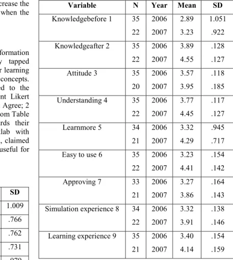
Independent Samples T-Tests were run to investigate differences between the 2006 and 2007 cohorts in terms of how they perceive the usefulness of Matlab with Sumilink. As can be seen in Table 4, higher means were observed for the 2007 students. This group of students held more favorable views about the utility of Matlab with Sumilink in their course. For example, compared to their 2006 counterparts, the 2007 cohort felt more strongly that Matlab with Simulink was easy to use (mean = 4.41), helped them understand the course much better (mean = 4.45), and that their knowledge has now increased as a result of using Matlab with Sumilink (mean = 4.55).
TABLE IV. T-Test (N=57)
Variable N Year Mean SD
Knowledgebefore 1 35 22 2006 2007 2.89 3.23 1.051 .922 Knowledgeafter 2 35 22 2006 2007 3.89 4.55 .128 .127 Attitude 3 35 20 2006 2007 3.57 3.95 .118 .185 Understanding 4 35 22 2006 2007 3.77 4.45 .117 .127 Learnmore 5 34 21 2006 2007 3.32 4.29 .945 .717 Easy to use 6 35 22 2006 2007 3.23 4.41 .154 .142 Approving 7 33 21 2006 2007 3.27 3.86 .164 .143 Simulation experience 8 34 22 2006 2007 3.32 3.91 .138 .146 Learning experience 9 35 21 2006 2007 3.40 4.14 .154 .159
Interact 10 35 22 2006 2007 3.57 4.18 .111 .125 Educational 11 35 22 2006 2007 3.63 4.32 .101 .121 Comfortable 12 35 22 2006 2007 3.63 4.23 .117 .130 Satisfied 13 35 22 2006 2007 3.43 4.23 .131 .130
A. Internal consistency reliability
A Pearson correlation matrix of the 13 Matlab with Simulink questionnaire items was run yielding a Cronbach's alpha coefficient of .91 (α = .91). The 13-item questionnaire was then subjected to factor analysis using principal axis factoring to extract the underlying factors.
B. Factor Analysis
Data from the 13-item, Matlab with Simulink questionnaire was analyzed using principal axis factoring (SPSS 14.0) to extract the underlying factors. Principal axis factoring is preferred over the principal components analysis method, which is the default option in some statistical programs including SPSS. Since it is assumed that in principal components analysis all variability in an item ought to be used, it is advantageous to use the principal axis factoring method through which the researcher can only use the variability in an item that it shares with the other items [20]. The number of factors to be extracted was based on minimum eigenvalues of 1.0 and minimum loadings of .45 of individual items under each factor. The Kaiser-Gutman procedure, through which only factors with eigenvalues of one or greater are selected, is the most often used method to determine the number of factors [21]. The varimax rotation method produced a two-factor solution, accounting for almost 62% of the total variance (see Table 7). Varimax rotation was employed because it is a type of orthogonal rotation that mathematically ensures that the resulting factors are uncorrelated with each other [21]. This is important since in exploratory factor analysis, the researcher does not know the number and the types of factors that exist, let alone whether or not they are correlated [19].
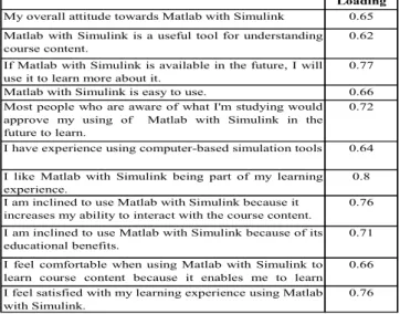
1) Factor 1: Factor 1 consisted of eleven items from the Matlab with Simulink questionnaire. The following eleven items loaded on factor 1(Table 5):
TABLE V. Eleven items from the Matlab & Simulink Questionnaire
Loading
My overall attitude towards Matlab with Simulink 0.65 Matlab with Simulink is a useful tool for understanding course content.
0.62
If Matlab with Simulink is available in the future, I will use it to learn more about it.
0.77 Matlab with Simulink is easy to use. 0.66 Most people who are aware of what I'm studying would approve my using of Matlab with Simulink in the future to learn.
0.72
I have experience using computer-based simulation tools 0.64
I like Matlab with Simulink being part of my learning experience.
0.8 I am inclined to use Matlab with Simulink because it
increases my ability to interact with the course content. 0.76
I am inclined to use Matlab with Simulink because of its educational benefits.
0.71
I feel comfortable when using Matlab with Simulink to learn course content because it enables me to learn
0.66
I feel satisfied with my learning experience using Matlab with Simulink.
0.76
2) Factor 2: Factor 2 consisted of two items from the Matlab with Simulink questionnaire. The following two items loaded on factor 2 (Table 6):
TABLE VI. Two items from the Matlab & Simulink Questionnaire
Loading
Before using Matlab with Simulink, my knowledge of course content was:
0.51 Now, my knowledge of course content is: 0.79
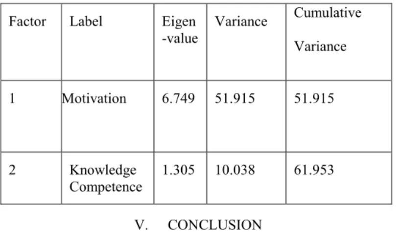
In sum, results of the factor analysis portion of this study suggested two components that characterize the School of IT students' perceptions and attitudes towards the benefits of incorporating Matlab with Simulink into the course curriculum. Factor 1 can be labeled "Motivation" since all of the items that loaded onto it are likely to contribute to learners' engagement and motivation in the classroom because of the Matlab with Simulink component. The two items that loaded on factor 2 are strictly related to students' knowledge level before and after their experience with the Matlab Simulink. Therefore, Factor 2 can be labeled as "Knowledge Competence" (See Table 8).
TABLE VII. Principal Axis Factoring (13 questionnaire items)
Factor Eigenvalue % of Variance Cumulative % 1 6.749 51.915 51.915 2 1.305 10.038 61.953
TABLE VIII. Factor Structure Factor Label Eigen
-value Variance Cumulative Variance 1 Motivation 6.749 51.915 51.915 2 Knowledge Competence 1.305 10.038 61.953 V. CONCLUSION
In this paper, the approach utilizes Matlab packages, Simulink, and Communication Blockset to simulate analog and digital modulation techniques avoiding the derivation of any mathematics formulations. A survey that was distributed to 57 Information Technology students who were taught using this approach showed a high level of satisfaction in understanding all modulation concepts. As can be seen from the survey results, students expressed a general consensus towards their agreement of the benefits of incorporating Matlab with Simulink in their course. Most of them, for instance, claimed that the Matlab with Simulink component was very useful for helping them understand the theoretical aspect of the course, thereby increasing their knowledge based on the subject matters.
REFERENCES
[1] Gilat, Amos (2004). MATLAB: An Introduction with Applications 2nd Edition. John Wiley & Sons. ISBN 978-0-471-69420-5.
[2] Quarteroni, Alfio; Fausto Saleri (2006). Scientific Computing with MATLAB and Octave. Springer. ISBN 978-3-540-32612-0.
[3] Ferreira, A.J.M. (2009). MATLAB Codes for Finite Element Analysis. Springer. ISBN 978-1-4020-9199-5. [4] Leon W. Couch, II. Digital and Analog Communication
Systems. Prentice Hall, New Jersey, sixth edition, 2001. [5] http://www.mathworks.com/access/helpdesk_r13/help/
toolbox/commblks/ref/simref-7.html#611864 [6] www.mathworks.com/products/simulink
[7] Etter, D.M. ``Engineering Problem Solving using MATLAB'' Prentice Hall, 1993.
[8] The International Journal of Engineering Education, Vol. 21, number 5, 2005.
[9] John Okyere Attia, “Teaching AC Circuit Analysis with Matlab”, the World Wide Web electronic version of the 1995 ASEE/IEEE Frontiers in Education Conference Proceedings.
[10] M. Alnuaimi, K. Shuaib and I. Jawhar, “Performance Evaluation of IEEE 802.15.4 Physical Layer Using Matlab/Simulink”, Proceeding of the IEEE IIT06 Conference, Nov19-21, 2006, Dubai, UAE.
[11] M. Boulmalf, A. Sobh, A. Shakil "Modeling and simulation of 802.11g WLAN using Matlab and Simulink," Advanced Simulation Technologies
Conference, April 18 - 22, 2004, Crystal City Arlington, Virginia.
[12] Attia, J.O, “Teaching electronics with MATLAB”, Proceeding of Frontiers in Education Conference, 1996, Salt Lake City, USA.
[13] Anderson, C. Kitts, C, “A MATLAB expert system for ground-based satellite operations”, Proceeding of the Aerospace, 2005 IEEE Conference, 5-12 March 2005, page(s): 3756 - 3762
[14] Agustina, J.V.; Peng Zhang; Kantola, R.; “Performance evaluation of GSM handover traffic in a GPRS/GSM network”, Proceeding of ISCC, 2003 Page(s):137 - 142 vol.1
[15] Bhatt, T.M.; McCain, D, “Matlab as a development environment for FPGA design”, Proceeding of Design Automation Conference, 2005. 13-17 June 2005 Page(s):607 – 610
[16] “Development of a MATLAB-Based Model for Advanced High Power Density Diesel Engine for Military
Applications” Project http://arc.engin.umich.edu/arc/research/ta4/T4DevMatlab
ModelAdvHPD.htm
[17] Mehrdad Soumekh – “Synthetic Aperture Radar Signal Processing With Matlab Algorithms”, John Wiley & Sons Inc; Apr 1, 1999.
[18] B. L. Sturm and J. Gibson, "Signals and Systems Using MATLAB: An Integrated Suite of Applications for Exploring and Teaching Media Signal Processing," in Proc. of the 2005 IEEE Frontiers in Education Conf. (FIE), Indianapolis, IN (2005).
[19] Bachiller, C. Esteban, H. Cogollos, S. San Blas, A. and Boria, V.E. “Teaching of wave propagation phenomena using MATLAB GUIs at the Universidad Politecnica of Valencia”, the IEEE Antennas and Propagation Magazine, Feb. 2003 Volume: 45, page(s): 140 – 143.
[20] www.ece.utexas.edu/~dghosh/homework/Simulink_Tutori al.pdf
[21] www.mathworks.com/academia/student_center/tutorials/i ndex.html? link=body
[22] D. Child. The essentials of factor analysis. London: Cassell, 1990.
[23] R.L. Gorsuch. Common factor anaylsis versus component analysis: Some well and little known facts. Mutivariate Behavioral Research, 25, 33-39, 1990.
[24] J.C. Loehlin. Latent variable models: An introduction to factor, path, and structural analysis (third edition). Manwah, NJ: Lawrence Erlbaum Associates, 1998.