RESEARCH OUTPUTS / RÉSULTATS DE RECHERCHE
Author(s) - Auteur(s) :
Publication date - Date de publication :
Permanent link - Permalien :
Rights / License - Licence de droit d’auteur :
Bibliothèque Universitaire Moretus Plantin
Institutional Repository - Research Portal
Dépôt Institutionnel - Portail de la Recherche
researchportal.unamur.be
University of Namur
An example of slow convergence for Newton's method on a function with globally
Lipschitz continuous Hessian
Cartis, Coralia; Gould, N. I. M.; Toint, Ph
Publication date: 2013
Document Version
Early version, also known as pre-print
Link to publication
Citation for pulished version (HARVARD):
Cartis, C, Gould, NIM & Toint, P 2013 'An example of slow convergence for Newton's method on a function with globally Lipschitz continuous Hessian' Namur center for complex systems.
General rights
Copyright and moral rights for the publications made accessible in the public portal are retained by the authors and/or other copyright owners and it is a condition of accessing publications that users recognise and abide by the legal requirements associated with these rights. • Users may download and print one copy of any publication from the public portal for the purpose of private study or research. • You may not further distribute the material or use it for any profit-making activity or commercial gain
• You may freely distribute the URL identifying the publication in the public portal ?
Take down policy
If you believe that this document breaches copyright please contact us providing details, and we will remove access to the work immediately and investigate your claim.
An example of slow convergence for Newton method on a function with globally Lipschitz continuous Hessian
by C. Cartis, N. I. M. Gould and Ph. L. Toint Report NAXYS-03-2013 3 May 2013
University of Edinburgh, Edinburgh, EH9 3JZ, Scotland (UK)
Rutherford Appleton Laboratory, Chilton, OX11 0QX, England (UK)
University of Namur, 61, rue de Bruxelles, B5000 Namur (Belgium)
http://www.fundp.ac.be/sciences/naxys
An example of slow convergence for Newton’s method on a
function with globally Lipschitz continuous Hessian
C. Cartis
∗, N. I. M. Gould
†and Ph. L. Toint
‡3 May 2013
Abstract
An example is presented where Newton’s method for unconstrained minimization is applied to find an ǫ-approximate first-order critical point of a smooth function and takes a multiple of ǫ−2 iterations and function evaluations to terminate, which is as many as the steepest-descent method in its worst-case. The novel feature of the proposed example is that the objective function has a globally Lipschitz-continuous Hessian, while a previous example published by the same authors only ensured this critical property along the path of iterates, which is impossible to verify a priori.
1
Introduction
Evaluation complexity of nonlinear optimization leads to many surprises, one of the most notable ones being that, in the worst case, steepest-descent and Newton’s method are equally slow for unconstrained optimization, thereby suggesting that the use of second-order information as implemented in the standard Newton’s method is useless in the worst-case scenario. This counter-intuitive conclusion was presented in Cartis, Gould and Toint (2010), where an example of slow convergence of Newton’s method was presented. This example shows that Newton’s method, when applied on a sufficiently smooth objective function f (x), may generate a sequence of iterates such that
k∇xf (xk)k ≥
µ 1 k + 1
¶12+η ,
where xkis the k-th iterate and η is an arbitrarily small positive number. This implies that the considered
iteration will not terminate with
k∇xf (xk)k ≤ ǫ
and ǫ ∈ (0, 1) for k < ǫ−2+τ, where τ = η/(1 + 2η). This shows that the evaluation complexity of
Newton’s method for smooth unconstrained optimization is essentially O(ǫ−2), as is known to be the
case for steepest descent (see Nesterov, 2004, pages 26-29). This example satisfies the assumption that the second derivatives of f (x) are Lipschitz continuous along the path of iterates, that is, more specifically, that
k∇xxf (xk+ t(xk+1− xk)) − ∇xxf (xk)k ≤ LHkxk+1− xkk
for all t ∈ (0, 1) and some LH ≥ 0 independent of k. The gradient of this example is globally Lipschitz
continuous.
While being formally adequate (and verified by the example if Cartis et al., 2010), this assumption has two significant drawbacks. The first is that it cannot be verified a priori, before the minimization algorithm is applied to the problem at hand. The second is that it has to be made for an infinite sequence
∗School of Mathematics, University of Edinburgh, The King’s Buildings, Edinburgh, EH9 3JZ, Scotland, UK. Email:
†Numerical Analysis Group, Rutherford Appleton Laboratory, Chilton, OX11 0QX, England (UK). Email:
‡Namur Center for Complex Systems (naXys) and Department of Mathematics, University of Namur, 61, rue de
Bru-xelles, B-5000 Namur, Belgium. Email: [email protected]
Cartis, Gould, Toint: Slow convergence of Newton’s method (draft) 2
of iterates, at least if a result is sought which is valid for all ǫ ∈ (0, 1). It is therefore desirable to verify if the stronger but simpler assumption that f (x) admits globally Lipschitz continuous second derivatives still allows the construction of an example with O(ǫ−2) evaluation complexity. It is the purpose of the
present note to discuss such an example.
2
The example
Consider the unconstrained nonlinear minimization problem given by min
x∈IRnf (x)
where f is a twice continuously differentiable function from IRn into IR, which we assume is bounded below. The standard Newton’ method for solving this problem is outlined as Algorithm 2.1, where we use the notation
gk def
= ∇xf (xk) and Hk def
= ∇xxf (xk).
Algorithm 2.1: Newton’s method for unconstrained minimization
Step 0: Initialization. A starting point x0∈ IRn is given. Compute f (x0) and g0. Set k = 0.
Step 1: Check for termination. If kgkk ≤ ǫ, terminate with xk as approximate first-order
crit-ical point.
Step 2: Step computation. Compute Hk and the step sk as the solution of the linear system
Hksk= −gk (2.1)
Step 3: Accept the next iterate. Set xk+1= xk+ sk, increment k by one and go to Step 1.
Of course, the method as described in this outline makes strong (favourable) assumptions: it assumes that the matrix Hk is positive definite for each k and also that f (xk+ sk) sufficiently reduces f (xk)
for being accepted without any specific globalization procedure, such as linesearch, trust-region or filter. However, since our example will ensure both these properties, the above description is sufficient for our purpose.
2.1
A putative iteration
Our example is two-dimensional. We therefore aim at building a function f (x, y) from IR2 into IR such that, for any ǫ ∈ (0, 1), Newton’s method essentially takes ǫ−2iterations to find an approximate first-order
critical point (xǫ, yǫ) such that
k∇(x,y)f (xǫ, yǫ)k ≤ ǫ (2.2)
when started with (x0, y0) = (0, 0).
Consider τ ∈ (0, 1) and an hypothetical sequence of iterates {(xk, yk)}∞k=0 such that gk, Hk and
fk= f (xk, yk) are defined by the relations
gk = − ³ 1 k + 1 ´12+η ³ 1 k + 1 ´2 Hk= Ã 1 0 0 ³k + 11 ´2 ! , (2.3)
Cartis, Gould, Toint: Slow convergence of Newton’s method (draft) 3 for k ≥ 0 and f0= ζ(1 + 2η) + π2 6 , fk= fk−1− 1 2 " µ 1 k + 1 ¶1+2η + µ 1 k + 1 ¶2# for k ≥ 1, (2.4) where η = η(τ )def= τ 4 − 2τ = 1 2 − τ − 1 2.
If this sequence of iterates can be generated by Newton’s method starting from the origin and applied on a twice-continuously differentiable function with globally Lipschitz continuous Hessian, then one may check that kgkk > ¯ ¯ ¯ ¯ ∂f ∂x(xk, yk) ¯ ¯ ¯ ¯ = µ 1 k + 1 ¶2−1τ > ǫ for k ≤ ǫ−2+τ,
and also that
kgkk ≤ µ 1 k + 1 ¶2−1τ + µ 1 k + 1 ¶2 ≤ 2 µ 1 k + 1 ¶2−1τ ≤ ǫ for k ≤ 4ǫ−2+τ. As a consequence, the algorithm will stop for k in a fixed multiple of ǫ−2 iterations.
2.2
A well-defined Newton scheme
The first step in our construction is to note that, since we consider Newton’s method, the step sk at
iteration k is defined by the relation (2.1), which, together with (2.3), yields that
sk = Ã s k,x sk,y ! = ³ 1 k + 1 ´12+η 1 , (2.5)
and therefore that
x0= µ 0 0 ¶ , xk= k−1 X j=0 µ 1 j + 1 ¶ 1 2+η k . (2.6)
The predicted value of the quadratic model at iteration k qk(xk+ sx, yk+ sy)
def
= fk+ hgk, si +12hs, Hksi (2.7) at (xk+1, yk+1) = (xk+ sk,x, yk+ sk,y) is therefore given by
qk(xk+1, yk+1) = fk+ hgk, ski +12hsk, Hkski = fk− 1 2 " µ 1 k + 1 ¶1+2η + µ 1 k + 1 ¶2# = fk+1, (2.8)
where the last equality results from (2.4). Thus the value of the k-th local quadratic at the trial point exactly corresponds to that planned for the objective function itself at the next iterate of our putative sequence. As a consequence, the sequence defined by (2.6) can be obtained from a well-defined Newton iteration where the local quadratic is minimized at every iteration yielding sufficient decrease, provided we can find a sufficiently smooth function f interpolating (2.3) at the points (2.6). Also note that the sequence {fk}∞k=0 is bounded below by zero due to the definition of the Riemann zeta function, which is
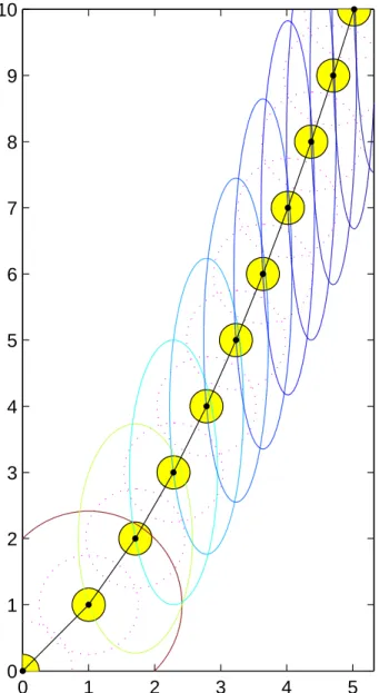
finite since 1 + 2η > 1. Figure 2.1 illustrates the sequence of quadratic models and the path of iterates for increasing k.
Cartis, Gould, Toint: Slow convergence of Newton’s method (draft) 4
0
1
2
3
4
5
0
1
2
3
4
5
6
7
8
9
10
Figure 2.1: Contour line of qk(x, y) = fk (full lines), the disks around the iterates of radius 14 (shaded) and 3
4 (dotted), and the path of iterates for k = 0, . . . 10.
2.3
Building the objective function
The next step in our example construction is thus to build a smooth function with bounded second and third derivatives (which implies that its gradient and Hessian are Lipschitz continuous) interpolating (2.3) at (2.6). The idea is to exploit the large components of the step along the second dimension (see (2.5)) to define f (x, y) to be identical to qk(x, y) in a domain around (xk, yk). More specifically, define,
for k ≥ 1, δ(α)def= 1 if 0 ≤ α ≤ 14, 16α3£−5 + 15α − 12α2¤ if 1 4 ≤ α ≤ 3 4, 0 if α ≥ 3 4. (2.9)
Cartis, Gould, Toint: Slow convergence of Newton’s method (draft) 5
This piecewise polynomial is defined(1) to be identically equal to 1 near the origin, and to smoothly
decrease to zero (with bounded first, second and third derivatives) between 1 4 and
3
4. Using this function, we may then define, for each k ≥ 0, a local support function
sk(x, y) def = δ µ° ° ° ° x − xk y − yk ° ° ° ° ¶ .
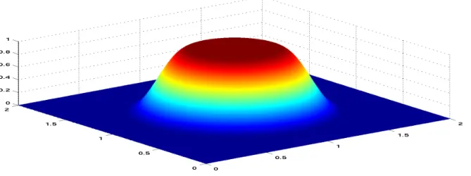
which is identically equal to 1 in a (spherical) neighbourhood of (xk, yk) and decreases smoothly (with
bounded first, second and third derivatives) to zero for all points whose distance to (xk, yk) exceeds 34. The shapes of a support function at (1, 1) is shown in Figure 2.2.
Figure 2.2: The shape of the support function centered at (1, 1) We are now in position to define the ’useful part’ of objective function as
fSN1(x, y) = ∞
X
k=0
sk(x, y)qk(x, y) (2.10)
for all (x, y) in IR2. Note that the infinite sum in (2.10) is obviously convergent everywhere as it involves at most two nonzero terms for each (x, y), because the distance between successive iterates exceeds 1. This function would already serve our purpose, as it obviously interpolates (2.3)-(2.4), is bounded below and has bounded first, second and third derivatives since the large values of qk(x, y) that occur in their
expressions always occur far from (xk, yk) and are thus annihilated by the support function.
However, for the sake of illustration, we modify fSN1(x, y) to build
fSN(x, y) = fSN1(x, y) + " 1 − ∞ X k=0 sk(x, y) # fBCK(x, y), (2.11)
where the background function fBCK(x, y) only depends on y (i.e., ∇xfBCK(x, y) = 0 for all x) and
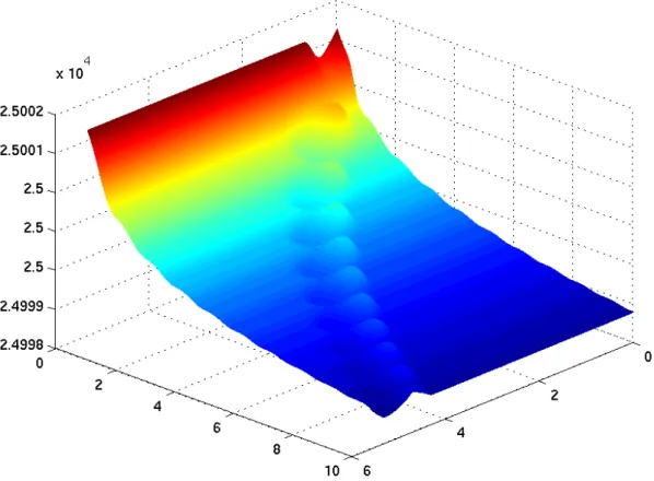
ensures that fBCK(x, yk) = fk for all x such that |x − xk| ≥ 34. Its value is computed, for y ≥ 0, by successive Hermite interpolation of the conditions (2.4) and
∇yfBCK(x, y) =
µ 1 k + 1
¶12+η
, ∇yyfBCK(x, y) = 0,
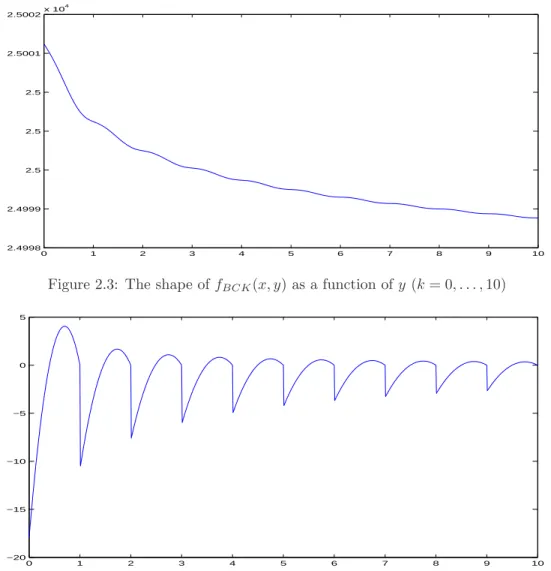
at yk = 0, 1, . . .. The shape of the resulting function as a function of y and of its third derivative are
shown in Figures 2.3 and 2.4, respectively. It may clearly be extended to the complete real axis without altering its smoothness properties.
(1)Using Hermite interpolation, with boundary conditions
δ(1 4) = 1, δ ′(1 4) = 0, δ ′′(1 4) = 0, δ( 3 4) = 0, δ ′(3 4) = 0, δ ′′(3 4) = 0.
Cartis, Gould, Toint: Slow convergence of Newton’s method (draft) 6 0 1 2 3 4 5 6 7 8 9 10 2.4998 2.4999 2.5 2.5 2.5 2.5001 2.5002x 10 4
Figure 2.3: The shape of fBCK(x, y) as a function of y (k = 0, . . . , 10)
0 1 2 3 4 5 6 7 8 9 10 −20 −15 −10 −5 0 5
Figure 2.4: The shape of the third derivative of fBCK(x, y) as a function of y (k = 0, . . . , 10)
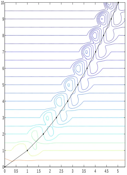
The modification (2.11) has the effect of ’filling the lansdscape’ around the path of iterates, consider-ably diminishing the variations of the function in the domain of interest. The countour lines of fSN(x, y)
as given by (2.11) are shown in Figure 2.5 on the following page, together with the iteration path. A perspective view is provided in Figure 2.6 on page 8.
3
Conclusions and perspectives
We have produced a two dimensional example where the standard Newton’s method is well-defined and converge slowly, in the sense that an ǫ-approximate first-order critical point is not found in less than ǫ−2iterations, an evaluation complexity identical to that of the steepest-descent method. The objective
function in this example has globally Lipschitz-continuous second derivatives, showing that this slowly convergent behaviour may still be observed under stronger but simpler assumptions than those used in Cartis et al. (2010). It is interesting to note that this example also applies if a trust-region globalization is used in conjunction with Newton’s method, since, because of (2.8), all iterates are very successful and the iteration sequence is thus identical to that analyzed here whenever the initial trust-region radius ∆0
is chosen larger than ks0k =
√ 2.
We also observe that the construction used above can be extended to produce examples with smooth functions interpolating general iteration conditions (such as (2.3)-(2.4)) provided the successive iterates remain uniformly bounded away from each other. Producing such a sequence of iterates from an original
Cartis, Gould, Toint: Slow convergence of Newton’s method (draft) 7 0 0.5 1 1.5 2 2.5 3 3.5 4 4.5 5 0 1 2 3 4 5 6 7 8 9 10
Figure 2.5: Contour lines of fSN(x, y) and the path of iterates for k = 0, . . . 10.
slowly-converging one-dimensional sequence whose iterates asymptotically coalesce can be achieved, as is the case here, by extending the dimensionality of the example.
Acknowledgements
The third author is indebted to S. Bellavia; B. Morini and the University of Florence (Italy) for their kind support under the Azione 2 “Permanenza presso le unita’ administrativa di studiosi stranieri di chiara fama” during a visit where this note was finalized.
References
C. Cartis, N. I. M. Gould, and Ph. L. Toint. On the complexity of steepest descent, Newton’s and regularized Newton’s methods for nonconvex unconstrained optimization. SIAM Journal on Optimization, 20(6), 2833– 2852, 2010.
Yu. Nesterov. Introductory Lectures on Convex Optimization. Applied Optimization. Kluwer Academic Publish-ers, Dordrecht, The Netherlands, 2004.
Cartis, Gould, Toint: Slow convergence of Newton’s method (draft) 8