Combination of Wireless sensor network and artifical neuronal network : a new approach of modeling

HAL Id: tel-01415333

https://tel.archives-ouvertes.fr/tel-01415333

HAL is a multi-disciplinary open access archive for the deposit and dissemination of sci-entific research documents, whether they are pub-lished or not. The documents may come from teaching and research institutions in France or abroad, or from public or private research centers.

L’archive ouverte pluridisciplinaire HAL, est destinée au dépôt et à la diffusion de documents scientifiques de niveau recherche, publiés ou non, émanant des établissements d’enseignement et de recherche français ou étrangers, des laboratoires publics ou privés.

Combination of Wireless sensor network and artifical

neuronal network : a new approach of modeling

Yi Zhao

To cite this version:

Yi Zhao. Combination of Wireless sensor network and artifical neuronal network : a new ap-proach of modeling. General Mathematics [math.GM]. Université de Toulon, 2013. English. �NNT : 2013TOUL0013�. �tel-01415333�

Combination of Wireless sensor

network and artificial neural network :

A new approach of Modeling

TH`

ESE

pr´esent´ee et soutenue publiquement le 12 D´ecembre 2013

pour l’obtention du

Doctorat de l’Universit´

e de Toulon

(sp´ecialit´e ´electronique, g´enie informatique, et traitement du signal)

par

Yi Zhao

Composition du jury

Pr´esident : M. le Professeur M. Cotsaftis Ecole Centrale d’Electronique Rapporteurs : M. le Professeur M. A. Aziz Alaoui Universit´e du Havre

M. le Professeur Cyrille Bertelle Universit´e du Havre Examinateur : M. le Professeur E. Moreau Universit´e de Toulon

Directeurs : M. Jean Marc Ginoux (MCF, HDR) Universit´e de Toulon M. Valentin Gies(MCF) Universit´e de Toulon

Remerciements

Je tiens à exprimer mes sincères remerciements et témoigner de ma grande re-connaissance à mon directeur et co-directeur de thèse M. Jean Marc Ginoux et M. Valentin Gies qui m’ont accueilli et soutenu pendant ces trois ans, qui m’ont encadré et motivé dans ce travail de recherche.

Je souhaite exprimer également ma gratitude envers tous les membres du jury. Merci particulièrement à M. le Professeur Michel Cotsaftis, qui a accepté de pré-sider le jury de cette thèse. C’est un honneur que MM. les Professeurs M.A. Aziz Alaoui et Cyrille Bertelle aient été les rapporteurs de ma thèse. Je souhaite expri-mer également ma gratitude envers tous les autre membres du jury, à la fois pour leur intérêt vis-à-vis de mes travaux de recherche, ainsi que pour les remarques et les discussions stimulantes lors de la soutenance.

Je remercie également M. Patrice Bendahan, Xavier Nesi et Christophe Lephay et les autres personnages de l’equipe ESPHI pour les passionnants échanges.

Je voudrais remercier M. le Professeur Yves Lucas et M. Stéphane Mounier de m’avoir accueilli au sein de laboratoire PROTEE. Merci pour leur soutien pendant ces trois ans.

Je voudrais remercier MM. les Professeurs Pascal Vincent, Stéphane Holé et Dr. Olivier Couture qui m’ont accueilli et soutenu pendant mon Master à UPMC (Université Paris VI) et ESPCI Paris Tech.

Je remercie également la Région PACA et l’entreprise ESPHI d’avoir financé ce travail, et je voudrais aussi remercier sincèrement à tous ceux qui ont contribué de près ou de loin à cette thèse et leur exprimer ma gratitude pour l’intérêt et le soutien qu’ils m’ont généreusement accordé.

Je remercie profondément mes parents, pour leur dévouement incessant durant ces années.

Enfin, l’itinéraire scientifique qui m’a amené à ce manuscrit et il aurait été in-concevable sans l’engagement de la France, de son Université et de ses collectivités territoriales que je remercie tout particulièrement.

à Mes parents ; à Fenghuan Ma ;

Résumé

Face à la limitation de la modélisation paramétrique, nous avons proposé dans cette thèse une procédure standard pour combiner les données reçues a partir de Ré-seaux de capteurs sans fils (WSN) pour modéliser a l’aide de RéRé-seaux de Neurones Artificiels (ANN). Des expériences sur la modélisation thermique ont permis de dé-montrer que la combinaison de WSN et d’ANN est capable de produire des modèles thermiques précis. Une nouvelle méthode de formation "Multi-Pattern Cross Trai-ning" (MPCT) a également été introduite dans ce travail. Cette méthode permet de fusionner les informations provenant de différentes sources de données d’entraî-nements indépendants (patterns) en un seul modèle ANN. D’autres expériences ont montré que les modèles formés par la méthode MPCT fournissent une meilleure performance de généralisation et que les erreurs de prévision sont réduites. De plus, le modèle de réseau neuronal basé sur la méthode MPCT a montré des avantages importants dans le multi-variable Model Prédictive Control (MPC). Les simula-tions numériques indiquent que le MPC basé sur le MPCT a surpassé le MPC multi-modèles au niveau de l’efficacité du contrôle.

Mots-clés: Réseaux de Capteurs sans fil (WSN), Réseaux de neurones artificiels (ANN), Modélisation, Formation croisée de Multiple source (MPCT) méthode, Les économies d’énergie, les performances de généralisation, Control Prédictif.

Abstract

A Wireless Sensor Network (WSN) consisting of autonomous sensor nodes can provide a rich stream of sensor data representing physical measurements. A well built Artificial Neural Network (ANN) model needs sufficient training data sources. Facing the limitation of traditional parametric modeling, this paper pro-poses a standard procedure of combining ANN and WSN sensor data in modeling. Experiments on indoor thermal modeling demonstrated that WSN together with ANN can lead to accurate fine grained indoor thermal models. A new training method"Multi-Pattern Cross Training" (MPCT) is also introduced in this work. This training method makes it possible to merge knowledge from different indepen-dent training data sources (patterns) into a single ANN model. Further experiments demonstrated that models trained by MPCT method shew better generalization performance and lower prediction errors in tests using different data sets. Also the MPCT based Neural Network Model has shown advantages in multi-variable Neural Network based Model Predictive Control (NNMPC). Software simulation and application results indicate that MPCT implemented NNMPC outperformed Multiple models based NNMPC in online control efficiency.

Keywords: Wireless Sensors Networks(WSN), Artificial Neural Networks (ANN), Modeling, Multi-Pattern Cross Training(MPCT) method, Energy efficiency, Gen-eralization performance, Model Predictive Control.

Table des matières

General introduction 13

1 Wireless Sensor Networks(WSN) . . . 13

2 Artificial Neural Network(ANN) . . . 15

3 Combination of WSN and ANN in modeling . . . 15

4 Outline of this Thesis . . . 17

Part I

The dynamic thermal behavior of Buildings

19

1.2 Physical phenomenon involved in buildings . . . 22

Chapitre 2 Mathematical model of a room 2.1 Thermal modeling of building . . . 25

2.1.1 Effective Indoor Thermal Time Constant(EITTC) . . . . 26

2.1.2 Mathematical model of room E106 in UTLN . . . 26

2.1.3 Limitation of the established mathematical model . . . . 30

Table des matières

Part II

Artificial Neural Networks and Wireless Sensor

Net-work

Chapitre 3

Neural Network Basics

3.1 Neural network basics . . . 35

3.2 Model of McCulloch-Pitts . . . 36

3.3 Perceptron . . . 36

3.4 The Delta Rule . . . 38

3.5 Multilayered Neural Network and Back-propagation . . . 41

3.6 Learning mode . . . 42

3.6.1 Activation functions . . . 42

3.7 Initializing the network’s weights . . . 44

3.8 Momentum . . . 44

Chapitre 4 The Back-Propagation algorithm 4.1 Back-propagation (BP) algorithm . . . 45

4.2 Practical aspects of the Back-propagation algorithm and Mo-mentum . . . 50

4.2.1 Procedure of network learning with Back-propagation . . 52

Chapitre 5 Overview of the WSN technology 5.1 Wireless Sensor Networks (WSN) . . . 53

5.2 A short history . . . 53

5.3 Applications of sensor network . . . 55

5.3.1 Military applications . . . 56

5.3.2 Environmental applications . . . 56

5.3.3 Health applications . . . 56

5.3.5 Other commercialized applications . . . 57

5.4 WSN topologies . . . 57

5.5 The Low power wireless technologies : A comparison . . . 58

Chapitre 6 Specification and Protocol 6.1 IEEE 802.15.4 and ZigBee . . . 61

6.2 IEEE 802.15.4 specification . . . 62

6.2.1 Network addresses of IEEE 802.15.4 . . . 62

6.2.2 The physical layer of IEEE 802.15.4 . . . 62

6.2.3 The MAC layer of IEEE 802.15.4 . . . 64

6.2.4 The frame format of IEEE 802.15.4 . . . 64

6.2.5 Functionality of units in IEEE 802.15.4 . . . 65

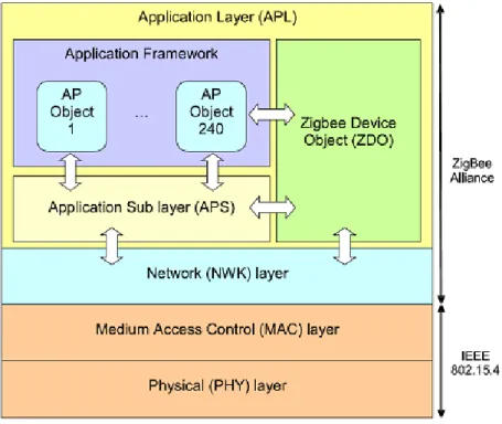
6.3 ZigBee . . . 65

6.3.1 Types of devices and the network topology of ZigBee . . 65

6.3.2 The stack ZigBee . . . 65

6.3.3 Configuration of a network ZigBee . . . 68

Chapitre 7 Development of a practical WSN system 7.1 WSN system development . . . 71

7.1.1 MRF24J40MA with PIC18LF4520 microcontroller . . . 72

7.1.2 Platform based on Freescale MC13224 . . . 75

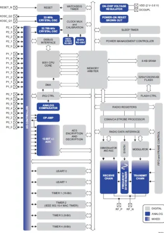
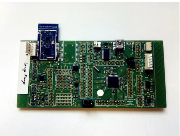
7.1.3 WSN solution with cc2530 microcontroller from TI . . . 79

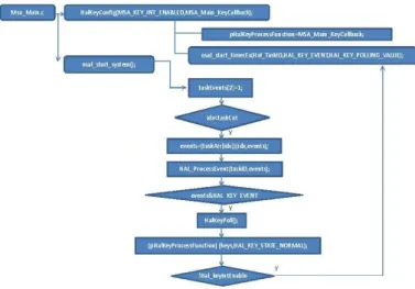
7.1.4 Z-stack of Texas Instrument . . . 85

7.1.5 The embedded system on CC2530 . . . 85

Chapitre 8 Feasibility of our WSN system : Link quality test 8.1 WSN in buildings : signal quality analysis . . . 91

8.1.1 Packet Error Rate (PER) test . . . 92

8.1.2 Signal strength indication and link quality indication . . 92

Table des matières

Chapitre 9

Hardware and Software solutions

9.1 Features of the developed Modeling software . . . 99

9.1.1 Graphical user interface Software design under C# . . . 100

9.1.2 The library "Aforge" and the implementation of ANN . 105 9.1.3 Advanced functions . . . 112

Part III

Combination of WSN and ANN :

A new approach of modeling

Chapitre 10

Combination of WSN and ANN

10.1 Combining WSN and ANN . . . 117

10.2 WSN based ANN thermal modeling . . . 117 10.2.1 Modeling experiments . . . 122 Chapitre 11

Multi-Pattern Cross Training

11.1 Principle and application of Multi-Pattern Cross-Training . . . 127

11.1.1 Optimum network training parameters with MPCT . . . 130 Chapitre 12

Model predictive control

12.1 Model Predictive Control (MPC) . . . 133 12.1.1 Principal theory of MPC . . . 133 Chapitre 13

Model predictive control using MPTC trained ANN models

13.1 ANN based model predictive control . . . 137 13.2 MPCT method based Model predictive control . . . 138

Part IV

Results and Perspectives

Chapitre 14

Results and Perspectives

14.1 Modeling results on prototype and buildings . . . 145

14.2 Energy efficient approaches . . . 152

14.3 Modeling results by applying MPCT method . . . 155

14.4 Model prediction control based on MPCT method . . . 158

Chapitre 15 Conclusion 15.1 Conclusion . . . 161

Annexe .1 Embedded code for MRF24J40MA and PIC18LF4520 . . . 164

.2 Main functions of Embedded code on MC13224 . . . 165

.3 Embedded code on CC2530 . . . 174

General introduction

Since the year of 1960, discussions have been made on the subject of non-parametric techniques against non-parametric techniques [1]. As a matter of fact, the discussions have motivated researcher and scientists from different domains inclu-ding finance, economics, pattern recognition, modeling, signal and image processing etc.

These preliminary discussions revealed their methodological differences : in para-metric techniques, a mathematical model (or statistical model) was developed for the problem from a statistical, geometrical, physical, or phenomenological perspec-tive. Although a relatively small number of unknown model parameters exist, they can be estimated from the data. These models are based on predefined rules as ma-thematical equations which can give a clear definition of the problem. It explicitly defines step-by-step tasks to achieve the desired results. This can be an ideal way to model a phenomenon when the rules relating to this problem is well known. In some practical cases, where the rules are either unknown or they are extremely difficult to be mathematically presented. Parametric modeling techniques do not meet these requirements and are not suitable as an appropriate solution [2, 3]. Artificial Neural Networks (ANN) is a typical nonparametric modeling technique. It is extremely useful in situations where the rules of the phenomena are either unknown or are too difficult to discover. Moreover, it is considered as an appro-priate solution for applications where the precision of traditional techniques cannot meet the requirements when a phenomena is too complex to be modeled with the well-defined rules [4].

1

Wireless Sensor Networks(WSN)

Wireless Sensor Networks (WSN) is considered as a significant technology ever since its birth, A wireless sensor network (WSN) consisting of autonomous sensor nodes can provide a rich stream of sensor data representing physical measurements. It can be described as a network of distributed self-powered nodes that could sense or exchange with environment. The main advantage of WSN is that it could be easily and rapidly installed and gather information for a long period of time, pro-viding an enormous quantity of sensor data. WSN based applications have shown a rapid growth in a variety of fields, including target tracking and surveillance, natural disaster relief, health monitoring, environment exploration and geological sensing, etc [5].

General introduction

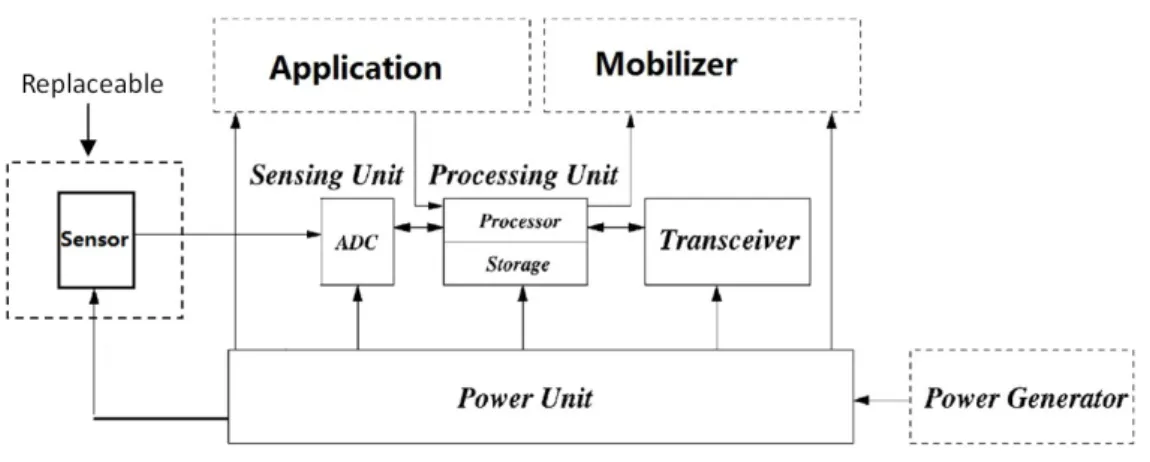
So far, most of the sensor networks deployed involve a relatively limited number of sensor nodes. They are usually connected to a central processing unit where all signal processing is performed [6]. On the contrary, the WSN is a wireless distribu-ted network, in which the signal processing is often done with acquisitions.

To better understand the necessity of deploying WSN in real applications, some description and statement should be made :

– Wireless

Cabled sensors networks work perfectly when nodes can be wired to stable energy sources and reliable infrastructure of communications. However, in many practical applications, the monitored target-area does not equipped any of these, for example, when the monitoring target is a group of wild ani-mals in the nature. Therefore sensor nodes should rely on local, finite, and relatively small energy sources as well as wireless communication channels, this would open a new door for wider applications with mobility and Auto-nomy.

– Distrubuted sensing

When a precise location of the interest-area is unknown in a surveillance zone, WSN allows a distribution of more autonomous sensors in the place closer to the wanted monitoring area. Instead of using only one or few sensors, this gives more signal to noise ratio (SNR) and better opportunities for the line of sight. SNR can be addressed in some cases by the deployment of a high sensitivity sensor, however, the line of sight of and more generally disturbance of noise cannot be processed by the deployment of a sensor with high sen-sitivity. Thus, distributed sensing provides more robustness under different environmental conditions.

– Distributed processing

It may be considered reasonable that in the cabled sensor networks, data can be communicated back to a central processing unit. However, for the sensor nodes of WSN, there are two main barriers : first, the finite energy budget is the first primary constraint. RF (Radio Frequency) Communication makes the main energy consumer. Secondly, most wireless sensor network defined limited data transmission rate. Thus, we need to process data as much as possible inside the network to reduce the energy consumption as well as the number of bits transmitted, particularly over longer distances.

2. Artificial Neural Network(ANN)

2

Artificial Neural Network(ANN)

Computer has become an necessary tool in engineering. Engineers have used various computer applications to improve their efficiency and performance. Ever since early 70s, Artificial Intelligence (AI) have been implemented by engineers to perform specialized tasks design.

Although computers are involved in a variety of engineering activities, currently, the main software applicable areas are with well-defined rules, such as the sophis-ticated analysis, graphic and CAD applications, etc. However, where there are no defined rules or heuristics, the use of computer is very limited.

Artificial Neural Networks (ANN) are another AI application that has recently been widely used to model nonlinear system, or system with unknown dynamics in many different domains of science and engineering [7]. ANN has been found to be extremely useful in situations where the rules are either unknown or are very difficult to explicit. Some of the main attributes of ANN can be listed as follows : – ANN can learn and generalize from examples to produce practical solutions

to problems.

– They can perfectly cope with situations where the input data of the network is unclear or incomplete.

– ANN are able to adapt solutions in time and to compensate from changing circumstances

– The data for training an ANN can be theoretical data, experimental data or empirical evidence based on reliable experiences.

ANN can be considered as a good generalized approximator based on the experience of a set of training data, it contains no explicit rules. Although it may not have the exact formality as the traditional parametric approaches, it is still A powerful tool that can produce perfect approximations when formal traditional solutions has difficulties with insufficient knowledge of the problem. It is chosen for applications where precision of traditional techniques can not meet the requirement that the problem is too complex to model with rules [4].

3

Combination of WSN and ANN in modeling

So far, WSN and ANN together have hardly been used in modeling. However, we think there are two main advantages of applying WSN and ANN in modeling and system identifications. First, the nature of WSN and ANN make them a combi-nation : WSN could be easily and rapidly implemented, providing a huge quantity

General introduction

of sensor data. These data sources can be essential for the ANN to identify a fine grained model. Second, they have high practical values : traditional mathematical modeling, Take the thermal modeling of building rooms as an example, approaches like [8] are usually established with well defined equations, they are usually used in general simulations instead of practical applications. It is mainly because these models are based on elements such as room thermal capacitances/resistance, air-flow rate, heat transfer coefficient, heat gain coefficient, etc. These parameters are difficult to measure precisely in buildings. Also, the dynamic behavior of some

phenomenon is very complex1_{, It is nearly impossible to obtain an accurate}

ma-thematical model with limited number of system parameters. The WSN system, on the contrary, is highly transplantable as it could be quickly equipped under any environmental surroundings to gather real-time thermal data. Additionally, with its self-adaptive learning and mapping ability, ANN can directly simulate the rela-tions between the modeling object’s inputs and outputs. Based on the two reasons, it seems that the combination of WSN and ANN can be a valuable and reasonable solution for modeling.

1. Here, the word "complex" refers to the complexity of the physical phenomenon, it differs from the definition of complexity in mathematics. The mathematical conception on complexity can be found in the following works [9, 10, 11].

4. Outline of this Thesis

4

Outline of this Thesis

This thesis is structured in four parts. In the first part of this thesis, we highligh-ted the limitations of traditional modeling methods by establishing and analyzing a mathematical thermal model of a building room. Instead ,we proposed to use WSN and ANN combined solution in building thermal modeling. The second part mainly introduces the concept and development of ANN as modeling tools and the WSN as our platform data acquisition. The wireless protocol and the design of embedded systems of our WSN system is systematically presented in this part. Also, we conducted experiments to show that our developed WSN system is re-liable for applications outside or inside the building. we introduced the software we developed for combining ANN and WSN in modeling, the main functions and features of this software has been highlighted.

In Part 3 of this thesis, we have shown the design of all our experiences in mode-ling the thermal response of a real building room with ANN and WSN. To improve the ANN thermal models’ generalization performance, we proposed a new training method called "Multi-Pattern Cross Training". It is able to merge knowledge from different training data patterns into a single ANN model. Thus, by exploring the general behavior of the phenomenon, it can be properly used to build a more com-plete model. We then presented the concept of Model Predictive Control (MPC) in which we focused on the neural network based MPC in the control of non- li-near processes. The necessity to use the MPCT method in MPC for optimizing the control efficiency is outlined in Part 3.

The results of WSN based ANN Modeling and the modeling performance with MPCT method are presented and discussed in Part 4, It is marked that MPCT method can be used to build models with better generalization performance, it also shows that MPCT method can improve the efficiency in Neural network based MPC. Some of our major embedded codes of the WSN system and is presented in the appendix of this thesis.

Première partie

The dynamic thermal behavior of

Buildings

1

The phenomenon involved in

building

1.1

Building Science : Thermal Phenomena

Buildings of residential and commercial facilities take about 40% of total energy consumption in Europe and USA. In China, residential urban energy consumption has tripled between 1996 and 2008 [12]. As a matter of fact, the energy consumption varies between different types of buildings. For example, buildings more than 30

years old consume from 300 to 400kW h/m2/year, while modern buildings consume

approximately from 150 to 200kW h/m2_{/year [13]. The improvement of energy}

efficiency in these old buildings can bring considerable environmental and financial benefits.

In order to find the best strategy to achieve energy efficiency, a basic understanding on the thermal behavior of buildings is necessary.

Chapitre 1. The phenomenon involved in building

1.2

Physical phenomenon involved in buildings

The three main physical phenomena involved in the thermal response of buil-dings are :

– Radiation : transferring heat from one object to another by electromagnetic waves (without contact).

– Conduction : the heat spreads within the material (solid, liquid, gas).

– Transport : The heat transfer between the air and the solid material resulting from the displacement of the particles (from the air) on the interface.

For a homogeneous material, we have the following equations to describe the be-havior of heat transfer through it. If the thickness of the material is T , the thermal resistance R considering the conductivity of the material λ is expressed by :

R = T

λ (1.1)

The heat transfer coefficient U2 _{is an indicator of energy efficiency. The value of U}

is expressed as the inverse of R :

U = 1

R =

λ

T (1.2)

For example, for a concrete wall (λ = 1.75W/mK) with a thickness of 0.3m, its thermal resistance has the value :

R = 0, 3

1, 75 = 0, 171m

2_{K/W (1.3)}

For a wall built of different materials, the overall thermal resistance is the sum of the resistances, and if we take into account the internal and external convection, we have here the overall thermal resistance :

R = n ∑ i=1 Ti λi + 1 hin + 1 hout (1.4)

The coefficients hin and hout are due to the internal and external convection

respectively.

Another important concept is the thermal inertia also known as thermal mass, it is a term used to describe the ability of materials to store heat (thermal storage capacity). The fundamental characteristic of any thermal mass materials is its abi-lity to absorb, store or release heat.

1.2. Physical phenomenon involved in buildings

Figure1.2 – Thermal resistance of a wall

Adding thermal mass in building’s insulated envelope can effectively reduce the extreme temperatures inside the building, making the most moderate average in-ternal temperature and comfort for habitants. Normally, building materials which can hold a heavy store of heat contain high thermal mass. On the contrary, the materials which is not capable of storing heat has lower thermal mass. In warm weather, the thermal mass at an initial temperature lower than the ambient air acts as a heat sink. By absorbing heat from the atmosphere, the temperature of the internal air reduce during the daytime. By releasing heat from the materials, the temperature of internal air drops slower. Thermal mass is particularly effective in areas where there is a large difference between the daytime maximum tempera-ture and minimum night temperatempera-ture.

The other important element is the solar radiation see Fig. 1.4, the heat inputs are generally two ways :

Figure1.3 – Temperature variations in the use of thermal mass

– Absorbed on the surfaces of wall, solar radiation is converted to heat stored in the walls.

Chapitre 1. The phenomenon involved in building

Figure1.4 – Solar radiation and indoor temperature

– The absorbed solar radiation through the transparent window is converted into heat in the ambient air.

2

Mathematical model of a room

2.1

Thermal modeling of building

Based on the description made in the previous chapter, the thermal response of building is related to many nonlinear and time varying effects such as the heat transport, convection, solar radiation, the interior charges, lighting equipment, cir-culation inside and outside air etc. The building room is a very complex thermal system, it is almost impossible to build a precise mathematical model with a limi-ted well characterized parameters.

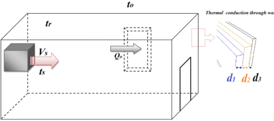
Fig. 2.1is presented as a mathematical model of the room E106 in the campus of Université de Toulon (UTLN), this room is equipped with a simple air conditioning as internal heating system and a vent pipe.

Chapitre 2. Mathematical model of a room

2.1.1

Effective Indoor Thermal Time Constant(EITTC)

The thermal time constant (TTC) can be used to quantify the thermal iner-tia of a building. In simpler words, it describes how the temperature varies under different thermal excitations. In previous works, the building TTC are calculated mostly with the thermal resistance and thermal capacitance of the building fabrics [14][15], Thus, these thermal constants are usually used to simulate the thermal response of buildings under environmental excitations. They can be very difficult to be used directly to characterize the indoor temperature changes in response to existing indoor heating/cooling system. Some of the thermal time constant are calculated based on major simplifications that all heat transport phenomena in building are linear [16] which can be limited facing the complex dynamic behavior of buildings. Thus, we proposed in this thesis a new concept : the Effective Indoor Thermal Time Constant (EITTC). By taking into consideration of both existing heating/cooling system’s performance and the building room’s thermal property. The EITTC can be used directly to characterize the indoor thermal response under existing indoor heating/cooling excitation and different outdoor conditions.

2.1.2

Mathematical model of room E106 in UTLN

In the mathematical model proposed by J. Florez and G.C. Barney [16], the thermal time constant Tr is described as :

dTr dt + Tr τr = Qh Cr + To CrRo + Tf CrRf (2.1)

where Tr is the room temperature, τr is the room thermal time constant. Qh is heat

source in the room, To is the out door temperature, Cr is the thermal flow store of

the room, R0 is the linear thermal dissipator from the room to exteriors, Tf is the

fabric (wall, roof) temperature, and the linear thermal dissipator from room to the fabric is Rf. The thermal time constant of the room can be written as :

τr =

CrRfRo Rf + Ro

(2.2)

where τr is the room thermal time constant, Cr is the thermal flow store of the

room, R0 is the linear thermal dissipator from the room to exteriors, and the linear

thermal dissipator from room to the building fabrics is Rf. This equation (Eq.(2.2))

is derived from a simplified linearized mathematical model of a room, it is much a general expression of room thermal constant. It can not be used directly to describe the indoor thermal response.

So, in order to characterize precisely the thermal response of the building room, in this thesis, a more detailed mathematical thermal model of building room is es-tablished :

2.1. Thermal modeling of building

According to the law of conservation of energy, the mathematical expression of this room model reads :

mncn dtn dt = ρsCsGs(ts− tn) + t0− tn R1 +t0 − tn R2 + t0− tn R3 + th− tn R4 + Qd (2.3)

where mncn is the heat capacity of indoor air (kJ/◦C), ts is the output air

tem-perature (◦C) from the air-conditioner, Gs is the volume of heated output air per

second(m3_{/s) ; t}

n, th, t0 are the indoor temperature, the adjoining room

tempera-ture and outdoor temperatempera-ture (◦C). ρs is the density of heated output air(kg/m3) ; Cs is the specific heat capacity of heated output air (KJ/(kg◦C)) ; R1, R2,R3,R4

are the thermal resistance of walls, windows, roof and the partition wall to the next door(k/kW ). Respectively, t0−tn R1 , t0−tn R2 , t0−tn R3 and th−tn

R4 are the thermal conduction

(kW ) on every part of the room. Qd is the sum of heat (kW ) emitted by the indoor

equipments and human bodies.

The incremental equation derived from Eq. (2.3) can be expressed as follows :

τd∆tn

dt + ∆tn= K1∆Gs+ K2∆Q (2.4)

where τ is the EITTC (s), K1 is the amplification factor of the indoor temperature

caused by heated air (◦C/(m3_{/s)) ; K}

2 is the amplification factor of indoor thermal

perturbation (◦C/kW ) ; ∆Q is the total change of the indoor heat (kW ). If the

temperature of heated air is defined as ts, we have : K2 = 1 ρsCsGs+ _R1₁ + _R1₂ + _R1₃ + _R1₄ , (2.5) τ = mncn ρsCsGs+ _R1₁ + _R1₂ + _R1₃ + _R1₄ = K2mncn, (2.6) K1 = ρsCs(ts− tn) ρsCsGs+ _R1₁ + _R1₂ + _R1₃ + _R1₄ = K2ρsCs(ts− tn), (2.7) ∆Q = ∆Qd+ ∆t0 R1 + ∆t0 R2 +∆t0 R3 +∆th R4 (2.8)

After performing a Laplace transformation of equation (2.4), we have the follo-wing equation :

Chapitre 2. Mathematical model of a room

If we define the delay between the thermal influences and indoor temperature variations as TR, the transfer function is obtained between the amount of heated

air and the changes of indoor temperatures read :

∆tn(S) ∆Gs(S) = K1e −Trs T1S + 1 (2.10)

In the same way, the transfer function between the thermal interference and indoor temperature reads.

∆tn(S) ∆qf(S) = K2e −Trs T1S + 1 (2.11)

If we consider that the volume of heated air GS is constant, we can find the

differential equations on the thermal response of the building room :

τ′dtn

dt + tn = K ′

1ts+ K2′qf (2.12)

In this equation, T₁′,K₁′,K₂′ are the same parameters as in Eq. (2.4).

τ′ = Mc ρscsGs+_R1₁ +_R1₂ +_R1₃ +_R1₄ = K₂′Mc, (2.13) K₁′ = ρscsGs ρscsGs+ _R1₁ + _R1₂ + _R1₃ + _R1₄ = K₂′ρscsGs, (2.14) K₂′ = 1 ρscsGs+ _R1 1 + 1 R2 + 1 R3 + 1 R4 , (2.15) qf = qn+ t0 R1 + t0 R2 + t0 R3 + t ′ n R4 (2.16)

And if we add the delay T_r′, we have the transfer function between the tempe-rature of the heated air and the tempetempe-rature of the room :

tn(S) ts(S) = K ′ 1e−T ′ rs T₁′S + 1 (2.17)

2.1. Thermal modeling of building

and the transfer function between the thermal interference and indoor tempe-rature : tn(S) qf(S) = K ′ 2e−T ′ rs T₁′S + 1 (2.18)

If the volume of heated air is considered as constant, we have

Gs= Gs0 (2.19)

where Gs0 is the volume of heated air at the start time.

If we compare from Eq. (2.4) to Eq. (2.12), we have :

T1 = T1′; Tr = Tr′; K1 = ts0− tn0 Gs0 K₁′; K2 = k′2 = 1 ρscsGs0 K₁′ (2.20)

Chapitre 2. Mathematical model of a room

2.1.3

Limitation of the established mathematical model

Two common problems with this type of models are : 1. the model is based on simplifications and it does not have the ability to provide accurate predictions in real time and it is hard to precisely measure all the parameters used in this model. 2. these models is only applicable for the specific modeled room, when the room changes, all the parameters and equations should be redefined. Thus, they are not practical.

For the first problem, as we explained in the introduction : for this type of mathematical modeling, the basic problem is that the number of parameters in-creases with the increase of problem’s complexity [3]. If we want to build a precise mathematical thermal model of the room, we have to take all the physical pheno-menon involved into the models, which means all the heat transferring, conduction, radiation. Furthermore, The thermal response of the room is related to the outside temperature, solar radiation, the interior equipment, lighting, human activity and the opening and closing of the door, etc. It is almost impossible to establish a precise mathematical model with a limited number of parameters. The complexity of this dynamic thermal response in the room will finally lead to a explosion of parameters in the correspondent mathematical model. This is the main reason that most of the mathematical room thermal models used in simulations are based on simplifi-cations [16] below regardless of the fact that these simplification has weakened the accuracy of models :

– All the phenomena of heat transfer are considered linear.

– Consider the room is a unique capability and neglect the content inside the room.

– neglecting the air flow inside the room.

– Suppose that the internal temperature is homogeneous.

The accuracy of the model can not be guaranteed due to the parameters : for example, parameters such as t0, t′n and Qn are time varying elements which is very

difficult to be measured in real time. Furthermore, the most basic parameters like thermal resistance, thermal capacity thermal mass are also difficult to be measured precisely. In addition to the difficulty of measuring these parameters.

The second simple and practical problem is that these models are not reusable, if the room changed, all the parameters have to be measured again due to different building fabrics and geometries.

2.2. Proposed new modeling method

2.2

Proposed new modeling method

In this thesis, the modeling solution combining WSN data and ANN is propo-sed to overcome the limitations of the traditional mathematical models introduced. ANN has been applied to improve the performance of WSNs [17]. However, We find that there is almost no previous research combined WSN data and ANN in mode-ling.

The two main advantages of applying WSN and ANN in building room thermal modeling. First, the nature of WSN and ANN make them a perfect combination : on one hand, WSN could be easily and rapidly implemented, providing a huge quantity of sensor data. These data sources in return could be essential for the ANN to identify a fine grained thermal model. Second, they have high practical values : as it is discussed, mathematical thermal modeling approaches are usually used in general simulations. They are hard to be applied in some practical appli-cations. The WSN system, on the contrary, is highly transplantable as it could be quickly equipped in any buildings to gather real-time thermal data. Additionally, with its self-adaptive learning and mapping ability, ANN can directly simulate the relations between building thermal affecting factors (heating source, solar radiation, outdoor temperature) and indoor temperatures. Based on the two reasons above, we believe that the combination of WSN and ANN can be a valuable solution for indoor thermal modeling.

Admittedly, some existing thermal modeling techniques exist, however, previous studies outlined that ANN model outperformed Auto-Regressive(ARX) models in predicting the indoor temperature because the ANN models are more sensible to the nonlinearities of the thermal effects in buildings [18][19]. Further more, J.W. Moon has pointed out in his previous work [20] that ANN’s adaptability makes it a more advantageous method in thermal control compare to Fuzzy method. Different techniques have their own advantages and shortcomings, here, it is ne-cessary to point out that the WSN and ANN combined modeling solution has a great advantage over the other modeling techniques : it is highly transportable and applicable under.

WSN as a very cheap, low-power, easy-to-use, miniature electronic devices can be installed quickly in most buildings while ANN’s universal approximating ability makes it possible in generating adaptive thermal models under different environ-mental and indoor conditions. This means the same system can be easily deployed anywhere without modifications in the hardware or software. We think the prac-ticality and wide-applicability of the proposed solution make it distinctive from other techniques.

Deuxième partie

Artificial Neural Networks and

Wireless Sensor Network

3

Neural Network Basics

3.1

Neural network basics

To understand the methodology that we present in this thesis, a systematic understanding of the neural network is necessary. In this section, we will focus on the conceptions and the development of artificial neural networks (ANN).

Neural networks is a kind of computing architectures inspired by biological brain [21] [22]. This kind of architectures are commonly called "connectionist systems", they consist of interconnected and interacting components named nodes or neurons. Neural networks are not characterized by explicit representation of knowledge or well defined rules of the problem, no symbol or values that correspond directly to classes of interest. Knowledge is implicitly represented in the diagrams of in-teractions between network’s components. Individual neuron in ANN emulate the biological neuron, it takes input data and make simple processing of it, selecti-vely passing on the processed data to other neurons (Fig. 3.1) Before sending out

Figure 3.1 – Comparison between a biological neuron and an artificial neuron

model

the processed data, each neuron use its "activation" function to format the data. Every neuron has its own weight values associated in the network, and these values

Chapitre 3. Neural Network Basics

determine at what level the input data are related to output data. Originally, a raw neural network only has a determined structure, and the weight values are usually random. The training of the network is a procedure that the network gets the knowledge from the data of experiences. The iterative repeat of training allows the network to determine its best fitted weight values (i.e., in image processing, a neural network can be trained to classify different images. Weight values are defi-ned during the training phase in which the network is taught to identify a image by the typical input image’s characteristics.).

Once the neural network is trained, it can be used to process new data. Useful summaries of fundamental neural network principles can be found in the relative works of Rumelhart etal. [23], McClelland and Rumelhart [24], Rich and Knight [25], Winston [26], Luger et Stubblefield [22], Gallant[27] and Richards and Jia [28].

3.2

Model of McCulloch-Pitts

In the 1940’s, McCulloch-Pitts network presented the beginning of Neural com-puting [29]. These connectionist networks are called "decision machines", as exem-plified in Fig. 3.2. A set of inputs is multiplied by the weights, and the outputs are then determined by simple logical or mathematical operations. In this way the input values are related to output values. McCulloch-Pitts networks are binary ; only 0 or 1 is the acceptable input form, also it is the standard format of output. The mechanism of McCulloch-Pitts network is simple : if the sum of the products of the inputs associated with weights is greater than or equal to 0, the output

returns 1, otherwise, 0. A threshold3 _{should be exceeded or equalled in order to}

have an output of the system 1. The rules used in mapping the input values to the output values, is the activation function which means that this function is used to determine the rules for the output node. McCulloch-Pitts networks can be used in logical computations (see Fig. 3.2) and they contributed to inspire further research into connectionist models during the 1950’s.

3.3

Perceptron

In the late 1950’s, a connectionist system with limited learning ability is develo-ped [30]. Rosenblatt created a new framework of neurons known as the perceptron (see Fig. 3.3). Like the network of McCulloch-Pitts, perceptron consists of binary activation functions and its binary output is determined by summing the products of its inputs and the weight values. Unlike the network of McCulloch-Pitts, a va-riable threshold value is used : if the linear sum of the input/weight products is greater than a threshold value (θ), the output of the system is 1, otherwise 0.

3.3. Perceptron

Figure 3.2 – McCulloch-Pitts’ neuron model

Chapitre 3. Neural Network Basics

3.4

The Delta Rule

Perceptron is a landmark on the road of Neural Networks. It is the beginning of making connectionist networks which is capable of mapping complex relations between inputs and outputs. By the end of 1950’s, the connectionist community reached the conclusion that connectionist models need more flexible learning rules. Thus, mathematical derivation has been introduced to the activations of the

net-work. The Delta Rule4 _{was then invented in the early 1960’s [31]. Although one}

may find this training rule is similar to the perceptron learning rule above [24]. The difference is that instead of using a threshold as the activation function, the delta rule uses a linear activation function for the output neuron. Further more, the differences of activations (network output) in every training iteration can be used to drive the learning. This is revolutionary comparing to all the connectionist’s networks before. The delta rule makes it possible to create self-adaptive neural networks. The network itself can now begin to update its weights by reducing the difference between target and actual output activations.

The data’s propagation through the network is presented below. Firstly, it will be normalized by the input layer neurons and multiplied by the associated weight. Then, the data are summed and reach to the output neurons where they are sent through an activation function, Finally, after the activation function, they become the output of the network.

yj = f ( n

∑

i

wijai) (3.1)

where n is the total number of input layer neurons, wij represent the weight

updating from the input layer neuron i to the output layer neuron j, ai is the the

activations function of the neurons in layer i, yj is the network’s output and f is

the activation function of the output layer.

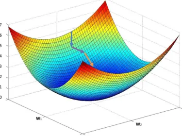
Given a training data pattern, the errors of the network is measured with the cost function (also called error function) (Fig. 3.4) [32]. The cost function is usually defined as the sum of the squares of the differences between all target outputs and actual network outputs (see Eq. (3.2)) The Delta Rule uses the gradient descent learning method to minimize the errors : the weights modified themselves along the direct path in weight-space, changes are applied to the weights proportionally to the negative direction of the derivation of the errors.

E = 1 2 p ∑ j=1 m ∑ n=1 (rjn− yjn)2 (3.2)

3.4. The Delta Rule

Figure 3.4 – The Delta rule in minimizing the error

where E is the total error, j is the number of all training patterns and n is the number of output neurons. A normalized form of E is given in the mean squared error (MSE) equation below :

M SE = Em = 1 2pm p ∑ j=1 m ∑ n=1 (rjn− yjn)2 (3.3)

where P is the total number of training data patterns and m is the total number of neurons in the output layer, the minimization of errors can be made in this way, for a given weight c :

δEm δwijc = δEm δyjz δyjz δwijc (3.4)

where yj sub z is the activation function for the node from the wij sub c, it can

be further expressed as :

δEm δyjz

Chapitre 3. Neural Network Basics and δyjz δwijn = δ δwijc m ∑ n=1 (wijnyin) = yic (3.6) we have then : δEm δwijx = (yjz − rjz)(yic) (3.7)

With the gradient descent learning method, the changes of weights must be proportional to the negative of Eq. (3.7), If a learning rate ϵ is introduced in Eq. (3.7), it can be re-written as :

∆wijx =−ϵ δE δwij

= ϵδaix (3.8)

Here, we take a simple example of using the Delta Rule to update weights of a neural network. The training data patterns which contain both inputs and outputs are presented in Table 3.1. The aim of training the network is to make it capable of labeling each of the four input cases in this table. This problem requires basically a network with four input nodes and one output node. If we define all the 4 weights associated with each input node are initially 0, and the learning rate ϵ is 0.25 During

Table 3.1 – Training data : Inputs and outputs samples

Training data Inputs Outputs +1 -1 +1 -1 1 +1 +1 +1 +1 1 +1 -1 -1 +1 -1 -1 -1 -1 +1 -1

the training, each training data pattern flows through the network individually, and weights update according to the Delta Rule : when the first training data pattern is given to the network, the sum equals 0. Because the target output for this training data set is 1, thus, the error is 1− 0 = 1. By applying Delta Rule, (see Eq. (3.8)), the changes of all the four weights in the network are calculated, the results is 0,25 ; -0,25 ; 0,25 ; -0,25. As the initial value of weights are 0 ; 0 ; 0 ; 0. Thus, the weights become 0,25 ; -0,25 ; 0,25 ; -0,25. When the second training data pattern is presented, the update of the weights are calculated as 0,25 ; 0,25 ; 0,25 ; 0,25. So the weights are 0,5 ; 0 ; 0,5 ; 0 after the second round of training, respectively, after

3.5. Multilayered Neural Network and Back-propagation

the third and the fourth pattern presented, the weight changes from 0.25 ; 0.25 ; 0.75 ; -0,25 to -0,375 ; 0,375 ; 0,875 ; -0,375, At the end of the irrelative training procedure, the total mean square error is :

Eq = (1)2+ (1)2+ (−1)2 + (−0, 5)2 = 3.25 (3.9)

At the end of this first iteration, it may be hard to realize that the error mini-mized alone with the changes of weights. However, with iterative flow of training, the error reduces. In this example, at the tenth iteration of training, the network successes in classifying all data patterns. At this moment, we can say that the net-work is well trained and it can be used to classify the data pattern with similar rules. For The Delta Rule, a basic requirement is the following : The rules consisted in the training data set should be linear [30]. This has greatly limited the use of Delta Rule, Minsky and Papert proposed multi-layer network to solve this pro-blem. However, they quickly realized that the use of linear activation function in Multi-layer neural networks is unable to solve the given problem. Functionally, a multi-layer neural network with linear activation functions is the same as a simple input-output network using linear activation functions. Two main questions are left for the connectionist community : "what kind of activation function should be used ?" and "how to train a multi-layer neural network ?" Blocked by these two questions, research of connectionist’s network has been freezed during the 70’s.

3.5

Multilayered Neural Network and Back-propagation

After almost ten years of depression in the connectionist’s community, a multi-layer neural network training algorithm has been proposed independently by Ru-melhart [23] and Yann Lecun [33]. The algorithm is known as the Back-propagation (BP). It uses error function of the Delta Rule and make these errors propagates backward through the network to update the weights matrix of the network. As BP is the most essential algorithm used in this thesis, a whole chapter is dedicated to it in order to give a detailed presentation of this algorithm.

Chapitre 3. Neural Network Basics

3.6

Learning mode

There are two main weights updating mode for neural networks : batch trai-ning, and on-line training. For batch traitrai-ning, the weight updates is carried out only when all the individual training data cases are presented to the network and the total error derivative is calculated [34]. On-line mode is also known as sequen-tial learning. It updates the weight value after each training data case submitted to the network.On-line learning is not a true gradient descent, because weights update slightly after each training data case presented to the network instead of updating with total derivative[34]. Normally, Batch learning need more memory capacity while on-line learning requires more weight updates. One advantage of online learning is that for online training, it is more likely to jump out of local minima during the training. Also, when high data redundancy exists training data patterns, the online training mode can be more efficient than batch mode [35]. In this thesis, we have chosen the online model for the network training because of these two advantages.

3.6.1

Activation functions

The most commonly used activations functions for connectionist’s network are presented below. They are respectively linear function, step function, sigmoid func-tion and bi-sigmoidal funcfunc-tion (see Fig. 3.5- 3.6). The mathematical expression of

Figure 3.5 – Activation function

these activation functions and their derivative are summarized below. The linear activation functions reads :

3.6. Learning mode

Figure 3.6 – Nonlinear activation function

The Binary Step Function with a threshold of θ reads :

f (x) =

{

1 if x≥ θ

0 if x < θ (3.11)

Binary sigmoid function and its derivative can be written as :

f (x) = 1

1 + exp(−σx) (3.12)

f′(x) = σf (x)[1− f(x)] (3.13)

While the bipolar sigmoid function and its derivation is expressed by :

g(x) = 2f (x)− 1 = 1− exp(−σx)

1 + exp(−σx) (3.14)

g′(x) = σ

2[1 + g(x)][1− g(x)] (3.15)

Bipolar sigmoid is also closely related to another activation function which is the hyperbolic tangent function :

h(x) = tanh(x) = exp(x)− exp(−x)

exp(x) + exp(−x) =

1− exp(−2x)

Chapitre 3. Neural Network Basics

A derivable non-linear activation function is required for a multi-layer neural network ; the purpose of this is to enable the use of gradient-descent method to trai-ning the network. The activation function most commonly used in BP networks is the sigmoid function which is the activation function used in this thesis.

3.7

Initializing the network’s weights

It is acknowledged that there is no determined rules to define initial values of weights in a neural network. In practice, it is normally random values that serve as the initial weight values. The random distribution can be used to avoid the local minima [27] during the network training. Usually, small values are recommended for the initial weights, Because high values can cause saturation of the activation function even at the beginning of the network [34]. Thus, in this thesis, we chose to use random small value for initial weights.

3.8

Momentum

Although by increasing the learning rate, the convergence speeds during the network training can be improved. Increasing learning rate can also lead to the in-stability of the network training based on gradient-descent. The weight values may oscillate erratically on the space of errors. For the back propagation algorithms, the employment of a momentum term is used to speed up the convergence and avoiding instability during the training. The momentum is defined as the product

of α5 by the previous weight update. With momentum, the network training can

be accelerated and it also avoided the oscillations of the weight[27]. Further intro-duction of momentum can be found in the next chapter where a Back-propagation Neural Network (BPNN) is used to show the effects of momentum during the net-work learning. In this thesis, we used the momentum term in our neural netnet-work model, the value of α by default is 0.9.

4

The Back-Propagation algorithm

4.1

Back-propagation (BP) algorithm

In this chapter, we will focus on the principle of back propagation algorithm (BP).

In 1974, Paul Werbos firstly presented in his work [36] how to make learning algorithm for a network (ANN can be considered as a special network). Unfortu-nately, the neural network community haven’t payed enough attention to his work at that epoch. In the mid 80’s, Back-propagation (BP) algorithm was invented by David Rumelhart[23] and Yann LeCun [33] independently. It rapidly gained a wide attention by the whole AI community and finally led the ANN research into a se-cond booming. BP algorithm can be considered as un improvement of Delta rules. It requires that each artificial neurons in the network uses the activation function which must be derivative. BP algorithm has been proved to be very powerful in training of Feed Forward Neural Networks (FFNN).

A FFNN using BP training algorithm is usually called as "Back Propagation Neu-ral Network (BPNN)." In the following, the term "BPNN" will be used for this type of neural network.

Here, we take a three-layered BPNN as an example, a typical network structure is presented here in Fig.4.1 below.

For a given neuron j in the output layer, we have its output error equals to :

ej(n) = dj(n)− yj(n) (4.1)

where dj(n) represents the target value of the network output from neuron j while yj(n) is the real network output on neurone j. So, we have the global error for the

whole output layer :

E(n)= 1 2 ∑ j∈C ej2(n) (4.2)

Chapitre 4. The Back-Propagation algorithm

Figure4.1 – Three layered Back-propagation Neural Network (BPNN)

is : Ej(n) = 1 N N ∑ n=1 E(n) (4.3)

the input of neuron j can be expressed as :

vj(n) =

∑

n

wji(n)yi(n) (4.4)

now, we have the output value from neuron j is :

yj(n) = σ(vj(n)) (4.5)

σ here is the activation function.

As the Delta Rules, BP algorithm tries to minimizer the error function E during the training of the network by updating the value in the weights matrix, the partial derivation of E by the weight wij is :

∂E(n) ∂wij(n) = ∂E(n) ∂ej(n) · ∂ej(n) ∂yj(n) · ∂ej(n) ∂yj(n)· ∂vj(n) ∂wji(n) (4.6)

In this equation above, we have :

∂E(n) ∂ej(n)

4.1. Back-propagation (BP) algorithm ∂ej(n) ∂yj(n) =−1 (4.8) ∂yi(n) ∂vj(n) = σ′(vj(n)) (4.9) ∂vj(n) ∂wji(n) = yi(n) (4.10)

Thus, we can rewrite the Eq. (4.6) uder the following form :

∂E(n) ∂wij(n)

=−ej(n)σ′(vj(n))yi(n) (4.11)

by consequence, the weights are updated by :

∆wji(n) =−η

∂E(n) ∂wij(n)

= ηej(n)σ′(vj(n))yi(n) (4.12)

where η is the learning rate and the local gradient is defined as :

δj(n) = ∂E(n) ∂vj(n) = ∂E(n) ∂ej(n) · ∂ej(n) ∂yj(n) · ∂yj(n) ∂vj(n) = ej(n)σ′(vj(n)). (4.13)

Thus, we have the final form of weights’ update (Eq. (4.12)) :

∆wji(n) = ηδj(n)yi(n) (4.14)

As neuron j belongs to the output layer of the network, the local gradient δj(n)

can be easily calculated according to Eq. (4.13). However, if neuron j belongs to one of the hidden layer, it can be difficult to obtain its local gradient, because there is no error value e(n) for the hidden layer neurons. A simple model is established in Fig. 4.2, the neuron j is now in the hidden layer while le neurone k is in the output layer. In this case, the local gradient can be put as :

δj(n) =− ∂E(n) ∂vj(n) = ∂E(n) ∂yj(n) · σ′_(v j(n)). (4.15)

Chapitre 4. The Back-Propagation algorithm

Figure 4.2 – Signal path when neuron j is in the hidden layer

The error function now becomes :

E(n)= 1 2 ∑ k∈C ek2(n) (4.16)

where C the collections of all output neurons in the network.

∂E(n) ∂yj(n) =∑ k ek(n) ∂ek(n) ∂yj(n) =∑ k ek(n) ∂ek(n) ∂vk(n) · ∂vk(n) ∂yj(n) (4.17) Here, ek(n) equals to : ek(n) = dk(n)− yk(n) = dk(n)− σ(vk(n)) (4.18) So, we have : ek(n) = dk(n)− yk(n) = dk(n)− σ(vk(n)) (4.19) ∂ek(n) ∂vk(n) =−σ′(vk(n)) (4.20)

4.1. Back-propagation (BP) algorithm vk(n) = m ∑ j=0 wkj(n)yj(n) (4.21)

Where m is the number of neuron in the hidden layer. So the derivation of vk(n)

by yj(n) is :

∂vk(n) ∂yj(n)

= wkj(n) (4.22)

Thus, Eq. (4.17) can be rewritten as :

∂E(n) ∂yj(n) =−∑ k ek(n)σ′(vk(n))wkj(n) =− ∑ k δk(n)wkj(n) (4.23) and we have : δk(n) = ek(n)σ′(vk(n)) (4.24)

Applying the above equations to Eq. (4.15), we have :

δj(n) = σ′(vj(n))

∑

k

δk(n)wkj(n) (4.25)

Now we have the local gradient of neuron j in the hidden layer. The mathema-tical procedure for calculating δj is represented by a graphical model in Fig. 4.3

below.

Now, as we already have the local gradient of neuron j in the hidden layer, we can calculate all the updated weight for all the neurons in the hidden layer by reapplying Eq. (4.14). the algorithm presented above is what we called Back Propagation.

Chapitre 4. The Back-Propagation algorithm

Figure 4.3 – Calculation of the local gradient of a neuron in the hidden layer

4.2

Practical aspects of the Back-propagation

al-gorithm and Momentum

The back- propagation algorithm presented in this chapter only requires the weights’ updates proportional to the derivation of the error functions (The gradient algorithm). The learning rate simply defines how much the weight changes on each training epoch. Therefore, swing weight is often caused by big learning rate. In practice, the best way is to use a reasonable value of learning rate without causing oscillation. As we explained in Chapter 3, a slight modification of BP algorithm is made that the previous weight update should influence the current weight update by using the Momentum.

With the momentum, once the weight starts to move in a particular direction, they tend to keep going in this direction. If there is a local minima presents, with enough momentum, the weights update can drive through the minima and stay in the right direction. Also, it helps to improve the speed of convergence during the training. The mathematical expression of momentum is :

∆wji(n) = αwji(n− 1) + ηδj(n)yi(n) (4.26)

where α is a positive value from 0 to 1, et η is the learning rate. Thus, we can rewrite Eq. (4.26) as follows :

∆wji(n)− αwji(n− 1) = ηδj(n)yi(n) (4.27)

4.2. Practical aspects of the Back-propagation algorithm and Momentum Finally we have : ∆wji(n) = η n ∑ t=0 αn−tδj(t)yi(t) (4.29) ∆wji(n) =−η n ∑ t=0 αn−t ∂E(t) ∂wji(t) (4.30)

Chapitre 4. The Back-Propagation algorithm

So, The function of momentum can be well explained by Eq. (4.30) : – if _∂w∂E(t)

ij(t) has the same sign for all t, |∆wji| grows, and it leads to a faster

convergence. – if _∂w∂E(t)

ij(t) alternates its sign in every iteration of training, |∆wji| changes in

small scale, which can lead to better stability.

The detailed description given in this chapter is necessary and essential to the fur-ther application of ANN in modeling with WSN data. In Chapter 5, a new training method for building a more comprehensive ANN model is proposed which is based on the Back-propagation.

4.2.1

Procedure of network learning with Back-propagation

While applying the BP algorithm in Neural Network training, there are basi-cally four phases : first, a case of training data is submitted through the network in a forward direction and finally become the output of the network. Secondly, errors are calculated based on the difference between of network output value and the target value, the weight updates of the output layer neurons are made at this point. Thirdly, the weights update propagate backwards to the preceding layer neu-rons. In this way, layer by layer, all the weight changes are calculated for the whole network. Finally, these calculated weight updates are implemented throughout the network. The next training iteration begins, and the entire training procedure is repeated.

5

Overview of the WSN technology

5.1

Wireless Sensor Networks (WSN)

December 18,2011, the "New York Times" published an article in which they presented the development of data monitoring and improvements in sensor tech-nology. The conclusion of this article is that the Internet will gradually departing from the scope of the consumer market and transfering to the physical world, which inevitably leads to the new era of "Internet of things".

The Wireless Sensor Networks (WSN) has been marked as one of the most revo-lutionary technologies ever since it was born. With great long-term economic and scientific potential, ability to transform our lives and bring new challenges in the future. A WSN consisting of autonomous sensor nodes which can provide a rich stream of sensor data representing physical measurements. They are deployed in many applications which rely on sensors to get the necessary information. In this thesis, an overview of wireless sensor networks as well as a systematic introduction of our developed WSN platform is presented.

5.2

A short history

The development of Network and its communication protocols can be traced back to the mid-1970s, since then, network communications has radically changed our lives [37].

– Ethernet

The Ethernet was developed in the mid 1970s by Xerox, DEC, and Intel, and was standardized in 1979. the official Ethernet standard IEEE 802.3 is re-leased by "Institute of Electrical and Electronics Engineers" (IEEE) in 1983. Data frames using the standard IEEE 802.3 have a variable length between 64 and 1514-byte per packet.

– Client-Server Network

Chapitre 5. Overview of the WSN technology

computers. Software designed for this kind of distributed computing network is separated into two different functionalities : Client-Server or we can call "front end to back end".

– P2P network and computing

P2P refers to Peer to Peer, it is a kind of architecture that all the units in the network share the same functionality. It uses simply bus topology to transfer files and change data. The mechanism of P2P computing is that it splits the computing tasks into pieces and spreads through the network. The results are then gathered for further processing. P2P computing has enlightened many internet applications since the 90’s.

– 802.11 Wireless Local Area Network. As known as the WLAN, IEEE released its standard ( 802.11 specification) in 1997, The current version is 802.11b which support a transmission rate up to 11M bit/s, The WiFi that we use in our daily lives for the PC, laptop, smart-phones is just based on this standard. – Bluetooth

Bluetooth is standardized by the specification IEEE 802.15 ; it is defined as Wireless Personal Area Network (WPAN). It is a short range RF techno-logy which provide wireless communication for electronic devices in a nominal range of 10m to 100m. It allows new devices to be hooked up easily to the net-work. Bluetooth uses 2.4GHz band with a transmission rate up to 1M bit/s. With the investments made in the 1970’s Defense Advanced Research Projects Agency-USA (DARPA) began the Distributed sensor Network (DSN) program in 1980. Since birth of DSN, Universities like Carnegie Mellon and Lincoln Labs of the Massachusetts Institute of Technology (MIT) have accelerated the research in this field.

Sensor networks have been deployed for monitoring applications such as forest fires detection, air quality qualification, weather stations and structural monitoring. Later, IBM and Bell Labs began to implement sensor networks in heavy industrial applications such as the distribution of energy, waste water processing and factory automation. However, at that time, the sensors were bulky and yet very expensive. They were difficult to meet the requirement of large-scale usage. The high cost of materials had prevented the sensor networks in wider applications.

Although sensor network for industrial and high-volume consumer applications was not possible during that period, both academic and industry have long recognized the potential of these networks

– UCLA, Wireless Integrated Network Sensors (1993)