Using 3D morphable models for 3D photo-realistic personalized avatars and 2D face recognition

(1)

HAL Id: tel-01777994

https://tel.archives-ouvertes.fr/tel-01777994

Submitted on 25 Apr 2018

HAL is a multi-disciplinary open access archive for the deposit and dissemination of sci-entific research documents, whether they are pub-lished or not. The documents may come from teaching and research institutions in France or abroad, or from public or private research centers.

L’archive ouverte pluridisciplinaire HAL, est destinée au dépôt et à la diffusion de documents scientifiques de niveau recherche, publiés ou non, émanant des établissements d’enseignement et de recherche français ou étrangers, des laboratoires publics ou privés.

Using 3D morphable models for 3D photo-realistic

personalized avatars and 2D face recognition

Dianle Zhou

To cite this version:

Dianle Zhou. Using 3D morphable models for 3D photo-realistic personalized avatars and 2D face recognition. Signal and Image Processing. Institut National des Télécommunications, 2011. English. �NNT : 2011TELE0017�. �tel-01777994�

(2)

Thèse de doctorat de Télécom SudParis dans le cadre de l’école doctorale S&I en

co-accréditation avec l’ Universite d’Evry-Val d’Essonne

Spécialité : Informatique

Par

M. Dianle ZHOU

Thèse présentée pour l’obtention du diplôme de Docteur

de Télécom SudParis

Les modèles déformables 3D (3DMM) pour des avatars personnalisables

photo-réalistes et la reconnaissance de visages 2D

Soutenue le : 5 Juillet 2011 devant le jury composé de :

Prof. DAOUDI Mohamed Telecom Lille1 Rapporteur

Prof. GARCIA Christophe Institut National des Sciences Appliquées _{(INSA) de Lyon} Rapporteur Prof. LELANDAIS Sylvie Université d'Evry-Val d'Essonne Examinateur

Prof. CHARBIT Maurice TELECOM ParisTech Examinateur

Prof. BAILLY Gérard CNRS/Universite de Grenoble Examinateur

Dr. Dijana Petrovska-Delacrétaz TELECOM SudParis Encadrant de thèse

Prof. Bernadette Dorizzi TELECOM SudParis Directeur de thèse

(3)

Using 3D Morphable Models for 3D Photo-realistic Personalized Avatars and 2D Face Recognition

by Dianle ZHOU

A dissertation submitted in partial satisfaction of the requirements for the degree of

Doctor of Philosophy in Informatique in the GRADUATE DIVISION of the

Universit Evry Val d’Essonne, TELECOM & MANAGEMENT SUDPARIS AND L’UNIVERSIT´E D’´EVRY-VAL D’ESSONNE

(4)

1

Abstract

Using 3D Morphable Models for 3D Photo-realistic Personalized Avatars and 2D Face Recognition

by Dianle ZHOU

Doctor of Philosophy in Informatique

TELECOM & Management SudParis and l’Université d’ Évry-Val d’Essonne Dr. Dijana Petrovska-Delacrétaz and Prof. Bernadette Dorizzi

In the past decade, 3D statistical face model has received much attention by both the commercial and public sectors. It can be used for face modelling for photo-realistic personalized 3D avatars and for the application 2D face recognition technique in biometrics. This thesis describes how to achieve an automatic 3D face reconstruction system that could be helpful for building photo-realistic personalized 3D avatars and for 2D face recondition with pose variability.

The first systems we propose Combined Active Shape Model for 2D frontal facial landmark location and its application in 2D frontal face recognition in degraded condition. We extend the original Active Shape Model by using the SIFT descriptor as a new local texture model and split the facial landmarks in facial internal region and fa-cial contour landmarks. The experimental results show that proposed Combined Active Shape Model algorithm is more robust for eyes and mouth center localization in more challenging lighting conditions, and also where some pose and expressions variabilities are presented.

The Second proposal is 3D Active Shape Model (3D-ASM) algorithm which is presented to automatically locate facial landmarks from different views. By taking advantage of 3D scans of face as training data, we propose to exploit 3D statical shape models and projective geometry across different views. The experimental results show that our proposed algorithm based on automatically generated training landmarks gives better performances than Combined Active Shape Model when large pose variation is

(5)

2

presented .

The third contribution is to use biomatrix data (2D images and 3D scan ground truth ) for quantitatively evaluating the 3D face reconstruction. During the experiment, the proposed two automatic facial landmark location algorithms are used to initialize our automatic 3D face reconstruction on the IV2 Multimodal Biometric Database and the results are compared with manual landmarks.

Finally, we address the issue of automatic 2D face recognition across pose. We follow the strategy proposed by Blanz et al.(Blanz 2003), which based on 3D face reconstruction, but using the 3D Active Shape Model landmark detector to automatic initialize the system. The 3D Morphable Model was used as a tool for correcting the pose of 2D images prior to presenting them to a face recognition algorithm. Experiments on the PIE database showed that the approaches proposed for pose correction improved the performance of a state of the art 2D face recognition algorithm when non frontal images were used on a system trained with near frontal images only. Although the experiment results are not out performance of the state of the art algorithm, but we have demonstrated in this chapter that we have studied in detail a version of an automated 3D Morphable Model based face recognition algorithm and discussed the issues related to its success and failure.

(6)

i

(7)

ii

Acknowledgments

During the five year of my study in France, I have read a lot of thesis. Each time I read one, I dream when I can have my one and how will I write the acknowledgements. And I didn’t understand why for each thesis there are the same word ”To my parents.”. Now I have my thesis and I have passed one third of my life. I begin to understand. They are the persons who bring me to the world, they are the person give me the life to understand.

I want to express my sincere thanks to my thesis advisor, Dr. Dijana Petrovska. Thanks for the guidance, for giving the chance to make my dream true, for the questions and for making me understand. We argued, we discussed and we tried to understand each other. That is the two different cultures and two different life. I want to say “we make the thesis” instead of “I make the thesis”.

I thank my thesis director, Prof. Bernadette Dorizzi. Its been an honour and pleasure to work with her. Her continuous guidance, constant support, and invaluable advice was instrumental for the success of this work.

I would like to thank Prof. Daoudi Mohamed and Prof. GARCIA Christophe for accepting to be a reporter for this thesis. I also thank Prof. LELANDAIS Sylvie, Prof. CHARBIT Maurice, Prof. BAILLY Grard for honouring me by being a part of the jury.

I also thank Prof. Gerard Chollet for his interest in my work and the critical comments he gave which helped me improve this work.

I also thank Prof. Guangjun Zhang who is my professor in China, for his support all the time.

I thank my former colleague, Dr. Mohamed Anouar Mellakh, who was a Ph.D researcher in our group during the first year of my thesis. His comments and suggestions were quite helpful. I also thank my other former collegues, Dr. Emine Krichen, Mr. Aurelien Mayoue, for helping me during my initial days. I also thank Dr. Sanjay Kanade for his help related to kindly help for my bad English and the way to do research. I also thank my other colleagues, Nesma, Guillaume, Walid, Dr Zhenbo Li,Dr. Quoc-dinh, Dr. Patrick Horain, David Gomez, Yannick Allusse, Aurelien Mayoue and our secretary Patricia Fixot, for their help and support.

(8)

iii

(9)

iv

5.5.1 Experimental Results of Face Identification with 3D Shape and Texture Parameters on subset of PIE database . . . 97 5.6 Viewpoint Normalization Approach. . . 98 5.6.1 Texture Extracted from Images or Synthesized Texture from 3DMM 98 5.6.2 Experimental Result . . . 101 5.7 Conclusions . . . 105

6 Conclusions and Future Work 106

6.1 Achievements and Conclusion . . . 107 6.2 Future work . . . 108

Bibliography 110

(12)

vii

List of Figures

2.1 Landmark positions and the contours of a 58-points template for facial analysis. . . 11 2.2 Difference of the Grey-Level Profile and the SIFT descriptor. Left: The

Grey-Level Profile (GLP) is extracted from the neighbourhood pixels per-pendicular to the contour. Right: The SIFT descriptor is computed over a patch along the normal vector at the landmark (the original image is from the BioID database [34]).. . . 16 2.3 Comparison of the Grey-Level Profile and the SIFT descriptor cost

func-tion from Eq 2.3. Left: Gradient profile matching cost of the landmark highlighted in Figure 2.2 over a window of size 21x21. Notice the multiple minima resulting in poor alignment of shapes. Right: SIFT descriptor matching cost for the same landmark point. . . 17 2.4 Combined landmark detection model: 45 landmarks define the facial

in-ternal region model (represented with SIFT features) and 13 landmarks define the facial contour model (represented with GLP features). . . 18 2.5 Combined Active Shape Model marching algorithm flow chart. . . 19 2.6 Typical fitting result of non frontal faces achieved by original ASM (top

row), SIFT-ASM (middle row) and C-ASM (bottom row). (The original images are from the IMM database [63]). . . 19 2.7 Annotated face image from the IMM face database [63]. . . 21 2.8 Comparison of the proposed Combined-ASM with already published

re-sults for eyes detections on the BioID database. . . 23 2.9 Cumulative histograms on FRGCv2.0 database with maximum eyes and

mouth error, the Stasm in this experiential we used the default training data (STASM-original). . . 25 2.10 Flow chart of the system for our fully automatic face recognition based

on C-ASM and global features. Images and video from MBGCv1 portal challenge [46]. . . 28 2.11 Typical landmark location results from the MBGCv1 portal challenge [46].

Top: landmark location results on still images. Bottom: landmark loca-tion results on video frames (Not all the video frame we have the same detection of landmarks, in here we just show some typical examples). . 29 2.12 The geometric and illumination normalization, image from [48]. . . 30 2.13 Images from the ”Video MBGC challenge” videos of enrolment (first 3

(13)

viii

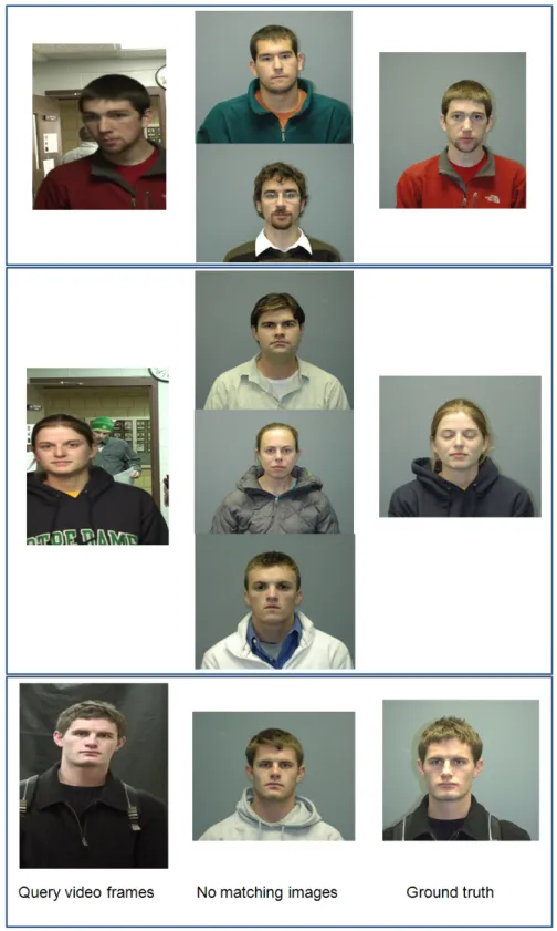
2.14 Example of biometric data extracted from the MBGCv1 - Portal Chal-lenge (http://www.nist.gov/itl/iad/ig/mbgc.cfm). . . 32 2.15 Some examples of wrong identified examples on MBGCv1 database. The

left column images are from the query video frame. The middle col-umn are the enrolment images of non-matching subjects to video, that produced a smaller similarity score than the corresponding enrolment im-ages of the subject. The right column are the corresponding enrolment images of the same subject. . . 34 2.16 Some challenging examples of enrolment still images from MBGCv2 database [46].

The images are too big (left) , to small (middle), or incomplete (right).. 35 3.1 Illustration of 3D Local Texture Model. For each landmark, one 2DLTM

is built separately for each viewpoint. 7 view-based 2DLTM compose our 3DLTM. . . 44 3.2 3D Morphable Model from [9] and the 58 manually selected 3D

land-marks. Middle: the average face model with 58 landland-marks. Left and right: Change the first component (±2δS1) of shape parameter and the

corresponding 3D landmarks. . . 49 3.3 Typical images from the IMM database [63]. . . 52 3.4 Images taken from all cameras of the CMU PIE database for subject

04006. The nine cameras in the horizontal sweep are each separated by about 22.5◦[60].. . . 53 3.5 Comparison of our 3D-ASM and Combined-ASM from Chapter 2 on the

BioID database for the two eyes. . . 54 3.6 Comparison of our 3D-ASM and Combined-ASM from Chapter 2 on the

subset of PIE Database. . . 55 3.7 Typical rotation images in PIE database [63]. From left to right image

are captured by camera: c37, c05, c29, c11. . . 55 3.8 The 3D-ASM facial landmarks detector point-to-point error distribution

on all 13 cameras on a subset of PIE database, for eyes and nose center points. . . 56 3.9 Comparison of 3D-ASM and Combined ASM on the subset of IMM

Database (80 images) on 58 landmarks. . . 57 3.10 Typically randomly generated 3D faces from 3D Morphable Model. . . . 59 3.11 Influence of the training data to 3D-ASM. Comparison of landmarks

loca-tion precision using different training data on the subset of IMM database. 60 3.12 Comparison of landmarks location precision using different view

cate-gories for training.Evaluated on IMM database. . . 60 3.13 Error analysis: Bad landmark location examples from IMM, BioID and

PIE database. . . 61 4.1 The framework of our automatic 3D face reconstruction algorithm from

a single image with nonfrontal face. By using the landmarks detected by 3D-ASM, the pose of the 3DMM and the main facial feature are recovered. Example input 2D image is from the PIE database [60]. . . 65

(14)

ix

4.2 The difference of the 3D landmarks and 2D landmarks. The left image is the rendering image with 58 landmarks on the 3D model. The right one is 2D image rendering in same angle, while with 58 2D landmarks manually located on 2D image. The red points show the significant different points. The 3D scan data are generated from USF database [57] . . . 71 4.3 Fitting a morphable model: analysis by synthesis iterations [10]. . . 74 4.4 The framework of our 3D face reconstruction evaluation protocol. The

in-put 2D image and the 3D ground truth scan are from the IV2 database [50]. 76 4.5 3D face reconstruction using three different landmarks for initialization.

First column: the input 2D image (above) and 3D ground truth scan (bellow). Second to fourth column: three different landmarks detected on the 2D image (above) and the corresponding 3D face reconstruction results (bellow), from left to right: CASM, 2D manual, 3D-ASM landarks. The input 2D image and the 3D scan are from the IV2 _{database [50].} _. ₇₉

4.6 Histogram of geometric Mean Squared Error distance from the 3D recos-ntructed models to the ground truth surfaces. . . 80 4.7 Typical examples of 3D face reconstruction from different view points.

The left column show the input images for face reconstruction. The sec-ond to the fourth columns present the correspsec-onding reconstructed 3D face rendered in frontal, side and profile view separately. . . 82 4.8 Examples of the synthetic head pose database for the evaluation of the

influence of the view point to the 3D face reconstruction precision. The top row are the synthetic image rendered by setting roll angle from 0 to 90 degree, 10 degree fro each image. The botton row are the synthetic image rendered by setting roll angle from 0 to −90 degree, 10 degree fro each image. . . 83 4.9 Evaluation result of the influence of the view point various to 3D face

reconstruction algorithm . . . 83 4.10 The influence of image quality to the 3D face reconstruction results. The

left column show the input images for face reconstruction with different quality. The second column is the reconstructed face rendering with the illuminate and pose parameters extracted from the input image. The third to the fifth columns list the correspondence reconstructed 3D face rendered in frontal, side and profile view separately. . . 84 4.11 Typical 3D face reconstruction results using 3D-ASM landmark lactation

for initialization. First column: the input 2D images. Second column: 3D reconstructed faces mapping with the texture from the 3DMM. Third column: 3D reconstructed faces mapping with texture extracted from the input 2D images . The input 2D images are from the IV2 database [50]. 86 5.1 Face reconstruction procedure. For each input image a shape α and a

texture β parameter vector can be extracted separately. . . 93 5.2 Images taken from all cameras of the CMU PIE database for subject

04006. The nine cameras in the horizontal sweep are each separated by about 22.5. . . 94 5.3 Flow charts of face identification across pose by viewpoint normalization

(15)

x

5.4 The different ways to map the texture, in the left column we give the original input image, those image are taken from the MBGCv1 database. In middle column we show the texture from the 3DMM with synthesis texture, in right column we show the mapping texture with the pixel from the input images. . . 99 5.5 Block diagram for pose normalization using 3DMM fitting and facial

sym-metry. Texture from the input image is extracted by projecting the ver-tices of the 3DMM on the image plan. If these verver-tices are visible, the RGB values will be taken and copied to the texture map which is pre-sented in cylindrical coordinates. The final texture is completed using symmetry property of faces. . . 100 5.6 Eyes and mouth based 2D pose correction Vs 3DMM-based Face Pose

correction. Images are taken from PIE database. . . 102 5.7 Face recognition performance comparison on PIE database. The first

row is the face identification rates using eyes and mouth based 2D nor-malization. While the second row is the face identification rates using 3DMM-based face pose correction. The third row we are using the same reconstruction step as the second row, the only difference is that texture for face reconstruction is synthesized from 3DMM instead of taken from input image. . . 103 5.8 Recognition accuracy comparison. In this figure, we compared our face

(16)

xi

List of Tables

2.1 Evaluation results on the BioID Database. Spatial error rate (at 10 % ) of eyes and mouth centers detection, of various landmark detection algorithms on the BioID database [34](in %). . . 24 2.2 Evaluation results on the FRGCv2.0 Database. Spatial error rate (at

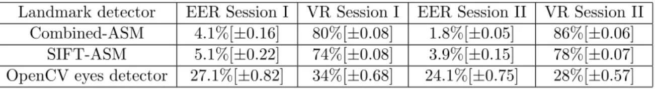
10 %) of eyes and mouth centers detection, of various landmark detection algorithms on the FRGCv2.0 Database [51]. . . 26 2.3 Face verification result on MBGCv1 portal challenge as a function of

EER. EER denotes Equal Error Rate and VR denotes face verification rate, SIFT-ASM denote the preliminary version of the proposed method (using only ASM with SIFT features.) The confidence interval at 99.9% [ ] is calculated as explained in [49]. . . 32 2.4 Error analysis on the MBGCv1 portal challenge using our automatic face

recognition system. . . 35 3.1 Evaluation results on the PIE Database. Mean error (in pixels) of eyes

and nose centers detection, of various different camera position. . . 56 4.1 Performance of the 3D face reconstruction initialized by 3D-ASM, CASM

and 2D manual landmarks in a side by side comparison. STD = standard deviation. . . 80 5.1 Face identification rate using ICP distance measure approach on PIE

database. . . 96 5.2 Face identification rate using parameters-based approach on PIE database. 97

(17)

xii

List of Abbreviations

ANR Agence Nationale de la Recherche EER Equal Error Rate

FAR False Acceptance Rate

FeaLingECc Feature Level Fusi on through Weighted E rror C orrection FRGC Face Recognition Grand Challenge

FRR False Rejection Rate

HTTPS Hypertext Transfer Protocol Secure

NIST National Institute of Standards and Technology SudFROG SudParis Face Recognition System

TLS Transport Layer Security ASM Active Shape Model AAM Active Appearance Model 3DMM 3D Morphable Model

PCA Principal Component Analysis LDA Linear Discriminant Analysis DLDA Direct Linear Discriminant Analysis LTM Local Texture Model

PDM Point Distribution Model C-ASM Combined Active Shape Model 3DASM 3D Active Shape Model

EBGM Elastic Bunch Graph Matching MES Mean Squared Error

(18)

1

Chapter 1

(19)

2

Human faces play an important role for face recognition, video games and animated movies. Faces are associated to people, who are related to key events and key activities happening from all over the world. There are many applications using face information as the key ingredient, for example, video mining, video indexing and retrieval, person recognition and so on. However, face appearance in real environments exhibits many variations such as pose changes, facial expressions, aging, illumination changes, low resolution and occlusions, making it difficult for current state-of-the-art face processing techniques to obtain satisfactory results in all these various conditions.

Using the face for recognition has a crucial advantage, since in principle it re-quires no cooperation of the subject to be identified. Also, face recognition research and technology have become increasingly important for better security scenario. Face recog-nition systems are useful for access control in controlled applications; however significant improvements in the technology are still required before it finds its way into everyday activities, such as identity checks on automated teller machines (ATMs) or recognis-ing offenders from public video surveillance. Furthermore, on the recently introduced biometric passports scheme by the International Civil Aviation Organization (ICAO)1, face recognition was selected as the global interoperable biometrics for machine-assisted identity confirmation after rating highest in terms of compatibility with key operational considerations of the scheme.

Another application of face processing is the field of face modelling for photo-realistic personalized representations. Modelling the behaviour of human face in some situations, or the effects on human face within some controlled environment is among the first useful areas that come to mind considering the necessity of computer generated and animated human face models. The film industry is also using related techniques with scenes that would be very dangerous or impossible to film with real actors.

As the face is so important for communication and the human brain is very talented to recognize, it’s realistic and detailed animation becomes a research area in computer graphics. We can see the results such as human body animations and talking heads. The animation of the face is mainly producing realistic facial expressions on the digital face model.

There are 2D and 3D face processing systems. In order to exploit the real

1

(20)

3

structure of the face, 3D data is more suitable, since the 3D nature of human face. Using 3D systems is more robust to the most critical factors limiting performance: illumination and pose variation compared to 2D system. Advantages for 3D based face processing systems are the following:

• The light collected from a face is a function of the geometry of the face, the albedo of the face, the properties of the light source and the properties of the camera. Given this complexity, it is difficult to develop models that take all these variations into account. Training using different illumination scenarios as well as illumination normalization of 2D images has been used, but with limited success. In 3D images, variations in illumination only affect the texture of the face, yet the captured facial shape remains intact.

• Another differentiating factor between 2D and 3D face processing is the effect of pose variation. In 2D images effort has been put into transforming an image into a canonical position. However, this relies on accurate landmark placement and does not tackle the issue of occlusion. Moreover, in 2D this task is nearly impossible because of the projective nature of 2D images. To circumvent this problem it is possible to use more different views of the face. This, however, requires a large number of 2D images from many different views to be collected. An alternative approach to address the pose variation problem in 2D images is either based on statistical models for view interpolation or on the use of generative models. Other strategies include sampling the plenoptic function of a face using light field techniques. Using 3D images, this view interpolation can be simply solved by re-rendering the 3D face data with a new pose.

But the 3D based system have their own problems compared to the 2D based systems:

• First is the acquisition, depending on the sensor technology used, where only parts of the face with high reflectance may introduce artefacts under certain lighting on the surface. The overall quality of 3D image data collected using a range camera is perhaps not as reliable as 2D image data, because 3D sensor technology is currently not as mature as 2D sensors’ technology.

(21)

4

• Another disadvantage of 3D face processing techniques is the cost of the hardware. 3D capturing equipment is getting cheaper and more widely available but its price is still significantly higher compared to a high resolution digital camera. Moreover, the current computational cost of processing 3D data is higher than for 2D data .

• Finally, one of the most important disadvantages of 3D face system is the fact that 3D capturing technology requires cooperation from a subject. As mentioned above, lens or laser based scanners require the subject to be at a certain distance from the sensor. Furthermore, laser scanners require few seconds of complete immobility, while a traditional camera can capture images from far away with no cooperation from the subjects.

In order to exploit this 3D structure in different applications, building a statistic 3D face model is a good choice. Once we obtain such 3D face models they can be used in different ways:

• 2D face recognition: A key example in the 2D face reconstruction using 3D statistical face model from single 2D image is the work from Blanz and Vet-ter(1999) [9]. But a lot of manual operations are needed. Such 3D models can be exploited in a generative way: thay can generate new synthesized 3D faces. We can used those 3D faces to train 2D landmark detectors which are robust to pose variation in order to avoid manual labelling of landmarks for better 2D face recognition. This is important for application where automatic facial landmarks detection and face recognition systems are needed. In chapter 5, we are trying to solve 2D face recognition problem with the priori of 3D knowledge of face. One challenging problem in 2D face recognition is the large pose variation on the face images. One way to solve this problem is the technique by Blanz et al. The human faces can be treated as a manifold surface in a 3D space. The 3D Mor-phable Model (3DMM) for face image synthesis and face recognition is developed by Blanz et al. [9,10]. One advantage of the 3D morphable face model is that it can easily handle variations on pose and illumination instead of 2D models. The variance of pose and illumination is always an obstacles for face recognition in 2D space. Another advantage of the 3D Morphable Model is that a 3D face surface is extracted from a single 2D face image, which avoids expensive 3D face/head

(22)

5

scan. Face recognition uses the shape and texture parameters of the model, which represent intrinsic information of faces. We can exploit 3D Morphable Model to reconstructed the 2D frontal image from the 2D nonfrontal image by using the priori of 3D knowledge of face.

• Photorealistic personalized representation: The 3D realistic avatar recon-struction (i.e. automatic 3D face reconrecon-struction from a 2D image) is a research area overlapping with computer vision, computer graphics, machine learning and Human-Computer Interaction (HCI). 3D face processing techniques are useful for (1) extracting information about the person’s identity, motions and states from images of face in arbitrary poses; and (2) visualizing information using synthetic faces for more natural human computer interaction. A general statement of the problem of 3D photorealistic personalized representation reconstruction can be formulated as follows: given still 2D image of a scene, the face is extracted from the image and reconstructed to be rotated and manipulated in 3D. The solution to the problem involves segmentation of faces (i.e. face detection) from clustered scene and localization of landmark points from face regions. This step contains the procedure of initialization of the 3D generic face model on the 2D image. In 3D face reconstruction step, the 3D statistic face model are modelled from mea-surements of faces, such as 3D range scanner data (i.e. 3D scans, 3D geometry and texture of neutral face) or images (i.e. 2D images or stereo images). Then, the 3D statistic face model is deformed according to the face in the 2D image to reconstruct a 3D face.

We are interested in this thesis in the reconstruction of 3D realistic face avatar from a 2D image. Given a single photograph of a face, we would like to estimate its 3D shape and texture by using 3D Morphable Model, its orientation in space and the illumination conditions of the scene. The face model created from the image can be then rotated and manipulated in 3D.

All the previous statements show the usefulness of 3D statistic model for face processing for a bunch of different applications. And it is also an actual problem and new proposal for quantitative evaluation on 3D face reconstruction are needed. In this thesis we evaluate the 3D face reconstruction in two different ways:

(23)

1.1. THESIS OUTLINE 6

• Quality evaluation: Taking the image and the 3D scan from the same subject, the 3D reconstruction precision could be evaluated by computing the geometric distance between the reconstructed 3D face and the ground truth (3D scan from the same subject).

• Indirect evaluation: The 3D face reconstructed algorithm also could be evaluated by 2D face recognition. As we discussed before, the 3D Morphable Model based 3D face reconstruction could be exploited to solve the 2D face recognition across pose problem. The better 3D face reconstruction precision we can achieved the better face recognition performance we can obtain.

1.1 Thesis Outline

This thesis is organised as follows: Chapter 2 presents the proposed Combined Active Shape Model for 2D frontal facial landmark location and its application in 2D frontal face recognition in degraded condition. In Chapter 3, we study the 2D facial landmark location on nonfrontal images, and details about the new construction, train-ing and fitttrain-ing of the proposed 3D Active Shape Model are given. It can be used for the initialization step for the automatic 3D face reconstruction. Since the training data of the 3D Active Shape Model are generated from the 3D Morphable Model, using it for initialization could benefit the 3D face reconstruction. In Chapter 4, our automatic 3D face reconstruction method is quantitatively evaluated with IV2 multimodel biometric database [50], by exploiting both 3D scans and 2D images. In Chapter 5, the method-ology of using the 3D Morphable Model to solve the 2D face recognition across pose problem is studied. The final chapter concludes the work of the thesis, and highlights directions for future work.

(24)

7

Chapter 2

Automatic 2D Facial Landmark

Location with a Combined Active

Shape Model and Its Application

for 2D Face Recognition

(25)

2.1. INTRODUCTION 8

2.1 Introduction

Finding the correct position of facial landmarks (key points) is a crucial step for many face processing algorithms such as face recognition, modelling or tracking. It is also needed for a variety of statistical approaches in which a model is built from a set of labelled examples. Also many 2D face recognition algorithms depend on a careful geometric normalization, with the location of landmarks such as eyes and mouth centres, that is previous to the global feature extraction step. With more reliable and more precise landmarks better face recognition performance is achieved.

Depending on the application context, face recognition can be divided into two scenarios: face verification and face identification. In face verification, an individual who desires to be recognised claims an identity, usually through a personal identification number, an user name, or a smart card. The system conducts a one-to-one comparison to determine whether the claim is true or not, i.e., face verification is to ask a question -“Does the face belong to a specific person?”. In face identification, the system conducts a one-to-many comparison to establish an individual’s identity without the subject to claim an identity, i.e., face identification is to answer the question - “Whose face is this?”. Throughout this thesis, the generic term face recognition is also used, which does not make a distinction between verification and identification.

The number and position of facial landmarks are not unique and depend on applications and algorithms. For 2D face recognition with global methods, usually eye centres, nose and mouth positions are needed. While for Active Shape Model (ASM) introduced by Cootes et al. in 1995 [19] approaches, the number of landmarks is bigger (around 50). They are located in regions of the nose tip, the nostrils, the center (iris) and corner of eyes, the mouth corners, the eyebrows and the tip of the chin. Those landmarks can be labelled by hand, but for realistic applications it is necessary to have automated methods. Due to the variety of human faces and their variability related to expressions, pose, accessories, or lighting and acquisition conditions, fully automatic landmark localization remains a challenging task.

This chapter focuses on automatic facial landmark location for face recognition, in situations where mainly illumination, scale and small pose variabilities are present. We are interested in automatic facial landmark location in 2D images for two purposes:

(26)

2.2. LITERATURE REVIEW ABOUT AUTOMATIC 2D LANDMARK

LOCATION 9

• To fully automate our 2D face recognition system.

• For 3D face reconstruction from 2D images.

The rest of this chapter is organized as follows: first, a brief literature review about facial landmark location is given in Section2.2. Then a reminder of the original Active Shape Model (ASM), on which our proposed combined model is based on, is given in Section2.3. The proposed Combined Active Shape Model, denoted as C-ASM, is explained in Section2.4. We evaluate the precision of the landmark detection in two ways. In Section2.5, we compare the detected landmarks with ground truth (manually annotated) landmarks. As we are interested in face recognition, in Section2.6, we use the C-ASM to do automatic landmark location for 2D face recognition. Finally, the conclusions related to this chapter can be found in Section2.7.

2.2 Literature Review about Automatic 2D Landmark

Lo-cation

A lot of algorithms have been proposed for facial landmark location for 2D images. As suggested by Hamouz et al.(Hamouz 2005) [30], they can be classified in two categories: image-based and structure-based methods.

In image-based methods, faces are treated as vectors in a large space and these vectors are furthermore transformed. The most popular transformations are Prin-cipal Components Analysis (PCA), Gabor Wavelets (Fasel 2002, Vukadinovic 2005) [24, 55,70], Independent Components Analysis (Antonini 2003) [3], Discrete Cosine Transfor-m (Salah 2006) [55], and Gaussian Derivative Filters (Arca 2006, Gourier 2004) [4,26]. Through these transforms, the variability of facial features is captured, and machine learning approaches like boosted cascade detectors (Viola 2001) [69], Support Vector Machines (Chunhua 2008) [21] and Multi-layer Perceptions are used to learn the ap-pearance of each landmark. Some examples of such methods are proposed by Viola and Jones [69], Jesorsky et al. [34], and Hamouz et al. [30].

Structure-based methods use prior knowledge about facial landmark posi-tions, and constrain the landmark searching by heuristic rules that involve angles, dis-tances, and areas. The face is represented by a complete model of appearance consisting

(27)

2.3. REMINDER ABOUT THE ORIGINAL ACTIVE SHAPE MODEL

(ASM) 10

of points and arcs connecting these points (Shakunaga 1998) [58]. For each point of this model, a feature vector is associated. Typical methods include Active Shape Models (ASM) (Cootes 1995, Ordas 2003) [19, 47], Active Appearance models (AAM) (Cootes 2004) [20], and Elastic Bunch Graph Matching (Wiskott 1997, Monzo 2008) [45, 73]. These methods are well suited for precise localization (Milborrow 2008) [44].

Within structure-based models, one outstanding approach is the Active Shape model (ASM) [20], because of its simplicity and robustness.

2.3 Reminder about the Original Active Shape Model

(AS-M)

The original Active Shape Model (ASM) was introduced by Cootes et al. in 1995 [19]. It is a model-based approach in which the priori information of the class of objects to is encoded into a template. Such template is user-defined and allows the application of ASM to work on any class of objects, as long as they can be represented with a fixed topology, such as faces.

The face template can be considered as a collection of contours, each contour being defined as the concatenation of certain key points defined in the shape analysis literature as landmarks, see Figure 2.1. The deformation of the landmarks allowed in the model template is learnt from a training database. As a result, an important property of ASM is that they are generative models. That is, once trained, ASM are able to reproduce samples observed in the training database and, additionally, they can generate new instances of an object not present in the database but consistent with the statistics learnt there from. In the original Active Shape Model (ASM) introduced by Cootes et al. in 1995 [19], there are two statistical models that exploit the global shape and the local texture prior knowledge in the segmentation process.That is Point Distribution Model (PDM) and Local Texture Model (LTM). The PDM represents the mean geometry of a shape and its statistical variations from the training set of shapes. While the LTM is used to describe the texture variations at each landmark position of the PDM.

(28)

(ASM) 11

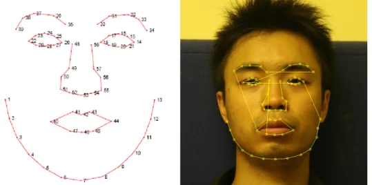
Figure 2.1: Landmark positions and the contours of a 58-points template for facial analysis.

2.3.1 Point Distribution Model

In order to construct the PDM, there is a need for a training set. The training set consists of a set of images, which represents the object class to be modelled. And those images should be annotated with the predefined template. The set of annotated landmarks on one image is referred to as the shape associated to that image.

The PDM is constructed by applying Principal Component Analysis (PCA) to the set of shapes in the training set. It is generally preceded by a 2D alignment in order to make the analysis independent from 2D rotation and scaling variations. Indeed, shape is usually defined as all the geometrical information remaining when positional, scaling and rotational effects have been filtered out from an object.

The Point Distribution Model is constructed by applying Principal Component Analysis (PCA) to the aligned set of shapes, which are presented by landmarks on the training face database. Assume there are N training images. The Point Distribution Model is a linear model, so the ith shape Si and the model parameters Pi in the shape space can be represented as follows:

Pi = ΦT(Si− S), Si = S + ΦPi, (2.1)

where i = 1, ..., N . S is the mean shape, and Φ is the eigenvector matrix of the shape space Briefly, the Point Distribution Model describes heuristic rules of the face shape. During the fitting, this model helps in the interpretation of noisy and low-contrasted

(29)

(ASM) 12

pixels.

2.3.2 Local Texture Model

As stated before, ASM have as many local texture models as the number of landmarks in the template. A typical image structure that describes the local tex-ture around each landmark is the Grey-Level Profile (GLP) [19], calculated from the fixed-length pixels sampled around each landmark. The direction of the profile is per-pendicular to the contour. The first derivative of the profile is calculated and used as the feature vector. Those vectors are extracted from all the training images, and represent the normalized derivatives profiles, denoted as g1, g2, ..., gN. The mean profile g and the covariance matrix Cg are computed for each landmark. The Mahalanobis distance measure is used to compute the difference between a new profile and the mean profile g, defined as follows:

M h2(gnew) = (gnew− g)Cg−1(gnew− g)T. (2.2)

Actually different Local Texture Models are adapted to different conditions, the examples are introduced in the following Subsection 2.3.3. The dimension of the GLP is depended on the number of fixed-length pixels sampled around each landmark, the details about the parameters will be explained in Section2.5.

2.3.3 Matching algorithm

As explained in Cootes et al. [20] and Sukno (Sukno 2007) [65], when the shape models are used for segmentation and landmark location, only two inputs are required: an image containing a face and a starting guess of the face position (i.e. provided by a face detector). The matching process alternates image driven landmark displacements and statistical shape constraints based on the PDM, usually performed in a multi-resolution fashion in order to extend the capture range of the algorithm. The matching process can be summarized in the following steps:

1. Place a first guess of the model into the image (generally, a scaled version of the mean shape, depending on the application task).

(30)

(ASM) 13

2. Search the image in the neighbourhood of each landmark. Adjust the coordinates of each landmark to the best position in this neighbourhood. In other words: move the landmarks according to their LTM. This will generate a cloud of points without shape constraints.

3. Apply shape constraints: find the best plausible shape matching the cloud of points generated in step 2. This implies finding the model parameters and some transformation (e.g. a similarity) from model coordinates to image coordinates. The Sconstrainparameter restricts the PCA coefficients to lie within Sconstrain(For example,Sconstrain= 3 ) times the standard deviation observed in the training set.

4. Go back to step 2 until stop condition is reached.

The criterion used to displace the landmarks at step 2 is the minimization of the Maha-lanobis distance based on the Gaussian model learnt during training for each LTM. Let {g_j(1), gj(2), ..., gj(kP)} be the set of local texture points for kp candidate positions at landmark j. The position suggested by the LTM will be the one minimizing:

M h2(gj(k)) = (gj(k) − gj)C_g−1(gj(k) − gj)T (2.3)

for k varying between 1 and kp, where M h2 denotes Mahalanobis distance Once all landmarks have been displaced to their best local position, they form a cloud of points which not necessarily describe a plausible shape for the studied object (i.e. a human face).

At step 3, shape restrictions are applied according to the PDM. As a result, landmarks are displaced again to the nearest plausible shape to the candidate points provided by the appearance models (in a least squares sense). The rationale behind shape restrictions is the assumption that facial shapes lie approximately within a hyper ellipsoid (in PCA-space) that can be learnt during training. However, for simplicity reasons it is very common to use PDM and limit the shape-space to a hyper-cuboid.

Starting from the original formulation of ASM introduced above, a considerable number of extensions have been proposed. One of the most interesting aspects of the original formulation of ASM is its simplicity. For example, the residuals of the shapes with respect to the mean are assumed Gaussian. This formulation works well for a wide variety of examples, although it is too simple to represent nonlinear shape variations.

(31)

2.4. A COMBINED ACTIVE SHAPE MODEL FOR LANDMARK

LOCATION 14

Non linear formulations of the PDM were proposed by Sozou et al. in 1995 [62] using Multi-Layer Perceptron (MLP) to perform the PCA decomposition. The experiments reported on image search revealed comparable performance to the linear PDM, yet requiring half the number of dimensions. Chen et al. in 2004 [18] focused on a different aspect of the PDM. They decomposed the overall error of ASM fitting into two terms: representation error and search error. They analysed the behaviour of the error as a function of the variance explained by the model. Based on experiments over 400 faces they claim that the optimal percentage of variance retained by the model is lower than that generally employed.

As opposed to those modifying the PDM, a number of authors have focused on the texture model of ASM. Wang et al. in 2002 [71] combined the first order derivatives with edge information to work with facial images and Koschan et al. in 2002 [37] explored inclusion of color information. While Ordas et al. in 2003 [47] replace the 1D normalized first derivative profiles of the original ASM with local texture descriptors calculated from “locally orderless images”, for reliable segmentation for cardiac Magnetic Resonance data. In Milborrow et al. in 2008 [44], the authors use the 2D profile in the square region around the landmark for a more precise fitting result.

However most of the research in this topic has concentrated in improving the precision of landmark detection in “passport” like images. As we also are interested in noncollaborative environments, we propose two extensions to increase the robustness under degraded conditions. First, we replace the gray-level profiles with SIFT features as LTM; second in order to have a better representation of faces, the landmarks on the face region and the face contour are modelled and processed separately for the PDM.

2.4 A Combined Active Shape Model for Landmark

Loca-tion

2.4.1 Using SIFT Feature Descriptor as Local Texture Model

Some previous work exist that try to choose better Local Texture Models. Different Local Texture Models are adapted to different conditions. For example, using the gray-level profiles is simple and fast and suitable for real-time processing, but it is less precise. While the 2D profile in the square region around the landmark used in

(32)

LOCATION 15

[44] is precise in controlled conditions. As we are more interested in non collaborative environments, such as video-based face recognition, we propose to use the SIFT [?,42, ?, ?] feature descriptor, which is robust to degraded conditions, such as illumination or small pose variations.

Scale Invariant Feature Transform (SIFT) Features

In 2004, David Lowe presented a method to extract distinctive invariant fea-tures from images [42]. He named them Scale Invariant Feature Transform (SIFT). The process consists of four major stages: (1) scale-space peak selection, (2) key point lo-calization, (3) orientation assignment, and (4) key point descriptor. In the first stage, potential interest points are identified by scanning the image over location and scale. This is implemented efficiently by constructing a Gaussian pyramid and searching for local peaks (termed key points) in a series of Difference-of-Gaussian (DoG) images. In the second stage, candidate key points are localized to sub-pixel accuracy and elimi-nated if found to be unstable. The third step identifies the dominant orientations for each key point based on its local image patch. Finally, local image descriptors are built for each key point. Local gradient data is used to create key point descriptors. The gradient information is rotated to line up with the orientation of the key point and then weighted by a Gaussian with variable scale. This data is then used to create a set of histograms over a window centred on the key point. Key point descriptors typically use 16 histograms, aligned in a 4x4 grid, each with 8 orientation bins, one for each of the main compass directions and one for each of the mid-points of these directions, resulting in a feature vector containing 128 elements. In our application we use this SIFT local image descriptor as our Local Texture model. In this thesis we implement the SIFT descriptor ourself.

Advantages of the SIFT Feature Descriptor

Using SIFT features for object matching is very popular, because of SIFT’s ability to find distinctive key points that are invariant to location, scale and rotation, and robust to affine transformations (changes in scale, rotation, shear, and position) and changes in illumination [42]. It seems to be a reliable choice for solving the problem of illumination and pose variability during the facial landmarks location. Since it is based

(33)

LOCATION 16

on the local gradient histograms around the landmark, the SIFT descriptor is highly distinctive and partially invariant to variations, like illumination or 3D view point, as introduced in [42]. In our application, we use the SIFT descriptor to replace the Grey-Level profiles. In order to make the ASM shape model rotation invariant, the gradient orientations of the descriptor are always computed relative to the edge normal vector at the landmark point which could be obtained by interpolation of neighbouring landmarks, as depicted in Figure2.2.

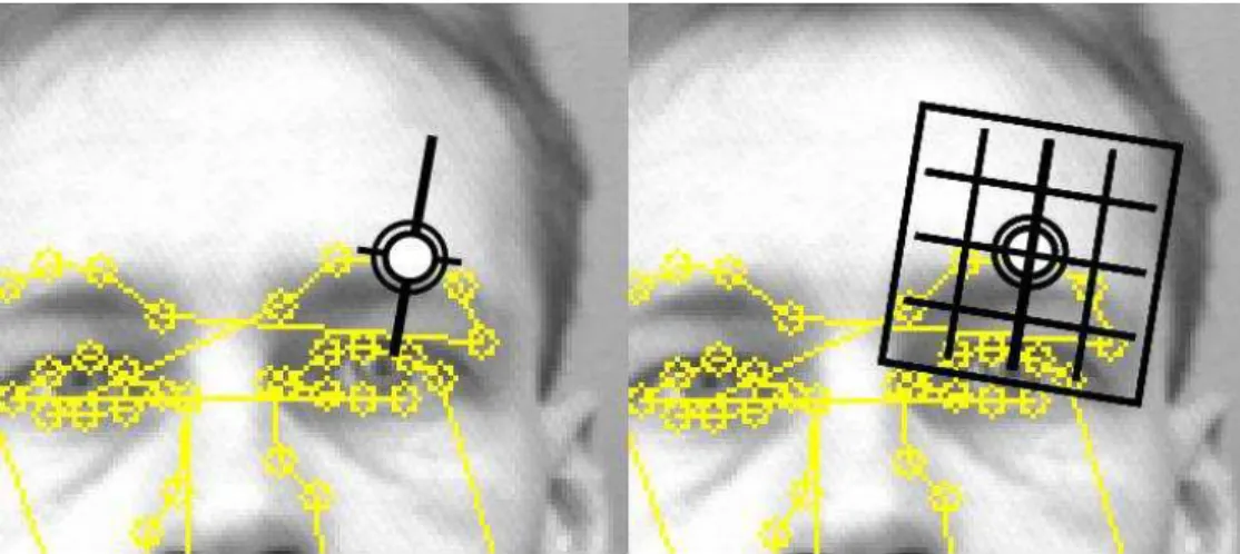
Figure 2.2: Difference of the Grey-Level Profile and the SIFT descriptor. Left: The Grey-Level Profile (GLP) is extracted from the neighbourhood pixels perpendicular to the contour. Right: The SIFT descriptor is computed over a patch along the normal vector at the landmark (the original image is from the BioID database [34]).

There are the two main advantages of the SIFT feature descriptor. The first advantage is that SIFT descriptors encode the internal gradient information of a patch around the landmark, thus capturing essential spatial position and edge orientation in-formation of the landmark while Grey-level Profile only captures the one-dimensional pixel information that is perpendicular to the contour. Though the Mahalanobis dis-tance measure assumes a normal multivariate unimodel distribution of Grey-level Pro-file, in practice, they can be any statistical distribution. The SIFT descriptors have a more discriminative likelihood model which is distinctive enough to differentiate between landmarks.

In Figure.2.3, we calculated the Mahalanobis distance of the neighbourhood points over a 21x21 pixels window around the landmark highlighted in Figure.2.2. The SIFT descriptor has a unambiguous minimal point in the center of the neighbourhood

(34)

LOCATION 17

Figure 2.3: Comparison of the Grey-Level Profile and the SIFT descriptor cost function from Eq2.3. Left: Gradient profile matching cost of the landmark highlighted in Figure 2.2over a window of size 21x21. Notice the multiple minima resulting in poor alignment of shapes. Right: SIFT descriptor matching cost for the same landmark point.

region, while the results of GLP contains more noises. Also the SIFT descriptors are invariant to affine changes in illumination and contrast by quantizing the gradient orien-tations into discrete values in small spatial cells and normalizing these distributions over local blocks. Such features are important in challenging real-life situations presenting illumination variabilities.

The second advantage of the SIFT descriptors is that they are more stable to changes that occur due to changes of pose, that can occur when dealing with faces .

2.4.2 Combined Active Shape Model (C-ASM) Based on Facial Inter-nal Region Model and Facial Contour Model

One of the novity of our work is applying different feature descriptor for differ-ent landmarks on the faces.As shown above, using SIFT feature descriptor, we can find correspondences between landmarks in two images that have small pose variability, even when the landmarks used to train the ASM are in 2D. The points in the face region that we denote as “internal” (such as eyes’ corners), could be considered as the perspective projection of 3D face on the image plan. While the contour points are different, and are more dependent on the 3D view point. In that case the SIFT descriptor dose not work when the acquisition angle of testing images is different from the training images. Especially when those points are occulted because of minor head pose rotation, see Figure2.6.

(35)

LOCATION 18

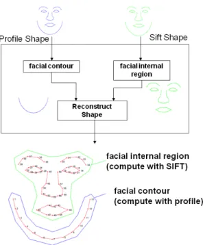
So in our proposed approach, two models are used to represent the human face. One model represents the landmarks of what we call “internal region”, including the landmarks on the eyes, nose, eyebrows and mouth. Those points could be considered as 3D position invariant during perspective projections. So we use the SIFT descriptor for this model, and we name it facial internal region model. The other one models the contour point on the face only. For those points using SIFT representations will result in wrong matches. The gradient of the profile is more suited for the contour points, so we use Grey-Level Profile to describe them, and we name it facial contour model.

Figure 2.4: Combined landmark detection model: 45 landmarks define the facial inter-nal region model (represented with SIFT features) and 13 landmarks define the facial contour model (represented with GLP features).

The facial internal region model is represented with 45 points, while 13 points are used for the facial contour model, as depicted in Figure.2.5. Each of them has its own shape model and shape variability. The combination of the two models makes the final results.

In the fitting step, for each iteration the two models are matched to the face image separately. After matching, we combine them into a new face model and use the Point Distribution Model to constrain it to a plausible shape in the shape space,

(36)

LOCATION 19

Figure 2.5: Combined Active Shape Model marching algorithm flow chart.

Figure 2.6: Typical fitting result of non frontal faces achieved by original ASM (top row), SIFT-ASM (middle row) and C-ASM (bottom row). (The original images are from the IMM database [63]).

(37)

2.5. EXPERIMENTS FOR C-ASM LANDMARK LOCATION

PRECISION EVALUATION 20

as shown in Figure.2.4. This is repeated iteration by iteration at each resolution until convergence is reached.

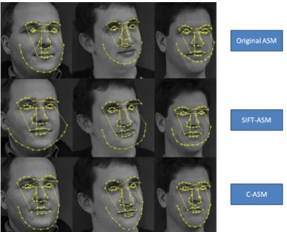
In Figure.2.6, for comparison purposes, we show on the first line the results of the automatic landmark detection with the original ASM (using only profile features), the ASM that is based on SIFT features (middle row), and the result of our Combined Active Shape Model (C-ASM). We can observe that the Grey-Level Profile has better performance on the contour points of side-view images, while SIFT features seem to be more adapted for the internal face region points. But we should note that, the idea to use the Gray-level Profile as the LTM for the facial contour is not only to improve the precision of the detected landmarks on the contour, but also to constrain the contour points around the mouth. This will increase the robustness of the landmarks on the facial internal region such as mouth and eye, as shown in Figure2.6, which are the points needed for face normalisation in the applications of face recognition. The experimental results for face recognition are given in Section2.6.

2.5 Experiments for C-ASM Landmark Location Precision

Evaluation

In this section, we compared the detected landmarks with ground-truth (man-ually annotated) landmarks. We are mostly interested in automatically detecting the two eyes and mouth centres which are used for our face normalization step for our face recognition system explained in Mayoue et al. in 2009 [48].

2.5.1 Experimental Protocol for Landmark Location Precision

In this section, we will introduce the databases we used for training and evalu-ation of our C-ASM for landmark locevalu-ation, the evaluevalu-ation criteria and the parameters of the C-ASM. Also we will briefly explain the existing methods with which we compared our results.

Training Database

The IMM Face Database [63] comprises 240 still images of 40 different human faces, all without glasses. The gender distribution is 7 females and 33 males. Images

(38)

were acquired in January 2001 using a 640x480 JPEG format with a Sony DV video camera, DCR-TRV900E PAL. The following facial structures were manually annotated using 58 landmarks: eyebrows, eyes, nose, mouth and jaw. A total of seven point paths were used; three closed and four open. The landmark’s positions and contours are shown in Figure 2.7.

Figure 2.7: Annotated face image from the IMM face database [63].

Evaluation Database

The BioID dataset consists of 1521 gray level images with a resolution of 384 × 286 pixels. Each one shows the frontal view of a face of one out of 23 persons. The number of images per subject is variable, as is the background (usually cluttered like in an office environment). The positions of the eyes are provided.

For our experiments on face landmark location, a subset of the FRGCv2.0 (Face Recognition Grand Challenge version 2) face database [51] is selected. The full FRGCv2.0 database contains images from 466 subjects and is composed of 16,028 con-trolled still images captured under concon-trolled conditions and 8,024 non-concon-trolled still

(39)

images captured under uncontrolled lighting conditions. There are two types of expres-sions: smiling and neutral and a large time variability exists. The positions of eyes, mouth and nose centres are manually labelled.

Evaluation criteria: Because we are interested in face recognition, we eval-uate in this chapter only the points which we use for our face normalization step [48]. These points are the centers of the eyes and the mouth center. In order to be able to evaluate the landmarking methods a well-defined error measure is required. Since the images in the databases are of various scales, the measure that was proposed by Jesorsky et al. [34] is used, where the localization criterion is defined in terms of the eye center positions:

deye = max(dlef teye, drighteye) ||C_l− Cr||

(2.4)

where Cl, Cr are the ground truth eye center coordinates and dlef teye, drighteye are the distances between the detected eye centres and the ground truth ones. In the evaluation, we treat localizations with deye above 0.05 as unsuccessful. Mouth center is evaluated in the some way but normalized with the distance (deyeC,mouth) between the average point of two eyes Ctwoeyes and mouth center Cmouthfrom ground truth:

CeyeC= Cl+ Cr 2 , dmouth= deyeC,mouth ||CeyeC− Cmouth|| (2.5)

It has to be noted that prior to the landmark location step, we apply a face detection algorithm in order to have a rough location of where the face is located. We use the AdaBoost approach proposed by Viola and Jones in 2001 [69], freely available from the OpenCV library introduced by Bradski in 2005 [11]. After the face region is located, we scale it to region of 260x260 pixels, so its size is similar to the training data of the Combined Active Shape Model.

Experimental Parameters: As explained in Section2.4, for the Combined ASM model, we use the 58 landmarks (present in the IMM database), divided into 45 landmarks for the internal facial region and 13 points that belong to the facial contour regions. As eyes’ and mouth centers are not present among these 58 landmarks (see Figure.2.4), we calculate them by averaging the landmarks detected around the eyes and mouth. We use coarse to fine search over 2 levels of Gaussian scale pyramid. The SIFT block contain 4x4 cells with 4x4 pixels and 8 gradient orientation bins, thus having descriptor size of 128. The length of the grey level profiles is set to be 17 pixels.

(40)

Comparison with STASM: For comparison purposes, we use the publicly available STASM software [44], developed by Stephen Milborrow. The STASM method extended the original ASM by using 2D profile among the points and more landmarks, during the training step (using annotated images from the XM2VTS database). We denote it as STASM-original. The effect of the number of landmarks on the detection performance is out of scope of this work. To be able to make a fair comparison, we also trained STASM with the same training data from the IMM database that we are using. We denote it as STASM-modify.

2.5.2 Experimental Results for Landmark Location Precision

For the evaluation of our automatic landmark detection algorithms we use the BioID and FRGCv2.0 databases. The BioID database is chosen because there are already published results on that database for facial landmark detection, while the FRGCv2.0 was chosen because it includes a huge number of subjects (around 500) with variabilities including illumination, pose and expression, and because the ground truth position of eyes, and mouth is available.

Evaluation on the BioID Database

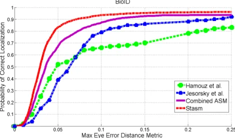
Figure 2.8: Comparison of the proposed Combined-ASM with already published results for eyes detections on the BioID database.

(41)

related to the deye measurements including results of Jesorsky et al. [34], Hamouz et al. [30], and the results of the STASM software by Milborrow [44]. These results are compared with our Combined ASM model implementation. The first two methods are image-based methods, while the last two ones are structure-based methods. It is obvious that structure-based methods have better performance than image-based methods even at the error level of Error < 0.1. Our Combined ASM method performs better then the two image-based methods, but worse then the available STASM software.

The results of the STASM software that we trained with a different training data (the IMM database) are presented in Table2.1. Using different training database results in different results the for Stasm Software.The XM2VTS database contains more training images and more landmarks, this results in better detection performance. How-ever if we use same training database, the proposed C-ASM gives better results, see Table2.1.

Table 2.1: Evaluation results on the BioID Database. Spatial error rate (at 10 % ) of eyes and mouth centers detection, of various landmark detection algorithms on the BioID database [34](in %).

Method Result Training Database

Stasm-original 95 XM2VTS

Stasm-modify 78.5 IMM

SIFT-ASM 75 IMM

Combined-ASM 86 IMM

Evaluation on the FRGCv2.0 Database

From the FRGCv2.0 database [51], we used the subpart called spring2003 which contains 11, 204 images, to evaluate our landmark location precision. There are not published results available on the FRGCv2.0 related to landmark location. Therefore we can only compare our results with the results of the Stasm software.

Because with the Stasm software (that also uses a face detection part as a fist step) there are about 39 % of the above mentioned spring2003 set of the FRGCV2.0 database images where the STASM face detection algorithm fails, we applied our land-mark location software on the same set, for sake of comparison.

(42)

2.5. EXPERIMENTS FOR C-ASM LANDMARK LOCATION PRECISION EVALUATION 25 0 0.05 0.1 0.15 0.2 0.25 0 0.1 0.2 0.3 0.4 0.5 0.6 0.7 0.8 0.9 1

Probability of Correct Localization

FRGC V2.0

Max Eye Error Distance Metric

SIFT−ASM Stasm Combined−ASM 0 0.05 0.1 0.15 0.2 0.25 0 0.1 0.2 0.3 0.4 0.5 0.6 0.7 0.8 0.9 1

Mouth Error Distance Metric

Probability of Correct Localization

FRGC V2.0

Combined−ASM SIFT−ASM Stasm

Figure 2.9: Cumulative histograms on FRGCv2.0 database with maximum eyes and mouth error, the Stasm in this experiential we used the default training data (STASM-original).

(43)

Combined ASM. In order to evaluate the contribution of using different features for different parts of the face, we also report results of using the ASM model with the SIFT features instead of the originally proposed grey level profile features (denoted as SIFT-ASM). The result show that the C-ASM method gives better performance for the eyes and mouth locations then the Stasm software and the ASM method with new SIFT features.

The C-ASM highly improves the precision of the mouth center, because the SIFT feature descriptor works more inaccurately in the contour points, and those points will affect the mouth region landmarks during the location phase. The results of the STASM software that we trained with a different training data (the IMM database) are presented in Table2.2. Using different training database also results in different results the for Stasm Software in this experiment. But the C-ASM got 95% correctly detected rate, using the IMM database for training.

Table 2.2: Evaluation results on the FRGCv2.0 Database. Spatial error rate (at 10 %) of eyes and mouth centers detection, of various landmark detection algorithms on the FRGCv2.0 Database [51].

Method Result Database Stasm-original 81.6 XM2VTS

Stasm-modify 77.4 IMM

SIFT-ASM 86.8 IMM

Combined-ASM 95 IMM

In this experiment, we only measure the landmark location precision on the FRGCv2.0 database by comparing the detected landmarks and the ground truth. We will study the influence of the landmarks location for face verification on the MBGCv1.0 and v2.0 databases, where no manually annotated landmarks are provided.

2.5.3 Experimental Discussion

The above presented experiments show that structure-based methods have bet-ter performance than image-based methods for facial landmark location. The Stasm software which uses the 2D profile and an extended set of landmarks for the training phase, presents better results on the BioID database compared to the C-ASM. But it is not as good as the proposed C-ASM for the FRGCv2.0 Database.

(44)

2.6. APPLICATION FOR 2D FACE RECOGNITION 27

One possible reason is due to the different characteristics of the databases. In the BioID database, all the images are captured when the person is near the camera, so the face is the largest part of the image. In the FRGCv2.0 database, there are uncontrolled images where the human face occupies a smaller area in the image. When the face area is small in the image, the initialization from the face detector will not be as precise as for ”passport style” photographs. Actually the ASM is an iteration strategy whose performance highly depends on the initialization. The Stasm software uses 2D profile as Local Texture Models which will increase the precision, while C-ASM use the SIFT descriptor which increase the robustness when bad initialization happens. Because the SIFT descriptor is scale and rotation invariant, even if the face area detected by the face detector is enlarged and decreased or distorted, it will not affect the Local Texture Models matching phase.

In the BioID database the average distance between two eyes is about fifty pixels, one pixel costs two percent error rate, and that error can be ignored when nor-malizing the face for face recognition. In that case the Combined-ASM algorithm seems to be robust without losing much of its accuracy for facial landmark detection for face recognition in cases when illumination, scale and small pose variation is present in the recording conditions (such as present in the FRGCv2). That is to say the proposed C-ASM is more suitable for uncontrolled images under degraded conditions, because the robustness of the SIFT descriptor and the separation in facial internal and facial contour region.

2.6 Application for 2D Face Recognition

As summarized in [1] by Zhao et al. in 2006, automated recognition of faces has reached a certain level of maturity, but technological challenges still exist in many aspects. For example, robust face recognition in outdoor-like environments is still dif-ficult. It is also important to precise that in a broader sense face recognition implies usually face detection, face normalization, feature extraction and face recognition tasks (modules). A lot of methods need facial landmark location for the normalization step. Therefore all those problems have to be solved separately in order to have good face recognition systems. In that case a robust and automatic facial landmark location