New Architectures for Handwritten Mathematical Expressions Recognition

HAL Id: tel-01754478

https://hal.archives-ouvertes.fr/tel-01754478

Submitted on 30 Mar 2018

HAL is a multi-disciplinary open access

archive for the deposit and dissemination of sci-entific research documents, whether they are pub-lished or not. The documents may come from teaching and research institutions in France or abroad, or from public or private research centers.

L’archive ouverte pluridisciplinaire HAL, est destinée au dépôt et à la diffusion de documents scientifiques de niveau recherche, publiés ou non, émanant des établissements d’enseignement et de recherche français ou étrangers, des laboratoires publics ou privés.

Expressions Recognition

Ting Zhang

To cite this version:

Ting Zhang. New Architectures for Handwritten Mathematical Expressions Recognition. Image Processing [eess.IV]. Université de nantes, 2017. English. �tel-01754478�

Ting Z

HANG

grade de Docteur de l’Université de Nantes

sous le sceau de l’Université Bretagne Loire

École doctorale : Sciences et technologies de l’information, et mathématiques Discipline : Informatique

Spécialité : Informatique et applications

Unité de recherche : Laboratoire des Sciences du Numérique de Nantes (LS2N) Soutenue le 26 Octobre 2017

New Architectures for Handwritten

Mathematical Expressions Recognition

JURY

Rapporteurs : Mme_{Laurence LIKFORMAN-SULEM, Maitre de conférences, HDR, Telecom ParisTech}

M. Thierry PAQUET, Professeur, Université de Rouen

Examinateur : M. Christophe GARCIA, Professeur, Institut National des Sciences Appliquées de Lyon

Directeur de thèse : M. Christian VIARD-GAUDIN, Professeur, Université de Nantes

Thanks to the various encounters and choices in life, I could have an experience studying in France at a fairly young age. Along the way, I met a lot of beautiful people and things.

Christian and Harold, you are so nice professors. This thesis would not have been possible without your considerate guidance, advice and encouragement. Thank you for sharing your knowledge and experience, for reading my papers and thesis over and over and providing meaningful comments. Your serious attitude towards work has a deep impact on me, today and tomorrow. Harold, thanks for your help in technique during the 3 years’ study. Thank all the colleagues from IVC/IRCCyN or IPI/LS2N for giving me such a nice working environment, for so many warm moments, for giving me help when I need some one to speak French to negotiate on the phone, many times. Suiyi and Zhaoxin, thanks for being rice friends with me each lunch in Polytech. Thanks all the friends I met in Nantes for so much laughing, so many colorful weekends with you. Also, I would like to thank the China Scholarship Council (CSC) for supporting 3 years’ PhD studentship at Université de Nantes. Finally, thank my parents, little brother and my grandparents for their understanding, support to my study, and endless love to me.

In addition, I would like to thank the members of the dissertation committee for accepting being either examiner or reviewer, and putting efforts on reviewing this thesis.

List of Tables 7

List of Figures 9

List of Abbreviations 13

1 Introduction 15

1.1 Motivation . . . 15

1.2 Mathematical expression recognition . . . 16

1.3 The proposed solution . . . 19

1.4 Thesis structure . . . 21

I

State of the art

23

2.1.1 Symbol level: Symbol relation (layout) tree . . . 25

2.1.2 Stroke level: Stroke label graph . . . 28

2.1.3 Performance evaluation with stroke label graph . . . 29

2.2 Mathematical expression recognition . . . 31

2.2.1 Overall review . . . 32

2.2.2 The recent integrated solutions . . . 33

2.2.3 End-to-end neural network based solutions . . . 37

2.2.4 Discussion . . . 37

3 Sequence labeling with recurrent neural networks 41 3.1 Sequence labeling . . . 41

3.2 Recurrent neural networks . . . 42

3.2.1 Topology . . . 42

3.2.2 Forward pass . . . 44

3.2.3 Backward pass . . . 44

3.2.4 Bidirectional networks . . . 45

3.3 Long short-term memory (LSTM) . . . 46

3.3.1 Topology . . . 46

3.3.2 Forward pass . . . 47

3.3.3 Backward pass . . . 48

3.3.4 Variants . . . 49

3.4 Connectionist temporal classification (CTC) . . . 51

3.4.1 From outputs to labelings . . . 51

3.4.2 Forward-backward algorithm . . . 51 3

3.4.3 Loss function . . . 53

3.4.4 Decoding . . . 54

II

Contributions

57

4.1.1 Complexity of expressions . . . 60

4.1.2 The proposed idea . . . 60

4.2 Detailed Implementation . . . 62

4.2.1 BLSTM Inputs . . . 63

4.2.2 Features . . . 63

4.2.3 Training process — local connectionist temporal classification . . . 64

4.2.4 Recognition Strategies . . . 67

4.3 Experiments . . . 68

4.3.1 Data sets . . . 69

4.3.2 Experiment 1: theoretical evaluation . . . 69

4.3.3 Experiment 2 . . . 71

4.3.4 Experiment 3 . . . 74

4.4 Discussion . . . 74

5 Mathematical expression recognition by merging multiple paths 77 5.1 Overview of graph representation . . . 77

5.2 The framework . . . 80

5.3 Detailed implementation . . . 81

5.3.1 Derivation of an intermediate graph G . . . 81

5.3.2 Graph evaluation . . . 82

5.3.3 Select paths from G . . . 84

5.3.4 Training process . . . 85

5.3.5 Recognition . . . 85

5.3.6 Merge paths . . . 85

5.4 Experiments . . . 87

5.5 Discussion . . . 92

6 Mathematical expression recognition by merging multiple trees 93 6.1 Overview: Non-chain-structured LSTM . . . 93

6.2 The proposed Tree-based BLSTM . . . 94

6.3 The framework . . . 97

6.4 Tree-based BLSTM for online mathematical expression recognition . . . 97

6.4.1 Derivation of an intermediate graph G . . . 97

6.4.2 Graph evaluation . . . 101

6.4.3 Derivation of trees from G . . . 101

6.4.4 Feed the inputs of the Tree-based BLSTM . . . 103

6.4.5 Training process . . . 104 6.4.6 Recognition process . . . 108 6.4.7 Post process . . . 108 6.5 Experiments . . . 109 6.5.1 Experiment 1 . . . 109 6.5.2 Experiment 2 . . . 110 6.5.3 Experiment 3 . . . 113

6.6 Error analysis . . . 115

6.7 Discussion . . . 116

7 Conclusion and future works 123 7.1 Conclusion . . . 123

7.2 Future works . . . 125

8 Résumé étendu en français 127 8.1 Introduction . . . 127

8.2 Etat de l’art . . . 128

8.2.1 Représentation des EM . . . 128

8.2.2 Réseaux Long Short-Term Memory . . . 128

8.2.3 La couche CTC : Connectionist temporal classification . . . 130

8.3 Reconnaissance par un unique chemin . . . 130

8.4 Reconnaissance d’EM par fusion de chemins multiples . . . 131

8.5 Reconnaissance d’EM par fusion d’arbres . . . 132

Bibliography 135

2.1 Illustration of the terminology related to recall and precision. . . 31 4.1 The symbol level evaluation results on CROHME 2014 test set (provided the ground truth

labels on the time path). . . 71 4.2 The expression level evaluation results on CROHME 2014 test set (provided the ground

truth labels on the time path). . . 71 4.3 The symbol level evaluation results on CROHME 2014 test set, including the experiment

results in this work and CROHME 2014 participant results. . . 72 4.4 The expression level evaluation results on CROHME 2014 test set, including the experiment

results in this work and CROHME 2014 participant results. . . 72 4.5 The symbol level evaluation results (mean values) on CROHME 2014 test set with different

training and decoding methods, features. . . 74 4.6 The standard derivations of the symbol level evaluation results on CROHME 2014 test set

with local CTC training and maximum decoding method, 5 local features. . . 74 5.1 The symbol level evaluation results on CROHME 2014 test set (provided the ground truth

labels of the nodes and edges of the built graph). . . 84 5.2 The expression level evaluation results on CROHME 2014 test set (provided the ground

truth labels of the nodes and edges of the built graph). . . 84 5.3 Illustration of the used classifiers in the different experiments depending of the type of path. 87 5.4 The symbol level evaluation results on CROHME 2014 test set, including the experiment

results in this work and CROHME 2014 participant results. . . 88 5.5 The expression level evaluation results on CROHME 2014 test set, including the experiment

results in this work and CROHME 2014 participant results . . . 89 6.1 The symbol level evaluation results on CROHME 2014 test set (provided the ground truth

labels). . . 101 6.2 The expression level evaluation results on CROHME 2014 test set (provided the ground

truth labels). . . 101 6.3 The different types of the derived trees. . . 103 6.4 The symbol level evaluation results on CROHME 2014 test set with Tree-Time only. . . . 110 6.5 The expression level evaluation results on CROHME 2014 test set with Tree-Time only. . 110 6.6 The symbol level evaluation results on CROHME 2014 test set with 3 trees, along with

CROHME 2014 participant results. . . 111 6.7 The expression level evaluation results on CROHME 2014 test set with 3 trees, along with

CROHME 2014 participant results. . . 112 6.8 The symbol level evaluation results on CROHME 2016 test set with the system of Merge 9,

along with CROHME 2016 participant results. . . 113 6.9 The expression level evaluation results on CROHME 2016 test set with the system of Merge

9, along with CROHME 2016 participant results. . . 113 6.10 The symbol level evaluation results on CROHME 2014 test set with 11 trees. . . 114

6.11 The expression level evaluation results on CROHME 2014 test set with 11 trees. . . 114 6.12 Illustration of node (SLG) label errors of (Merge 9 ) on CROHME 2014 test set. We only

list the cases that occur ≥ 10 times. . . 115 6.13 Illustration of edge (SLG) label errors of (Merge 9 ) on CROHME 2014 test set. . . 116 8.1 Les résultats au niveau symbole sur la base de test de CROHME 2014, comparant ces

travaux et les participants à la compétition. . . 133 8.2 Les résultats au niveau expression sur la base de test CROHME 2014, comparant ces travaux

1.1 Illustration of mathematical expression examples. (a) A simple and liner expression con-sisting of only left-right relationship. (b) A 2-D expression where left-right, above-below,

superscript relationships are involved. . . 16

1.2 Illustration of expression zd_{+ z written with 5 strokes. . . . 17}

1.3 Illustration of the symbol segmentation of expression zd+ z written with 5 strokes. . . 17

1.4 Illustration of the symbol recognition of expression zd+ z written with 5 strokes. . . 18

1.5 Illustration of the structural analysis of expression zd_{+ z written with 5 strokes. Sup :} Superscript, R : Right. . . 18

1.6 Illustration of the symbol relation tree of expression zd+ z. Sup : Superscript, R : Right. 18 1.7 Introduction of traits "in the air" . . . 19

1.8 Illustration of the proposal of recognizing ME expressions with a single path. . . 20

1.9 Illustration of the proposal of recognizing ME expressions by merging multiple paths. . . . 21

1.10 Illustration of the proposal of recognizing ME expressions by merging multiple trees. . . . 22

2.1 Symbol relation tree (a) and operator tree (b) of expression (a+b)2. Sup : Superscript, R : Right, Arg : Argument. . . 26

2.2 The symbol relation tree (SRT) for (a) a+b_c , (b) a + b_c. ’R’ refers to Right relationship. . . 26

2.3 The symbol relation trees (SRT) for (a) √3 _{x, (b)} n P i=0 xi _{and (c)} R xxdx. ’R’ refers to Right relationship while ’Sup’ and ’Sub’ denote Superscript and Subscript respectively. . . 27

2.4 Math file encoding for expression (a + b)2_{. (a) Presentation MathML; (b) LA} TEX. Adapted from [Zanibbi and Blostein, 2012]. . . 27

2.5 (a) 2 + 2 written with four strokes; (b) the symbol relation tree of 2 + 2; (c) the SLG of 2 + 2. The four strokes are indicated as s1, s2, s3, s4 in writing order. ’R’ is for left-right relationship . . . 28

2.6 The file formats for representing SLG considering the expression in Figure2.5a. (a) The file format taking stroke as the basic entity. (b) The file format taking symbol as the basic entity. 29 2.7 Adjacency Matrices for Stroke Label Graph. (a) The adjacency matrix format: li denotes the label of stroke si and eij is the label of the edge from stroke si to stroke sj. (b) The adjacency matrix of labels corresponding to the SLG in Figure 2.5c. . . 30

2.8 ’2 + 2’ written with four strokes was recognized as ’2 − 12’. (a) The SLG of the recognition result; (b) the corresponding adjacency matrix. ’Sup’ denotes Superscript relationship. . . 30

2.9 Example of a search for most likely expression candidate using the CYK algorithm. Ex-tracted from [Yamamoto et al., 2006]. . . 33

2.10 The system architecture proposed in [Awal et al., 2014]. Extracted from [Awal et al., 2014]. 34 2.11 A simple example of Fuzzy r-CFG. Extracted from [MacLean and Labahn, 2013]. . . 35

2.12 (a) An input handwritten expression; (b) a shared parse forest of (a) considering the gram-mar depicted in Figure 2.11. Extracted from [MacLean and Labahn, 2013] . . . 36

2.13 Geometric features for classifying the spatial relationship between regions B and C. Ex-tracted from [Álvaro et al., 2016] . . . 37

2.14 Achitecture of the recognition system proposed in [Julca-Aguilar, 2016]. Extracted from

[Julca-Aguilar, 2016] . . . 38

2.15 Network architecture of WYGIWYS. Extracted from [Deng et al., 2016] . . . 39

3.1 Illustration of sequence labeling task with the examples of handwriting (top) and speech (bottom) recognition. Input signals is shown on the left side while the ground truth is on the right. Extracted from [Graves et al., 2012]. . . 42

3.2 A multilayer perceptron. . . 43

3.3 A recurrent neural network. The recurrent connections are highlighted with red color. . . . 43

3.4 An unfolded recurrent network. . . 43

3.5 An unfolded bidirectional network. Extracted from [Graves et al., 2012]. . . 46

3.6 LSTM memory block with one cell. Extracted from [Graves et al., 2012]. . . 47

3.7 A deep bidirectional LSTM network with two hidden levels. . . 50

3.8 (a) A chain-structured LSTM network; (b) A tree-structured LSTM network with arbitrary branching factor. Extracted from [Tai et al., 2015]. . . 50

3.9 Illustration of CTC forward algorithm. Blanks are represented with black circles and labels are white circles. Arrows indicate allowed transitions. Adapted from [Graves et al., 2012]. 52 3.10 Mistake incurred by best path decoding. Extracted from [Graves et al., 2012]. . . 55

3.11 Prefix search decoding on the alphabet {X, Y}. Extracted from [Graves et al., 2012]. . . . 55

4.1 Illustration of the proposal that uses BLSTM to interpret 2-D handwritten ME. . . 59

4.2 Illustration of the complexity of math expressions. . . 60

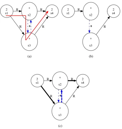
4.3 (a) The time path (red) in SLG; (b) the SLG obtained by using the time path; (c) the post-processed SLG of ’2 + 2’, added edges are depicted as bold. . . 61

4.4 (a) Peowritten with four strokes; (b) the SRT of Peo; (c) r2h written with three strokes; (d) the SRT of r2_{h, the red edge cannot be generated by the time sequence of strokes . . . . . 62}

4.5 The illustration of on-paper points (blue) and in-air points (red) in time path, a1+a2written with 6 strokes. . . 63

4.6 The illustration of (a) θi, φi and (b) ψi used in feature description. The points related to feature computation at piare depicted in red. . . 64

4.7 The possible sequences of point labels in one stroke. . . 65

4.8 Local CTC forward-backward algorithm. Black circles represent labels and white circles represent blanks. Arrows signify allowed transitions. Forward variables are updated in the direction of the arrows, and backward variables are updated in the reverse direction. . . 66

4.9 Illustration for the decision of the label of strokes. As stroke 5 and 7 have the same label, the label of stroke 6 could be ’+’, ’_’ or one of the six relationships. All the other strokes are provided with the ground truth labels in this example. . . 68

4.10 Real examples from CROHME 2014 data set. (a) sample from Data set 1; (b) sample from Data set 2; (c) sample from Data set 3. . . 70

4.11 (a) a ≥ b written with four strokes; (b) the built SLG of a ≥ b according to the recognition result, all labels are correct. . . 73

4.12 (a) 44 −4₄ written with six strokes; (b) the ground-truth SLG; (c) the rebuilt SLG according to the recognition result. Three edge errors occurred: the Right relation between stroke 2 and 4 was missed because there is no edge from stroke 2 to 4 in the time path; the edge from stroke 4 to 3 was missed for the same reason; the edge from stroke 2 to 3 was wrongly recognized and it should be labeled as N oRelation. . . 73

5.1 Examples of graph models. (a) An example of minimum spanning tree at stroke level. Extracted from [Matsakis, 1999]. (b) An example of Delaunay-triangulation-based graph at symbol level. Extracted from [Hirata and Honda, 2011]. . . 78

5.3 Stroke representation. (a) The bounding box. (b) The convex hull. . . 79

5.4 Illustration of the proposal that uses BLSTM to interpret 2-D handwritten ME. . . 80

5.5 Illustration of visibility between a pair of strokes. s1 and s3 are visible to each other. . . . 81

5.6 Five directions for a stroke si. Point (0, 0) is the center of bounding box of si. The angle of each region is π₄. . . 82

5.7 (a)_dxdax is written with 8 strokes; (b) the SLG built from raw input using the proposed method; (c) the SLG from ground truth; (d) illustration of the difference between the built graph and the ground truth graph, red edges denote the unnecessary edges and blue edges refer to the missed ones compared to the ground truth. . . 83

5.8 Illustration of the strategy for merge. . . 86

5.9 (a) a ≥ b written with four strokes; (b) the derived graph from the raw input; (c) the labeled graph (provided the label and the related probability) with merging 7 paths; (d) the built SLG after post process, all labels are correct. . . 90

5.10 (a) 44 − 4₄ written with six strokes; (b) the derived graph; (c) the built SLG by merging several paths; (d) the built SLG with N oRelation edges removed. . . 91

6.1 (a) A chain-structured LSTM network; (b) A tree-structured LSTM network with arbitrary branching factor. Extracted from [Tai et al., 2015]. . . 94

6.2 A tree based structure for chains (from root to leaves). . . 94

6.3 A tree based structure for chains (from leaves to root). . . 95

6.4 Illustration of the proposal that uses BLSTM to interpret 2-D handwritten ME. . . 97

6.5 Illustration of visibility between a pair of strokes. s1 and s3 are visible to each other. . . . 98

6.6 Five regions for a stroke si. Point (0, 0) is the center of bounding box of si. The angle range of R1 region is [−π₈,π₈]; R2 : [π₈,3∗π₈ ]; R3 : [3∗π₈ ,7∗π₈ ]; R4 : [−7∗π₈ , −3∗π₈ ]; R5 : [−3∗π₈ , −π₈]. 98 6.7 (a)f_a = _fb is written with 10 strokes; (b) create nodes; (c) add Crossing edges. C : Crossing. 99 6.7 (d) add R1, R2, R3, R4, R5 edges; (e) add T ime edges. C : Crossing, T : T ime. . . 100

6.8 (a) f_a = _fb is written with 10 strokes; (b) the derived graph G, the red part is one of the possible trees with s2 as the root. C : Crossing, T : T ime. . . 102

6.9 A re-sampled tree. The small arrows between points provide the directions of information flows. With regard to the sequence of points inside one node or edge, most of small arrows are omitted. . . 103

6.10 A tree-based BLSTM network with one hidden level. We only draw the full connection on one short sequence (red) for a clear view. . . 104

6.11 Illustration for the pre-computation stage of tree-based BLSTM. (a) From the input layer to the hidden layer (from root to leaves), (b) from the input layer to the hidden layer (from leaves to root). . . 106

6.12 The possible labels of points in one short sequence. . . 106

6.13 CTC forward-backward algorithm in one stroke Xi. Black circle represents label liand white circle represents blank. Arrows signify allowed transitions. Forward variables are updated in the direction of the arrows, and backward variables are updated in the reverse direction. This figure is a local part (limited in one stroke) of Figure 4.8. . . 107

6.14 Possible relationship conflicts existing in merging results. . . 109

6.15 (a) a ≥ b written with four strokes; (b) the derived graph; (b) Tree-Time; (c)Tree-Left-R1 (In this case, Tree-0-R1 is the same as Tree-Left-R1 ); (e) the built SLG of a ≥ b after merging several trees and performing other post process steps, all labels are correct; (f) the built SLG with N oRelation edges removed. . . 117

6.16 (a) 44 − 4₄ written with six strokes; (b) the derived graph; (b) Tree-Time; (c)Tree-Left-R1 (In this case, Tree-0-R1 is the same as Tree-Left-R1 ); . . . 118

6.16 (b)the built SLG after merging several trees and performing other post process steps; (c) the built SLG with N oRelation edges removed. . . 119

6.17 (a) ₉₊9√

9 written with 7 strokes; (b) the derived graph; (b) Tree-Time; . . . 120

6.17 (d)Tree-Left-R1 ; (e)Tree-0-R1 ; (f)the built SLG after merging several trees and performing other post process steps; (g) the built SLG with N oRelation edges removed. There is a node label error: the stroke 2 with the ground truth label ’9’ was wrongly classified as ’→’. 121 8.1 L’arbre des relations entre symboles (SRT) pour (a) a+b_c et (b) a + b_c,‘R’définit une relation à droite. . . 128

8.2 (a) « 2 + 2 » écrit en quatre traits ; (b) le graphe SLG de « 2 + 2 ». Les quatre traits sont repérés s1, s2, s3 et s4, respectant l’ordre chronologique. (ver.) et (hor.) ont été ajoutés pour distinguer le trait horizontal et vertical du ‘+’. ‘R’ représente la relation Droite. . . . 129

8.3 Un réseau récurrent monodirectionnel déplié. . . 129

8.4 Illustration de la méthode basée sur un seul chemin. . . 130

8.5 Introduction des traits « en l’air ». . . 131

8.6 Reconnaissance par fusion de chemins. . . 131

2D-PCFGs Two-Dimensional Probabilistic Context-Free Grammars. AC Averaged Center.

ANNs Artificial Neural Networks. BAR Block Angle Range.

BB Bounding Box.

BBC Bounding Box Center.

BLSTM Bidirectional Long Short-Term Memory. BP Back Propagation.

BPTT Back Propagation Through Time.

BRNNs Bidirectional Recurrent Neural Networks (BRNNs). CH Convex Hull.

CNN Convolutional Neural Network. CPP Closest Point Pair.

CROHME Competition on Recognition of Handwritten Mathematical Expressions. CTC Connectionist Temporal Classification.

CYK Cock Younger Kasami. DT Delaunay Triangulation.

FNNs Feed-forward Neural Networks. HMM Hidden Markov Model.

KNN K Nearest Neighbor. LOS Line Of Sight.

ME Mathematical Expression. MLP Multilayer Perceptron. MST Minimum Spanning Tree.

r-CFG Relational Context-Free Grammar. RNN Recurrent Neural Network.

RTRL Real Time Recurrent Learning. SLG Stroke Label Graph.

SRT Symbol Relation Tree. TS Time Series.

UAR Unblocked Angle Range. VAR Visibility Angle Range.

1

Introduction

In this thesis, we explore the idea of online handwritten Mathematical Expression (ME) interpretation using Bidirectional Long Short-Term Memory (BLSTM) and Connectionist Temporal Classification (CTC) topology, and finally build a graph-driven recognition system, bypassing the high time complexity and manual work with the classical grammar-driven systems. Advanced recurrent neural network BLSTM with a CTC output layer achieved great success in sequence labeling tasks, such as text and speech recognition. However, the move from sequence recognition to mathematical expression recognition is far from being straightforward. Unlike text or speech where only left-right (or past-future) relationship is involved, ME has a 2 dimensional (2-D) structure consisting of relationships like subscript and superscript. To solve this recognition problem, we propose a graph-driven system, extending the chain-structured BLSTM to a tree structure topology allowing to handle the 2-D structure of ME, and extending CTC to local CTC to relatively constrain the outputs.

In the first section of the this chapter, we introduce the motivation of our work from both the research point and the practical application point. Section 1.2 provides a global view of the mathematical expression recognition problem, covering some basic concepts and the challenges involved in it. Then in Section 1.3, we describe the proposed solution concisely, to offer the readers an overall view of main contributions of this work. The thesis structure will be presented in the end of the chapter.

1.1

Motivation

A visual language is defined as any form of communication that relies on two- or three-dimensional graphics rather than simply (relatively) linear text [Kremer, 1998]. Mathematical expressions, plans and musical notations are commonly used cases in visual languages [Marriott et al., 1998]. As an intuitive and easily (relatively) comprehensible knowledge representation model, mathematical expression (Figure 1.1) could help the dissemination of knowledge in some related domains and therefore is essential in scientific documents. Currently, common ways to input mathematical expressions into electronic devices include typesetting systems such as LA_{TEX and mathematical editors such as the one embedded in MS-Word. But}

these ways require that users could hold a large number of codes and syntactic rules, or handle the trou-blesome manipulations with keyboards and mouses as interface. As another option, being able to input mathematical expressions by hand with a pen tablet, as we write them on paper, is a more efficient and direct mean to help the preparation of scientific document. Thus, there comes the problem of handwritten mathematical expression recognition. Incidentally, the recent large developments of touch screen devices also drive the research of this field.

(a)

(b)

Figure 1.1 – Illustration of mathematical expression examples. (a) A simple and liner expression consisting of only left-right relationship. (b) A 2-D expression where left-right, above-below, superscript relationships are involved.

Handwritten mathematical expression recognition is an appealing topic in pattern recognition field since it exhibits a big research challenge and underpins many practical applications. From a scientific point of view, a large set of symbols (more than 100) needs to be recognized, and also the 2 dimensional (2-D) struc-tures (specifically the relationships between a pair of symbols, for example superscript and subscript), both of which increase the difficulty of this recognition problem. With regard to the application, it offers an easy and direct way to input MEs into computers, and therefore improves productivity for scientific writers. Research on the recognition of math notation began in the 1960’s [Anderson, 1967], and several re-search publications are available in the following thirty years [Chang, 1970, Martin, 1971, Anderson, 1977]. Since the 90’s, with the large developments of touch screen devices, this field has started to be active, gaining amounts of research achievement and considerable attention from the research community. A number of surveys [Blostein and Grbavec, 1997, Chan and Yeung, 2000, Tapia and Rojas, 2007, Zanibbi and Blostein, 2012] summarize the proposed techniques for math notation recognition. This research domain has been boosted by the Competition on Recognition of Handwritten Mathematical Expressions (CROHME) [Mouchère et al., 2016], which began as part of the International Conference on Document Analysis and Recognition (ICDAR) in 2011. It provides a platform for researchers to test their methods and compare them, and then facilitate the progress in this field. It attracts increasing participation of research groups from all over the world. In this thesis, the provided data and evaluation tools from CROHME will be used and results will be compared to participants.

1.2

Mathematical expression recognition

We usually divide handwritten MEs into online and offline domains. In the offline domain, data is available as an image, while in the online domain it is a sequence of strokes, which are themselves sequences of points recorded along the pen trajectory. Compared to the offline ME, time information is available in online form. This thesis will be focused on online handwritten ME recognition.

For the online case, a handwritten mathematical expression could have one or more strokes and a stroke is a sequence of points sampled from the trajectory of the writing tool between a pen-down and a pen-up at a fixed interval of time. For example, the expression zd+ z shown in Figure 1.2 is written with 5 strokes, two strokes of which belong to the symbol ‘+‘.

Generally, ME recognition involves three tasks [Zanibbi and Blostein, 2012]:

(1) Symbol Segmentation, which consists in grouping strokes that belong to the same symbol. In Figure 1.3, we illustrate the segmentation of the expression zd+ z where stroke3 and stroke4 are grouped as a

Figure 1.2 – Illustration of expression zd+ z written with 5 strokes.

Figure 1.3 – Illustration of the symbol segmentation of expression zd_{+ z written with 5 strokes.}

symbol candidate. This task becomes very difficult in the presence of delayed strokes, which occurs when interspersed symbols are written. For example, it could be possible in the real case that someone write first a part of the symbol ‘+‘ (stroke3), and then the symbol ‘z‘ (stroke5), in the end complete the other part of the symbol ‘+‘ (stroke4). Thus, in fact any combination of any number of strokes could form a symbol candidate. It is exhausting to take into account each possible combination of strokes, especially for complex expressions having a large number of strokes.

(2) Symbol Recognition, the task of labeling the symbol candidates to assign each of them a symbol class. Still considering the same sample zd+ z, Figure 1.4 presents the symbol recognition of it. This is as well a difficult task because the number of classes is quite important, more than one hundred different symbols including digits, alphabet, operators, Greek letters and some special math symbols; it exists an overlapping between some symbol classes: (1) for instance, digit ‘0’, Greek letter ‘θ’, and character ‘O’ might look about the same when considering different handwritten samples (inter-class variability); (2) there is a large intra-class variability because each writer has his own writing style. Being an example of inter-class vari-ability, the stroke5 in Figure 1.4 looks like and could be recognized as ‘z’, ‘Z’ or ‘2’. To address these issues, it is important to design robust and efficient classifiers as well as a large training data set. Nowadays, most of the proposed solutions are based on machine learning algorithms such as neural networks or support vector machines.

(3) Structural Analysis, its goal is to identify spatial relations between symbols and with the help of a 2-D language to produce a mathematical interpretation, such as a symbol relation tree which will be emphasized in later chapter. For instance, the Superscript relationship between the first ‘z’ and ‘d’, and the Right relationship between the first ‘z’ and ‘+’ as illustrated in Figure 1.5. Figure 1.6 provides the corresponding symbol relation tree which is one of the possible ways to represent math expressions. Structural analysis strongly depends on the correct understanding of relative positions among symbols. Most approaches con-sider only local information (such as relative symbol positions and their sizes) to determine the relation between a pair of symbols. Although some approaches have proposed the use of contextual information to improve system performances, modeling and using such information is still challenging.

These three tasks can be solved sequentially or jointly. In the early stages of the study, most of the proposed solutions [Chou, 1989, Koschinski et al., 1995, Winkler et al., 1995, Matsakis, 1999, Zanibbi et al., 2002, Tapia and Rojas, 2003, Tapia, 2005, Zhang et al., 2005] are sequential ones which treat the

Figure 1.4 – Illustration of the symbol recognition of expression zd+ z written with 5 strokes.

Figure 1.5 – Illustration of the structural analysis of expression zd + z written with 5 strokes. Sup : Superscript, R : Right.

z + z

d

R R

Sup

recognition problem as a two-step pipeline process, first symbol segmentation and classification, and then structural analysis. The task of structural analysis is performed on the basis of the symbol segmentation and classification result. The main drawback of these sequential methods is that the errors from symbol segmentation and classification will be propagated to structural analysis. In other words, symbol recog-nition and structural analysis are assumed as independent tasks in the sequential solutions. However, this assumption conflicts with the real case in which these three tasks are highly interdependent by nature. For instance, human beings recognize symbols with the help of global structure, and vice versa.

The recent proposed solutions, considering the natural relationship between the three tasks, perform the task of segmentation at the same time build the expression structure: a set of symbol hypotheses maybe gen-erated and a structural analysis algorithm may select the best hypotheses while building the structure. The integrated solutions use contextual information (syntactic knowledge) to guide segmentation or recognition, preventing from producing invalid expressions like [a + b). These approaches take into account contextual information generally with grammar (string grammar [Yamamoto et al., 2006, Awal et al., 2014, Álvaro et al., 2014b, 2016, MacLean and Labahn, 2013] and graph grammar [Celik and Yanikoglu, 2011, Julca-Aguilar, 2016]) parsing techniques, producing expressions conforming to the rules of a manually defined grammar. Either string or graph grammar parsing, each one has a high computational complexity.

In conclusion, generally the current state of the art systems are grammar-driven solutions. For these grammar-driven solutions, it requires not only a large amount of manual work for defining grammars, but also a high computational complexity for grammar parsing process. As an alternative approach, we propose to explore a non grammar-driven solution for recognizing math expression. This is the main goal of this thesis, we would like to propose new architectures for mathematical expression recognition with the idea of taking advantage of the recent advances in recurrent neural networks.

1.3

The proposed solution

As well known, Bidirectional Long Short-term Memory (BLSTM) network with a Connectionist Tem-poral Classification (CTC) output layer achieved great success in sequence labeling tasks, such as text and speech recognition. This success is due to the LSTM’s ability of capturing long-term dependency in a sequence and the effectiveness of CTC training method. Unlike the grammdriven solutions, the new ar-chitectures proposed in this thesis include contextual information with BLSTM instead of grammar parsing technique. In this thesis, we will explore the idea of using the sequence-structured BLSTM with a CTC stage to recognize 2-D handwritten mathematical expression.

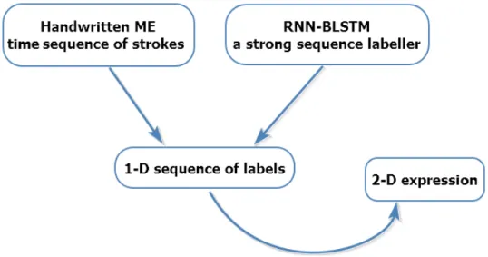
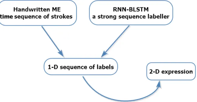
Mathematical expression recognition with a single path. As a first step to try, we consider linking the last point and the first point of a pair of strokes successive in the input time to allow the handwritten ME to be handled with BLSTM topology. As shown in Figure 1.7, after processing, the original 5 visible strokes

Figure 1.7 – Introduction of traits "in the air"

turn out to be 9 strokes; in fact, they could be regarded as a global sequence, just as same as the regular 1-D text. We would like to use these later added strokes to represent the relationships between pairs of stokes by assigning them a ground truth label. The remaining work is to train a model using this global sequence with

a BLSTM and CTC topology, and then label each stroke in the global sequence. Finally, with the sequence of outputted labels, we explore how to build a 2-D expression. The framework is illustrated in Figure 1.8.

Figure 1.8 – Illustration of the proposal of recognizing ME expressions with a single path.

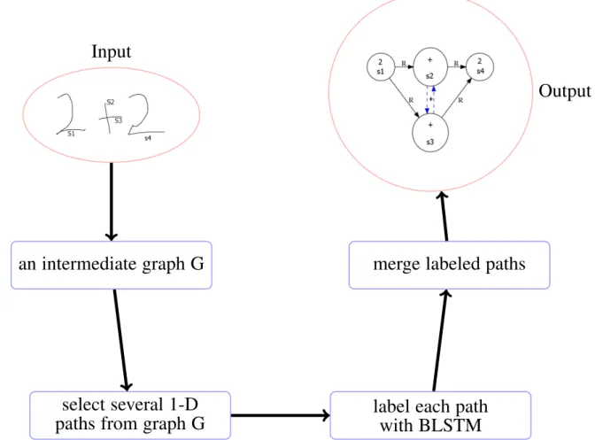
Mathematical expression recognition by merging multiple paths. Obviously, the solution of linking only pairs of strokes successive in the input time could handle just some relatively simple expressions. For complex expressions, some relationships could be missed such as the Right relationship between stroke1 and stroke5 in Figure 1.7. Thus, we turn to a graph structure to model the relationships between strokes in mathematical expressions. We illustrate this new proposal in Figure 1.9. As shown, the input of the recognition system is an handwritten expression which is a sequence of strokes; the output is the stroke label graph which consists of the information about the label of each stroke and the relationships between stroke pairs. As the first step, we derive an intermediate graph from the raw input considering both the temporal and spatial information. In this graph, each node is a stroke and edges are added according to temporal or spatial properties between strokes. We assume that strokes which are close to each other in time and space have a high probability to be a symbol candidate. Secondly, several 1-D paths will be selected from the graph since the classifier model we are considering is a sequence labeller. Indeed, a classical BLSTM-RNN model is able to deal with only sequential structure data. Next, we use the BLSTM classifier to label the selected 1-D paths. This stage consists of two steps —— the training and recognition process. Finally, we merge these labeled paths to build a complete stroke label graph.

Mathematical expression recognition by merging multiple trees. Human beings interpret handwrit-ten math expression considering the global contextual information. However, in the current system, even though several paths from one expression are taken into account, each of them is considered individually. The classical BLSTM model could access information from past and future in a long range but the infor-mation outside the single sequence is of course not accessible to it. Thus, we would like to develop a neural network model which could handle directly a structure not limited to a chain. With this new neural network model, we could take into account the information in a tree instead of a single path at one time when dealing with one expression.

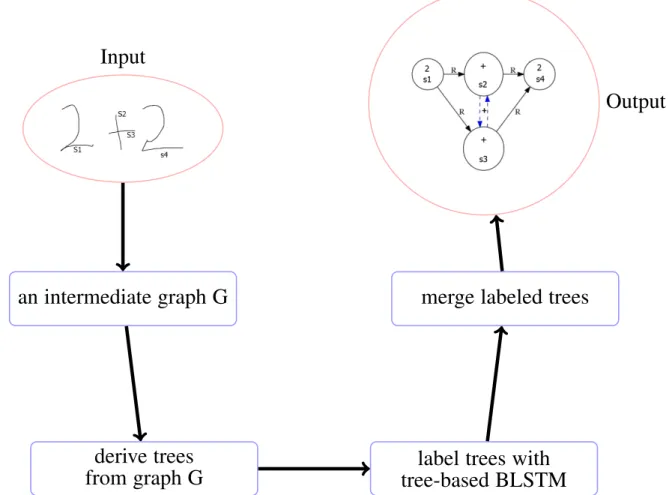
We extend the chain-structured BLSTM to tree structure topology and apply this new network model for online math expression recognition. Figure 1.10 provides a global view of the recognition system. Similar to the framework presented in Figure 1.9, we first drive an intermediate graph from the raw input. Then, instead of 1-D paths, we consider from the graph deriving trees which will be labeled by tree-based BLSTM model as a next step. In the end, these labeled trees will be merged to build a stroke label graph.

Input

Output

an intermediate graph G

merge labeled paths

select several 1-D

paths from graph G

label each path

_{with BLSTM}

Figure 1.9 – Illustration of the proposal of recognizing ME expressions by merging multiple paths.

1.4

Thesis structure

Chapter 2 describes the previous works on ME representation and recognition. With regards to repre-sentation, we introduce the symbol relation tree (symbol level) and the stroke label graph (stroke level). Furthermore, as an extension, we describe the performance evaluation based on stroke label graph. For ME recognition, we first review the entire history of this research subject, and then only focus on more recent solutions which are used for a comparison with the new architectures proposed in this thesis.

Chapter 3 is focused on sequence labeling using recurrent neural networks, which is the foundation of our work. First of all, we explain the concept of sequence labeling and the goal of this task shortly. Then, the next section introduces the classical structure of recurrent neural network. The property of this network is that it can memorize contextual information but the range of the information could be accessed is quite limited. Subsequently, long short-term memory is presented with the aim of overcoming the disadvantage of the classical recurrent neural network. The new architecture is provided with the ability of accessing information over long periods of time. Finally, we introduce how to apply recurrent neural network for the task of sequence labeling, including the existing problems and the solution to solve them, i.e. the connectionist temporal classification technology.

In Chapter 4, we explore the idea of recognizing ME expressions with a single path. Firstly, we globally introduce the proposal that builds stroke label graph from a sequence of labels, along with the existing limitations in this stage. Then, the entire process of generating the sequence of labels with BLSTM and local CTC given the input is presented in detail, including firstly feeding the inputs of BLSTM, then the training and recognition stages. Finally, the experiments and discussion are described. One main drawback of the strategy proposed in this chapter is that only stroke combinations in time series are used in the representation model. Thus, some relationships are missed at the modeling stage.

Input

Output

an intermediate graph G

merge labeled trees

derive trees

from graph G

_{tree-based BLSTM}

label trees with

Figure 1.10 – Illustration of the proposal of recognizing ME expressions by merging multiple trees. new model to overcome some limitations in the system of Chapter 4. The proposed solution will take into account more possible stroke combinations in both time and space such that less relationships will be missed at the modeling stage. We first provide an overview of graph representation related to build a graph from raw mathematical expression. Then we globally describe the framework of mathematical expression recognition by merging multiple paths. Next, all the steps of the recognition system are explained one by one in detail. Finally, the experiment part and the discussion part are presented respectively. One main limitation is that we use the classical chain-structured BLSTM to label a graph-structured input data.

In Chapter 6, we explore the idea of recognizing ME expressions by merging multiple trees, as a new model to overcome the limitation of the system of Chapter 5. We extend the chain-structured BLSTM to tree structure topology and apply this new network model for online math expression recognition. Firstly, a short overview with regards to the non-chain-structured LSTM is provided. Then, we present the new proposed neural network model named tree-based BLSTM. Next, the framework of ME recognition system based on tree-based BLSTM is globally introduced. Hereafter, we focus on the specific techniques involved in this system. Finally, experiments and discussion parts are covered respectively.

In Chapter 7, we conclude the main contributions of this thesis and give some thoughts about future work.

I

State of the art

2

Mathematical expression representation and

recognition

This chapter introduces the previous works regarding to ME representation and ME recognition. In the first part, we will review the different representation models on symbol and stroke level respectively. On symbol level, symbol relation (layout) tree is the one we mainly focus on; on stroke level, we will introduce stroke label graph which is a derivation of symbol relation tree. Note that stroke label graph is the final output form of our recognition system. As an extension, we also describe the performance evaluation based on stroke label graph. In the second part, we review first the history of this recognition problem, and then put emphasize on more recent solutions which are used for a comparison with the new architectures proposed in this thesis.

2.1

Mathematical expression representation

Structures can be depicted at three different levels: symbolic, object and primitive [Zanibbi et al., 2013]. In the case of handwritten ME, the corresponding levels are expression, symbol and stroke.

In this section, we will first introduce two representation models of math expression at the symbol level, especially Symbol Relation Tree (SRT). From the SRT, if going down to the stroke level, a Stroke Label Graph (SLG) could be derived, which is the current official model to represent the ground-truth of handwritten math expressions and also for the recognition outputs in Competitions CROHME.

2.1.1

Symbol level: Symbol relation (layout) tree

It is possible to describe a ME at the symbol level using a layout-based SRT, as well as an operator tree which is based on operator syntax. Symbol layout tree represents the placement of symbols on baselines (writing lines), and the spatial arrangement of the baselines [Zanibbi and Blostein, 2012]. As shown in Figure 2.1a, symbols ’(’, ’a’, ’+’, ’b’, ’)’ share a writing line while ’2’ belongs to the other writing line. An operator tree represents the operator and relation syntax for an expression [Zanibbi and Blostein, 2012]. The operator tree for (a + b)2shown in Figure 2.1b represents the addition of ’a’ and ’b’, squared. We will focus only on the model of symbol relation tree in the coming content since it is closely related to our work. In SRT, nodes represent symbols, while labels on the edges indicate the relationships between symbols. For example, in Figure 2.2a, the first symbol ’-’ on the base line is the root of the tree; the symbol ’a’ is Above ’-’ and the symbol ’c’ is Below ’-’. In Figure 2.2b, the symbol ’a’ is the root; the symbol ’+’ is on the

( a + b ) 2 R R R R Sup (a) EXP ADD 2 a b Arg1 Arg2 Arg1 Arg2 (b)

Figure 2.1 – Symbol relation tree (a) and operator tree (b) of expression (a + b)2_{. Sup : Superscript, R :}

Right, Arg : Argument.

Right of ’a’. As a matter of fact, the node inherits the spatial relationships of its ancestor. In Figure 2.2a, node ’+’ inherits the Above relationship of its ancestor ’a’. Thus, ’+’ is also Above ’-’ as ’a’. Similarly, ’b’ is on the Right of ’a’ and Above the ’-’. Note that all the inherited relationships are ignored when we depict the SRTs in this work. This will be also the case in the evaluation stage since knowing the original edges is enough to ensure a proper representation.

(a) (b)

Figure 2.2 – The symbol relation tree (SRT) for (a) a+b_c , (b) a + b_c. ’R’ refers to Right relationship.

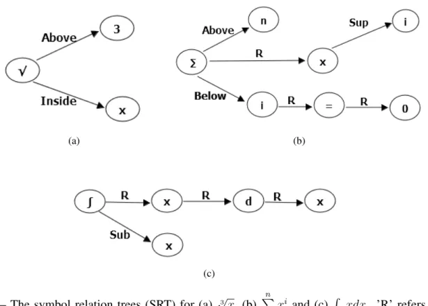
101 classes of symbols have been collected in CROHME data set, including digits, alphabets, operators and so on. Six spatial relationships are defined in the CROHME competition, they are: Right, Above, Below, Inside (for square root), Superscript, Subscript. For the case of nth-Roots, like√3_{x as illustrated} in Figure 2.3a, we define that the symbol ’3’ is Above the square root and ’x’ is Inside the square root. The limits of an integral and summation are designated as Above or Superscript and Below or Subscript depending on the actual position of the bounds. For example, in expression

n

P

i=0

ai_{, ’n’ is Above the ’P’ and}

’i’ is Below the ’P’ (Figure 2.3b). When we consider another case Pn_i=0ai_{, ’n’ is Superscript the ’P’}

and ’i’ is Subscript the ’P’. The same strategy is held for the limits of integral. As can be seen in Figure 2.3c, the first ’x’ is Subscript the ’R ’ in the expression R_xxdx.

(a) (b)

(c)

Figure 2.3 – The symbol relation trees (SRT) for (a) √3 _{x, (b)}

n

P

i=0

xi _{and (c)} R

xxdx. ’R’ refers to Right

relationship while ’Sup’ and ’Sub’ denote Superscript and Subscript respectively.

File formats for representing SRT

File formats for representing SRT include Presentation MathML1 _{and LA}

TEX, as shown in Figure 2.4. Compared to LA_{TEX, Presentation MathML contains additional tags to identify symbols types; these are}

primarily for formatting [Zanibbi and Blostein, 2012]. By the way, there are several files encoding for operator trees, including Content MathML and OpenMath [Davenport and Kohlhase, 2009, Dewar, 2000].

(a) (b)

Figure 2.4 – Math file encoding for expression (a + b)2_{. (a) Presentation MathML; (b) LA}

TEX. Adapted from [Zanibbi and Blostein, 2012].

2.1.2

Stroke level: Stroke label graph

SRT represents math expression at the symbol level. If we go down at the stroke level, a stroke label graph (SLG) can be derived from the SRT. In SLG, nodes represent strokes, while labels on the edges encode either segmentation information or symbol relationships. Relationships are defined at the level of symbols, implying that all strokes (nodes) belonging to one symbol have the same input and output edges. Consider the simple expression 2+2 written using four strokes (two strokes for ’+’) in Figure 2.5a. The corresponding SRT and SLG are shown in Figure 2.5b and Figure 2.5c respectively. As Figure 2.5c illustrates, nodes of SLG are labeled with the class of the corresponding symbol to which the stroke belongs. A dashed edge

(a) (b)

(c)

Figure 2.5 – (a) 2 + 2 written with four strokes; (b) the symbol relation tree of 2 + 2; (c) the SLG of 2 + 2. The four strokes are indicated as s1, s2, s3, s4 in writing order. ’R’ is for left-right relationship

corresponds to segmentation information; it indicates that a pair of strokes belongs to the same symbol. In this case, the edge label is the same as the common symbol label. On the other hand, the non-dashed edges define spatial relationships between nodes and are labeled with one of the different possible relationships between symbols. As a consequence, all strokes belonging to the same symbol are fully connected, nodes and edges sharing the same symbol label; when two symbols are in relation, all strokes from the source symbol are connected to all strokes from the target symbol by edges sharing the same relationship label.

Since CROHME 2013, SLG has been used to represent mathematical expressions [Mouchère et al., 2016]. As the official format to represent the ground-truth of handwritten math expressions and also for the recognition outputs, it allows detailed error analysis on stroke, symbol and expression levels. In order to be comparable to the ground truth SLG and allow error analysis on any level, our recognition system aims to generate SLG from the input. It means that we need a label decision for each stroke and each stroke pair used in a symbol relation.

File formats for representing SLG

The file format we are using for representing SLG is illustrated with the example 2 + 2 in Figure 2.6a. For each node, the format is like ’N, N odeIndex, N odeLabel, P robability’ where P robability is always 1 in ground truth and depends on the classifier in system output. When it comes to edges, the format will be ’E, F romN odeIndex, T oN odeIndex, EdgeLabel, P robability’.

An alternative format could be like the one shown in Figure 2.6b, which contains the same informa-tion as the previous one but with a more compact appearance. We take symbol as an individual to rep-resent in this compact version but include the stroke level information also. For each object (or symbol), the format is ’O, ObjectIndex, ObjectLabel, P robability, StrokeList’ in which StrokeList’ lists the in-dexes of the strokes this symbol consists of. Similarly, the representation for relationships is formatted as ’EO, F romObjectIndex, T oObjectIndex, RelationshipLabel, P robability’.

(a) (b)

Figure 2.6 – The file formats for representing SLG considering the expression in Figure2.5a. (a) The file format taking stroke as the basic entity. (b) The file format taking symbol as the basic entity.

2.1.3

Performance evaluation with stroke label graph

As mentioned in last section, both the ground truth and the recognition output of expression in CROHME are represented as SLGs. Then the problem of performance evaluation of a recognition system is essentially measuring the difference between two SLGs. This section will introduce how to compute the distance be-tween two SLGs.

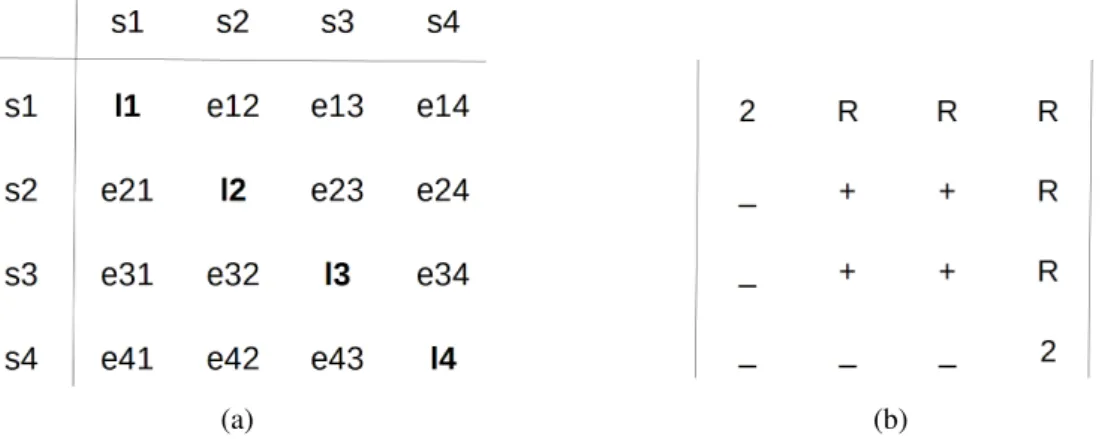
A SLG is a directed graph that can be visualized as an adjacency matrix of labels (Figure 2.7). Figure 2.7a provides the format of the adjacency matrix: the diagonal refers stroke (node) labels and other cells interpret stroke pair (edge) labels [Zanibbi et al., 2013]. Figure 2.7b presents the adjacency matrix of labels corresponding to the SLG in Figure 2.5c. The underscore ’_’ identifies that this edge exists and the label of it is N oRelation, or this edge does not exist. The edge e14 with the label of R is an inherited relationship which is not reflected in SLG as we said before. Suppose we have ’n’ strokes in one expression, the number of cells in the adjacency matrix is n2. Among these cells, ’n’ cells represent the labels of strokes while the other ’n(n − 1)’ cells interpret the segmentation information and relationships.

In order to analyze recognition errors in detail, Zanibbi et al. defined for SLGs a set of metrics in [Zanibbi et al., 2013]. They are listed as follows:

• ∆C, the number of stroke labels that differ. • ∆S, the number of segmentation errors. • ∆R, the number of spatial relationship errors.

(a) (b)

Figure 2.7 – Adjacency Matrices for Stroke Label Graph. (a) The adjacency matrix format: li denotes the label of stroke si and eij is the label of the edge from stroke si to stroke sj. (b) The adjacency matrix of labels corresponding to the SLG in Figure 2.5c.

• ∆L = ∆S + ∆R, the number of edge labels that differ.

• ∆B = ∆C + ∆L = ∆C + ∆S + ∆R, the Hamming distance between the adjacency matrices. Suppose that the sample ’2 + 2’ was interpreted as ’2 − 12’ as shown in Figure 2.8, we now compare the two adjacency matrices (the ground truth in Figure 2.7b and the recognition result in Figure 2.8b):

(a) (b)

Figure 2.8 – ’2 + 2’ written with four strokes was recognized as ’2 − 12’. (a) The SLG of the recognition result; (b) the corresponding adjacency matrix. ’Sup’ denotes Superscript relationship.

• ∆C = 2, cells l2 and l3. The stroke s2 was wrongly recognized as 1 while s3 was incorrectly labeled as −.

• ∆S = 2, cells e23 and e32. The symbol ’+’ written with 2 strokes was recognized as two isolated symbols.

• ∆R = 1, cell e24. The Right relationship was recognized as Superscript. • ∆L = ∆S + ∆R = 2 + 1 = 3.

• ∆B = ∆C + ∆L = ∆C + ∆S + ∆R = 2 + 2 + 1 = 5.

Zanibbi et al. defined two additional metrics at the expression level:

• ∆Bn = ∆B_n2 , the percentage of correct labels in adjacency matrix where ’n’ is the number of strokes. ∆Bnis the Hamming distance normalized by the label graph size n2.

• ∆E, the error averaged over three types of errors: ∆C, ∆S, ∆L. As ∆S is part of ∆L, segmentation errors are emphasized more than other edge errors ∆R in this metric [Zanibbi et al., 2013].

∆E = ∆C n + q ∆S n(n−1)+ q ∆L n(n−1) 3 (2.1)

We still consider the sample shown in Figure 2.8b, thus: • ∆Bn= ∆B_n2 = 5 42 = 5 16 = 0.3125 • ∆E = ∆C n + q ∆S n(n−1)+ q ∆L n(n−1) 3 = 2 4 + q 2 4(4−1)+ q 3 4(4−1) 3 = 0.4694 (2.2) Given the representation form of SLG and the defined metrics, ’precision’ and ’recall’ rates at any level (stroke, symbol and expression) could be computed [Zanibbi et al., 2013], which are current indexes for accessing the performance of the systems in CROHME. ’recall’ and ’precision’ rates are commonly used to evaluate results in machine learning experiments [Powers, 2011]. In different research fields like infor-mation retrieval and classification tasks, different terminology are used to define ’recall’ and ’precision’. However, the basic theory behind remains the same. In the context of this work, we use the case of seg-mentation results to explain ’recall’ and ’precision’ rates. To well define them, several related terms are given first as shown in Tabel 2.1. ’segmented’ and ’not segmented’ refer to the prediction of classifier while

Table 2.1 – Illustration of the terminology related to recall and precision. relevant non relevant

segmented true positive (tp) false positive (fp) not segmented false negative (fn) true negative (tn) ’relevant’ and ’non relevant’ refer to the ground truth. ’recall’ is defined as

recall = tp

tp + f n (2.3)

and ’precision’ is defined as

precision = tp

tp + f p (2.4)

In Figure 2.8, ’2 + 2’ written with four strokes was recognized as ’2 − 12_{’. Obviously in this case, tp is equal}

to 2 since two ’2’ symbols were segmented and they exist in the ground truth. f p is equal to 2 also because ’-’ and ’1’ were segmented but they are not the ground truth. f n is equal to 1 as ’+’ was not segmented but it is the ground truth. Thus, ’recall’ is ₂₊₁2 and ’precision’ is ₂₊₂2 . A larger ’recall’ than ’precision’ means the symbols are over segmented in our context.

2.2

Mathematical expression recognition

In this section, we first review the entire history of this research subject, and then only focus on more recent solutions which are provided as a comparison to the new architectures proposed in this thesis.

2.2.1

Overall review

Research on the recognition of math notation began in the 1960’s [Anderson, 1967], and several research publications are available in the following thirty years [Chang, 1970, Martin, 1971, Anderson, 1977]. Since the 90’s, with the large developments of touch screen devices, this field has started to be active, gaining amounts of research achievement and considerable attention from the research community. A number of surveys [Blostein and Grbavec, 1997, Chan and Yeung, 2000, Tapia and Rojas, 2007, Zanibbi and Blostein, 2012, Mouchère et al., 2016] summarize the proposed techniques for math notation recognition.

As described already in Section 1.2, ME recognition involves three interdependent tasks [Zanibbi and Blostein, 2012]: (1) Symbol segmentation, which consists in grouping strokes that belong to the same symbol; (2) symbol recognition, the task of labeling the symbol to assign each of them a symbol class; (3) structural analysis, its goal is to identify spatial relations between symbols and with the help of a grammar to produce a mathematical interpretation. These three tasks can be solved sequentially or jointly.

Sequential solutions. In the early stages of the study, most of the proposed solutions [Chou, 1989, Koschinski et al., 1995, Winkler et al., 1995, Lehmberg et al., 1996, Matsakis, 1999, Zanibbi et al., 2002, Tapia and Rojas, 2003, Toyozumi et al., 2004, Tapia, 2005, Zhang et al., 2005, Yu et al., 2007] are se-quential ones which treat the recognition problem as a two-step pipeline process, first symbol segmentation and classification, and then structural analysis. The task of structural analysis is performed on the basis of the symbol segmentation and classification result. Considerable works are done dedicated to each step. For segmentation, the proposed methods include Minimum Spanning Tree (MST) based method [Matsakis, 1999], Bayesian framework [Yu et al., 2007], graph-based method [Lehmberg et al., 1996, Toyozumi et al., 2004] and so on. The symbol classifiers used consist of Nearest Neighbor, Hidden Markov Model, Multi-layer Perceptron, Support Vector Machine, Recurrent neural networks and so on. For spatial relationship classification, the proposed features include symbol bounding box [Anderson, 1967], relative size and po-sition [Aly et al., 2009], and so on. The main drawback of these sequential methods is that the errors from symbol segmentation and classification will be propagated to structural analysis. In other words, symbol recognition and structural analysis are assumed as independent tasks in the sequential solutions. However, this assumption conflicts with the real case in which these three tasks are highly interdependent by nature. For instance, human beings recognize symbols with the help of structure, and vice versa.

Integrated solutions. Considering the natural relationship between the three tasks, researchers mainly focus on integrated solutions recently, which performs the task of segmentation at the same time build the expression structure: a set of symbol hypotheses maybe generated and a structural analysis algorithm may select the best hypotheses while building the structure. The integrated solutions use contextual information (syntactic knowledge) to guide segmentation or recognition, preventing from producing invalid expressions like [a + b). These approaches take into account contextual information generally with grammar (string grammar [Yamamoto et al., 2006, Awal et al., 2014, Álvaro et al., 2014b, 2016, MacLean and Labahn, 2013] and graph grammar [Celik and Yanikoglu, 2011, Julca-Aguilar, 2016]) parsing techniques, producing expressions conforming to the rules of a manually defined grammar. String grammar parsing, along with graph grammar parsing, has a high time complexity in fact. In the next section we will analysis deeper these approaches. Instead of using grammar parsing technique, the new architectures proposed in this thesis include contextual information with bidirectional long short-term memory which can access the content from both the future and the past in an unlimited range.

End-to-end neural network based solutions. Inspired by recent advances in image caption generation, some end-to-end deep learning based systems were proposed for ME recognition [Deng et al., 2016, Zhang et al., 2017]. These systems were developed from the attention-based encoder-decoder model which is now widely used for machine translation. They decompile an image directly into presentational markup such as LA_{TEX. However, considering we are given trace information in the online case, despite the final L}A_TEX

string, it is necessary to decide a label for each stroke. This information is not available now in end-to-end systems.

2.2.2

The recent integrated solutions

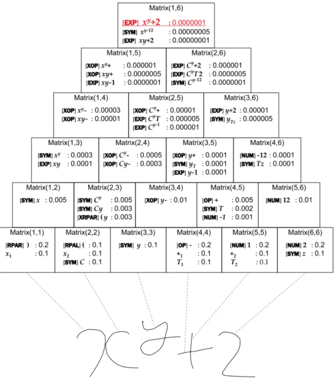
In [Yamamoto et al., 2006], a framework based on stroke-based stochastic context-free grammar is proposed for on-line handwritten mathematical expression recognition. They model handwritten mathe-matical expressions with a stochastic context-free grammar and formulate the recognition problem as a search problem of the most likely mathematical expression candidate, which can be solved using the Cock Younger Kasami (CYK) algorithm. With regard to the handwritten expression grammar, the authors define production rules for structural relation between symbols and also for a composition of two sets of strokes to form a symbol. Figure 2.9 illustrates the process of searching the most likely expression candidate with

Figure 2.9 – Example of a search for most likely expression candidate using the CYK algorithm. Extracted from [Yamamoto et al., 2006].

as following:

• For each input stroke i, corresponding to cell M atrix(i, i) shown in Figure 2.9, the probability of each stroke label candidate is computed. This calculation is the same as the likelihood calculation in isolated character recognition. In this example, the 2 best candidates for the first stroke of the presented example are ’)’ with the probability of 0.2 and the first stroke of x (denoted as x1 here)

with the probability of 0.1.

• In cell M atrix(i, i+1), the candidates for strokes i and i+1 are listed. As shown in cell M atrix(1, 2) of the same example, the candidate x with the likelihood of 0.005 is generated with the production rule < x → x1x2, SameSymbol >. The structure likelihood computed using the bounding boxes is

0.5 here. Then the product of stroke and structure likelihoods is 0.1 × 0.1 × 0.5 = 0.005.

• Similarly, in cell M atrix(i, i + k), the candidates for strokes from i to i + k are listed with the corresponding likelihoods.

• Finally, the most likely EXP candidate in cell M atrix(1, n) is the recognition result.

In this work, they assume that symbols are composed only of consecutive (in time) strokes. In fact, this assumption does not work with the cases when the delayed strokes take place.

In [Awal et al., 2014], the recognition system handles mathematical expression recognition as a simul-taneous optimization of expression segmentation, symbol recognition, and 2D structure recognition under the restriction of a mathematical expression grammar. The proposed approach is a global strategy allow-ing learnallow-ing mathematical symbols and spatial relations directly from complete expressions. The general architecture of the system in illustrated in Figure 2.10. First, a symbol hypothesis generator based on 2-D

Figure 2.10 – The system architecture proposed in [Awal et al., 2014]. Extracted from [Awal et al., 2014]. dynamic programming algorithm provides a number of segmentation hypotheses. It allows grouping strokes which are not consecutive in time. Then they consider a symbol classifier with a reject capacity in order to deal with the invalid hypotheses proposed by the previous hypothesis generator. The structural costs are computed with Gaussian models which are learned from a training data set. The spatial information used are baseline position (y) and x-height (h) of one symbol or sub-expression hypothesis. The language model is defined by a combination of two 1-D grammars (horizontal and vertical). The production rules are applied successively until reaching elementary symbols, and then a bottom-up parse (CYK) is applied to construct the relational tree of the expression. Finally, the decision maker selects the set of hypotheses that minimizes the global cost function.

A fuzzy Relational Context-Free Grammar (r-CFG) and an associated top-down parsing algorithm are proposed in [MacLean and Labahn, 2013]. Fuzzy r-CFGs explicitly model the recognition process as a fuzzy relation between concrete inputs and abstract expressions. The production rules defined in this grammar have the form of: A0

r

⇒ A1A2· · · Ak, where A0 belongs to non-terminals and A1, · · · , Akbelong

to terminals. r denotes a relation between the elements A1, · · · , Ak. They use five binary spatial relations:%

, →, &, ↓, . The arrows indicate a general writing direction, while  denotes containment (as in notations like√x, for instance). Figure 2.11 presents a simple example of this grammar. The parsing algorithm used

Figure 2.11 – A simple example of Fuzzy r-CFG. Extracted from [MacLean and Labahn, 2013]. in this work is a tabular variant of Unger’s method for CFG parsing [Unger, 1968]. This process is divided into two steps: forest construction, in which a shared parse forest is created from the start non-terminal to the leafs that represents all recognizable parses of the input, and tree extraction, in which individual parse trees are extracted from the forest in decreasing order of membership grade. Figure 2.12 show an handwritten expression and a shared parse forest of it representing some possible interpretations.

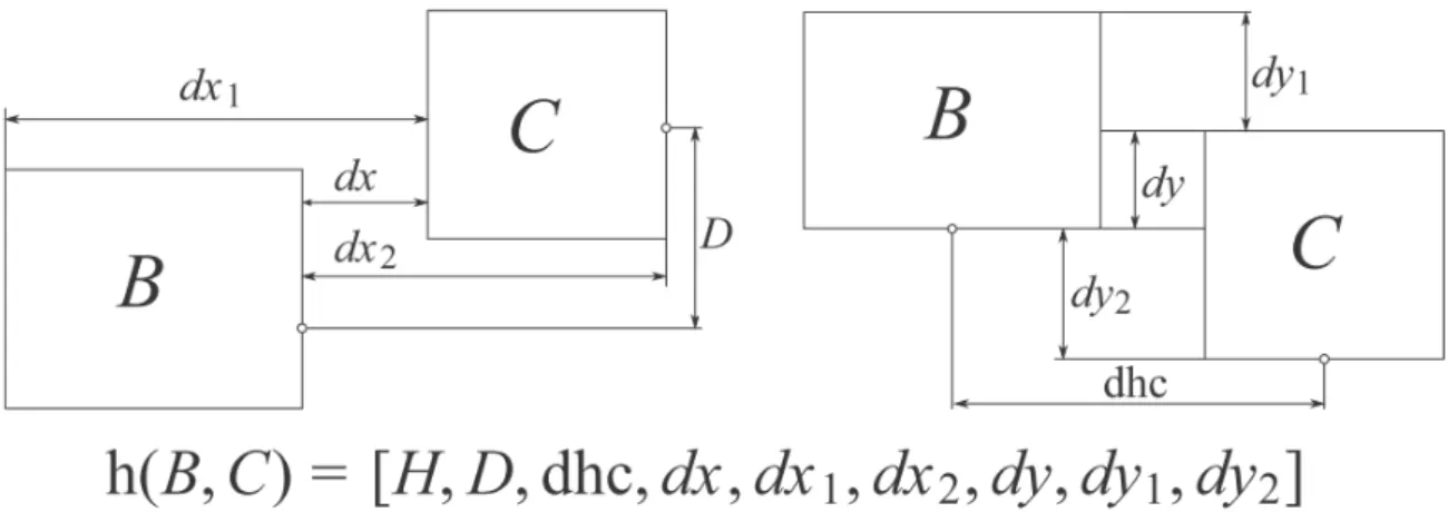
In [Álvaro et al., 2016], they define the statistical framework of a model based on Two-Dimensional Probabilistic Context-Free Grammars (2D-PCFGs) and its associated parsing algorithm. The authors also regard the problem of mathematical expression recognition as obtaining the most likely parse tree given a sequence of strokes. To achieve this goal, two probabilities are required, symbol likelihood and structural probability. Due to the fact that only strokes that are close together will form a mathematical symbol, a symbol likelihood model is proposed based on spatial and geometric information. Two concepts (visibility and closeness) describing the geometric and spatial relations between strokes are used in this work to characterize a set of possible segmentation hypotheses. Next, a BLSTM-RNN are used to calculate the probability that a certain segmentation hypothesis represents a math symbol. BLSTM possesses the ability to access context information over long periods of time from both past and future and is one of the state of the art models. With regard to the structural probability, both the probabilities of the rules of the grammar and a spatial relationship model which provides the probability p(r|BC) that two sub-problems B and C are arranged according to spatial relationship r are required. In order to train a statistical classifier, given two regions B and C, they define nine geometric features based on their bounding boxes (Figure 2.13). Then these nine features are rewrote as the feature vector h(B, C) representing a spatial relationship. Next, a GMM is trained with the labeled feature vector such that the probability of the spatial relationship model can be computed as the posterior probability provided by the GMM for class r. Finally, they define a CYK-based algorithm for 2D-PCFGs in the statistical framework.

Unlike the former described solutions which are based on string grammar, in [Julca-Aguilar, 2016], the authors model the recognition problem as a graph parsing problem. A graph grammar model for mathe-matical expressions and a graph parsing technique that integrates symbol and structure level information are proposed in this work. The recognition process is illustrated in Figure 2.14. Two main components are involved in this process: (1) hypotheses graph generator and (2) graph parser. The hypotheses graph generator builds a graph that defines the search space of the parsing algorithm and the graph parser does the parsing itself. In the hypotheses graph, vertices represent symbol hypotheses and edges represent relations

(a)

(b)

Figure 2.12 – (a) An input handwritten expression; (b) a shared parse forest of (a) considering the grammar depicted in Figure 2.11. Extracted from [MacLean and Labahn, 2013]