Application of Active Contour Models in Medical Image Segmentation

Application of Active Contour Models

in Medical Image Segmentation

M. KHELIF, F. DERRAZ , M. BELADGHAM FACULTE DES SCIENCES DE L'INGENIEUR;

UNIVERSITÉ A BELKAID -TLEMCEN B.P 230, TLEMCEN (13 000), ALGERIE

Abstract: Recent developments on medical imaging techniques have brought a completely new research field on image processing. The principal aim is to improve medical diagnosis through segmented images. Techniques have been developed to help for identifying specific structures within a magnetic resonance image: MRI. The Active Contour methods, these methods are adaptable to the desired features in the image . In our work, we describe two classes of active contour models and discussing application aspects in medical imaging area.

Keywords: MRI, Segmentation, active contour, parametric model, geometric model.

I.INTRODUCTION:

T

echniques of image processing are more and more used in medical field. Mathematical algorithms of feature extraction, modelling and measurement can be exploited in the images to detect pathology, evolution of the disease, or to compare a normal subject to abnormal one.

The advance of medical imaging devices has realised several developments in modern medicine and most of them in magnetic resonance imaging:MRI. These techniques provide detailed, non-invasive diagnosis of most human body structures. A second development have provided by coupling some computational techniques to help specialists to analyze the enormous amount of data contained in medical images. The aim of these methods is extracting and analyzing scientifically relevant and clinically important pieces of information from the original set of images.

One of the most important applications is, hence, the segmentation of specific structures. These methods make possible the application of mathematical or geometrical models on the steps of description and analysis of the acquired information.

Image segmentation is a fundamental issue in biomedical imaging area. Segmenting structures from medical images and the reconstruction of a compact analytic representation of these structures is difficult. This difficulty was due to the sheer size of the data sets and the complexity and variability of the anatomic shapes of interest.

The active contour method is one of the most successful image segmentation techniques, it has received a tremendous amount of attention in medical image processing. The segmentation operation can carried out manually or automatically. A manual segmentation requires a skilled operator trained to use a digital tool to mark the contours of the desired structures.

An obvious disadvantage is that an exhaustive process, where the results are hardly repeatable. Automatic techniques

usually apply evolving interfaces dynamically adaptable to the desired features contained in the image. The difference between the two techniques is whether or not the user is involved the process.

In this work, we are mainly concerned about the application active contour model in medical image segmentation. The paper is organised as follows. In next section we gives an overview theoretical background of the existent active contour model and we describe the two classes of active contour models, specially the Snakes model proposed by Kass et al [1] and the Level Set Method presented by Sethian [2]. The main features, advantages and disadvantages of the models are discussed.

Section III contains an application of the two classes of active contour in medical image area, illustrated by some experiment results.

II.BACKGROUND ON ACTIVE CONTOUR MODELS:

Active Contour models define interfaces on the image domain, which can move accordingly to internal forces and external forces derived from image characteristics. The external forces are defined as the gray-level gradient. There are two types of active contour models: the parametric models, such as the Snakes [1], and the geometric models, like the Level Set method [2-13]. The first models define an elastic contour which can dynamically adapt to desired edges of objects in the image. This adaptation occurs in response to both forces. An algorithm that implements this model must keep contour representation during the calculation. The second ones use a different approach, as they embed the front as the zero level set of a higher dimensional function, and then calculate the evolution of this new function. This evolution is dependent on characteristics extracted from the image and geometric restrictions of the function itself.

II.1PARAMETRIC MODELS:

The original parametric active contour model was introduced by Kass, Witkin and Terzopoulois [1], and is known as Snakes, due to the way the contour moves to its final position. In this model, the contour has a initial user, specified position and an associated objective function defined as the energy of the snake. The snake may then be defined as a curve v

( )

s =

[

x

( ) ( )

s,

( )

ys

]

, s∈

[ ]

0,1 which moves in the image domain to minimize the energy function [5] shown below:

( )

( )

( )

( )

∫

      +       ₊ = 1 0 2 '' 2 ' 2 1 _{v s v s E vs ds} E α β _ext (1)

The first part of the integral is related to the snake’s internal energy, and imposes restrictions to its movement by controlling the elasticity and stiffness parameters, which are weighed by α and β, respectively. The second part stands for the external energy, and is responsible for driving the snake towards important features in the image, e.g. edges of specific body structures in a MR image.

For a given gray-level image I ,

( )

x y , this internal energy

int E is identified as:

( )

( )

∫

_ _ + __ = 1 0 2 '' 2 ' int ₂1 v s v s ds E α β (2.a)

and the external energy can be written as:

( ) ( )

(

)

2 , ,y I x y x G E_ext =−∇ _σ ∗ (2.b)

where G_σ is a two dimensional gaussian filter with a standard deviation σ and ∇ is the gradient operator. This filter is applied to the image in order to improve the image’s edge map, and also to perform some noise reduction [4]. So, on regions closer to edges the gradient term yields high values. A local minimum to (1) can be found by resolving the Euler-Lagrange equation on v ( )

_{( )}

( )

_{( )}

ext E s v s v2 −_β 4 =∇ α (3)

This equation represents a force balance condition, where the term αv( )2

( )

s −βv( )4

( )

s corresponds to the internal forces and ∇E_ext =0 to the external, image-derived forces. By treating v

( )

s as a time-dependent function, and supposing that a solution is available wheret =0. The snake’s evolving equation is expressed as:

( )

_{, =} ( )2

_{( )}

_{, −} ( )4

_{( )}

_{, −∇ =0}

ext t st v s t v st E

v α β (4)

When the snake reaches steady state, a solution is found to (3). The model is solved numerically by using finite difference techniques, as shown by Kapur et al in [6].

In this works, we consider a discrete active contour model defined using finite difference approximations of the derivative in (4).

Despite the model’s consistency and simplicity, there are some performance problems associated to it [2]. For example, the initial position of the snake must be close to the desired contour in the image, otherwise the snake may not evolve correctly, as it may find local minima away from the contour. Another common problem is that equation (4) can produce meaningless results. This problem can happen every time

there are concavities or sharp corners in the gray-level image. Further more, the snake is indivisible, that is, it cannot split itself into two or more separated entities to adapt themselves to topological changes in the image domain. Fortunately, there is a number of solutions to the above problems, although each of them usually brings additional complexity to the model, and sometimes, new problems.

Most solutions define additional terms added to the external force component of equation (3), as a way to improve the snake’s capture range and force it towards the image edges. The initialization problem can be improved by adding a constant normal force component to the external force term.

( )

ext ext ext _E E k s n k F = ~₁ − ∇ (5)

This is the Balloon model proposed by Cohen in [7]. The snake may then inflate or deflate, depending on the sign and magnitude (k1) of the balloon force. Although the balloon

model prevents the snake from stalling in homogeneous regions of the image (hence in-creasing its capture range), special care must be taken to choose appropriate values to k and k₁ in order to make the balloon force strong enough to make the snake overcome weak edges and noise, but without overshooting a desired contour. In [7,22] Cohen has proposed a different external force model as gradient potential function computed using Euclidean distance map. These forces are referred to as distance potential forces, because they have higher values farther away from the edges of interest. This model also improves the initialization problem, but does nothing to make the snake more adaptable to sharp corners and concave regions. The latter problems could only be diminished by another external force model proposed by Xu and Prince in [4,5,23]. Their model, the Gradient Vector Flow : GVF, produces a field with strong forces near the edges, but also extending the gradient map farther into homogeneous regions using a computational diffusion process, which is also responsible for creating vectors that point into boundary concavities. The gradient vector flow was then defined as the vector field g

( )

x,y =

(

u

( ) ( )

x,y,vx,y

)

that minimizes the energy function:

(

ux uy vx vy

)

f g f dxdy 2 2 2 2 2 2

∫∫

+ + + +∇ −∇ = µ ε (6)

where f

( )

x,y = ∇G_σ

( ) ( )

x,y ∗I x,y is defined as the edge map function for a gray-level image.

The field ∇f has vectors pointing toward the edges, but it has a narrow capture range, in general. Furthermore, in homogeneous regions, I

( )

x,y is constant, ∇f is zero, and therefore no information about nearby or distant edges is available.

From (6) we see that when ∇f is small, the energy is dominated by the partial derivatives of the vector field, yielding a smooth force field. In other terms, for larger values of ∇f , the second term dominates the integrand and is minimized wheng=∇f . This ensures that

g

will be just

like the edge map gradient when it is large, but also forces the vector field to vary smoothly in homogeneous regions. The parameter µ establishes the trade-off between the first and second terms, and should be set directly according to the amount of noise in the image. We note that the first smoothing term within the integrand of (6) leads to the Laplacian operator in the corresponding Euler equations. It has recently been shown that this term corresponds to an equal penalty on the divergence and curl of the vector field [8]. Therefore, the external field resulting from this minimization can be expected to be neither entirely ir rotational norontirely solenoidal. We refer the reader more detailed solution to [4,5,23].

Another model, denominated Dual Active Contour [8,14,15], uses a pair of snakes approaching the desired contour from both inner and outer sides, as a way to improve the detection of global minima. This improves the initial position limitations, as well as the evaluation of the stiffness and elasticity parameters. As disadvantages, we may cite its complex implementation and low computational efficiency. All models shown above, although solving some of the problems faced by the original Kass et al. model [1], still aren’t able to deal with topological changes on the snake contour. This technique solves the initialization problem and provides a more robust snake evolution, despite of its complex implementation. Some experiments are given’s in last section using the GVF model [4,5] to extract specific shapes from a selected MR image.

II.2 Geometric models

The geometric models where first proposed by Sethian in [10]. It defines a front evolving according to a given curvature dependent speed functionF. This function can also depend on the image gradient [4,23]. When the speed function is monotonic. We can defines a geometric models based on the Level Set evolution curve.

II.2.1 The level set approach

The main idea of this model is to, instead of actually parameterizing the front S

( )

t , represent it as the zero level set of a higher dimensional function φ , and calculate the evolution of this function as a initial value problem. This can be modeled as: 0 = ∇ + ∂ ∂φ _φ F t (7)

given φ

(

s,t =0

)

. At any instant, the position of front S

( )

t

shall be given as the zero level set of the evolving function φ

( ) ( )

_{t =}

{

_x,_{y ∈R}2

(

_x,_y,_t

)

₌0

}

S φ (8)

The speed scalar functionFdepending on:

- Local proprieties of the front, like the local curvature.

- External parameters related to the image gradient. - additional propagation terms.

This should work in a similar way to the external snake energy shown previously, leading the evolving front towards the desired contours in the image. A common choice for Fis [2,10]:

(

k

) ( )

g x y F= ±1+ε _I , (9)

where ε is a constant

(

0<ε<1

)

, k is the local curvature of the level set functionφ . This curvature can be defined as:

(

)

2 3 2 2 2 2 ₂ . y x x yy xy y x y xx k φ φ φ φ φ φ φ φ φ φ φ + + − − = ∇ ∇ ∇ = (10)

The term g_I

( )

x,y is an image-dependent halting criteria calculated as:

( )

₍

_{( )}

₎

y x I G y x gI , ₁ 1_{* ,} σ ∇ + = (11)

which works in a similar manner than the snake’s external energy defined in equation (2), as it yields smaller values when closer to higher gradients in the image, bringing equation (9) to very low values and consequently slowing down the evolution of the front

S

. The uniform expansion or contraction with speed respectively 1 or -1 corresponds to pressure forces defined in the balloon snake model [7]. Other more complex speed function definitions are discussed in [2,11].

The diffusive term εκ has a smoothing effect and also acts as a restriction term just like the internal energy term of the original snake model.

A numerical solution for equation (7) can be developed from an explicit finite difference approximation of the time gradient 0 1 = ∇ + ∆ − + n ij ij n ij n ij _F t φ φ φ (12)

where the unknown value of the function in the new time step

1 +

n ij

φ is calculated from the values derived in the previous time step φ_ijn . This formulation is then made more stable than the parametric models by using a different set of approximations to the gradient of φ . According to Sethian [10], a central difference scheme, for example, would fail in points where the front develops a sharp corner, and the singularity introduced would propagate numerical errors throughout the iteration process. For that matter, a better set of approximations can be obtained by using hyperbolic schemes over Hamilton-Jacobi equations [10,2], which would converge to the right viscosity solution while keeping a smooth and homogeneous front. Equation (12) would then be approximated as:

( )

( )

[

+ −

]

+ ∇ + ∇ = ∆ − 0 , min 0 , max 1 ij ij n ij n ij _{F F} t φ φ (13)

(

)

(

)

(

)

(

)

2 1 2 2 2 2 0 , min 0 , max 0 , min 0 , max           + + + = ∇ + − + − + φ φ φ φ y ij y ij x ij x ij D D D D (14)

(

)

(

)

(

)

(

)

2 1 2 2 2 2 0 , min 0 , max 0 , min 0 , max           + + + = ∇ − + − + − φ φ φ φ y ij y ij x ij x ij D D D D (15)

and the differential operators D−andD+ stand for left and right finite difference approximations, respectively, as shown below : x D n j i n j i x ij _∆ − = − − _φ φ, φ 1, x D n j i n j i x ij _∆ − = + + _φ φ 1, φ, (16) y D n j i n j i y ij _∆ − = − − _φ φ, φ, 1 y D n j i n j i y ij _∆ − = + + _φ φ, 1 φ, ₍₁₇₎

A numerical algorithm to solve the previous sets of equations should iteratively solve (13) for each point in the domain, until a steady situation is found. As this equation is explicit in time, a stability criteria must be defined to correctly choose the time step ∆t. As shown by Sethian [2], the front should not cross more than one grid point per time step, such that

x t F∆ )≤∆

max( (18)

where the maximum value has to be searched over the entire image domain. If we had a square uniform grid, with n nodes in both directions x and y, and supposing that k iterations would be needed to reach the steady state, its computational complexity would be O(kn2). Alternatively, Adalsteinsson and Sethian [12] propose to focus the calculations over a narrow band immediately close to the front. Equation (13) could then be applied to a much smaller set of points, sensitively decreasing the computational complexity toO(bkn), where b would be the width of the narrow band. As the front approaches the edges of the narrow band, the calculation would be halted and a new narrow band would be defined.

This formulation should be used whenever the front S

( )

t is allowed to move in any direction. A very common and much simpler situation occurs when the front moves in only one direction, defined by a monotonic speed function F.

First of all, the initialization details have to be commented. The level set functionφ must satisfy the property ∇φ =1, preserving its configuration as a signed distance function of the front S

( )

t , for all time [2]. So, if the initial configuration of

S

is a single point,φ is constructed to ensure that all its level sets are equidistant to the zero level set

S

. Supposing a constant uniform speed function F =1 acting on the above defined level set function φ , we might expect that the initial point would expand indefinitely as a larger circle each iteration. This is the basic idea of the Level Set Method. The next step is to use a gray level gradient-driven speed function, as defined in equation (9) to evolve φ towards the desired contours. Unfortunately, although F is now a real, non-uniform function, defined only over F. The algorithm doesn’t see it that way, considering F valid over the entire domain. It then updates all level sets of φ according toF, causing φ to be no longer a signed distance function where

1 =

∇φ .

This complication is briefly discussed in [2,10-13] by Sethian and additional framework is provided. One of the solutions presented is to periodically stop the calculations and reconstruct the signed distance function φ according to the current position of S

( )

t . This is a complex and expensive

procedure, as it should be repeated every iteration to avoid errors. A second solution proposes to evaluate a extended velocity function F_ext, which is valid over the entire domain plus coinciding with F over φ . Since F_ext should also correspond to a signed distance function, it would have to satisfy 0 = ∇φ ext F (19)

Although this alternative is said to bring more accurate results, its implementation is far from simple. Furthermore, the construction of an extension velocity function contradicts the most appealing feature of the method since it requires to actually build a explicit representation of the front S

( )

t . A similar way to do this without actually building a explicit representation of

S

is discussed by Gomes and Faugeras [13]. There is still the possibility of periodically reinitialize

φ as a signed distance function that satisfies ∇φ =1. This would require to solve:

( )

φ

(

φ

)

φ _{= −∇} ∂ ∂ 1 sign t (20)

to reorganize the level sets on both sides of

S

. Although this is a simpler alternative, it doesn’t consider the actual position of the front, leading to positioning errors.

III Experiment results:

In this section we show how the previous active contour models, both parametric and geometric, can be applied to medical image segmentation.

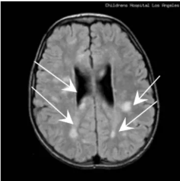
In order to show the interests of the segmentation by active contour models. We select an MR image of 256x256 pixels. This image is selected from image database set[24]. The image represents slice brain attained of tumours pathology.

Fig 1. Transaxial slice brain image corresponding to child of the 8 year old with tumours depicted.

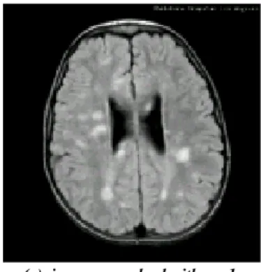
In order to segment the pathology in brain slice image, we must proceed initially by an operation of pre-treatment, this consists of application of the Gaussian filter to the initial image. A comment choice of σ is fixed between 0.1 and 1.

(a) image convolved with σ =1.

Fig 2. Pathological image convolved with a Gaussian filter Gσ As shown in figure (2), the edge map shows higher values where the image gradient is larger, and low values over homogeneous regions. Fig 2 shows how the Gaussian filter blurs the edges, thus increasing the snake’s capture range as it spreads the force vectors along the potential field.

Using a traditional snake model and a fair initial position, we can see that it correctly evolves towards the desired contour, in figure 3, we show for adequate choice of snakes parameter α and β.

For several experiments, we have fixed set of pairs (α,β). The experiments where done for α=1, and β=0.03 . This pair of (α,β) has drown agree results. And isolate correctly the tumours.

(a ) initial contour (b) final contour Fig3. Pathological image segmented with classical parametric active contour models

On the other terms, if some parts of the snake (or all of it) where initialized over homogeneous regions of the image, the contour wouldn’t evolve correctly, stalling where the force field vectors have lower magnitude (fig 3).

In adding the balloon model, it makes the snake less dependent on its initialization, by the use of pressure forces. The GVF model also improves the problems related to bad initial position without using pressure forces. Be-sides, this model doesn’t need a previous knowledge about whether the snake will grow or shrink, as does the Balloon model. However, it’s important not to overestimate the GVF snake initialization capability. If it is done way too distant of the desired contour, the snake may take a very long time to converge or even stall over homogeneous regions. The GVF model has shown better performance and more accurate results than the traditional, Balloon or Distance Vector models.

But, it's also hard for fixing a good of parameter, that leeds to locate the tumours area in the brain slice. After several test,

for selecting the adequate parameters, it achieved for experiments values: α=1, β=0.03 , µ=1.2 and g=0.8

(a ) initial contour (b) final contour Fig 4. Segmentation of a tumour in an MRI brain data

by the parametric active contour model (GVF)

(a ) initial contour (b) final contour Fig 5. Segmentation of a tumour in an MRI brain data by the geometric active contour model (Level Set Method )

In the second experiment, the pathology is segmented by fixing of the speed function equal to several values between F= 1 and F=2 . We observe that for F=1, the tumours area segmented is more less then in the case of the parametric contour. The contour follows to best the edges of the pathologies.

The area of tumours is more less then that detected for parametric active contour models.

To compare the results drawn both by the parametric and geometric model. The key difficulty when working with active contour models is the correct definition of both the external energy term and speed function. Since both are based on the image gradient, one might expect similar behavior to both models. Problems related to bad initialization, local minima, and incorrect convergence may happen when working with either model, unless proper care is taken. Parametric model was be a more simple way than the geometric, regarding both the contour representation and implementation complexity. The explicit formulation of a evolving closed contour searching for a energy function minimization is far more intuitive. One may question about the Snake’s lack of robustness when dealing with sharp corners, topological changes and initialization problems, but as we have shown, there is no ideal method, only specific procedures to ensure the correct result obtained from specific image sets. On the other terms, the mathematical formulation of geometric models is more robust. Issues like topological changes and sharp corners are dealt with naturally. What is left to complain about is the lack of information regarding the

actual algorithm implementation of both the Level Set Method due to problems when defining the correct extension velocity function

IV Conclusions

The main conclusion from this work is that there is no ideal segmentation method. Both parametric and geometric active contours are driven by forces extracted from the image itself, what makes them extremely dependent on the image quality, that is, lowly noised, fair definition of the structures’ edges and absence of local minima. Even if one is able to overcome these problems, there are still further difficulties, like the initialization problem for example, which has a strong impact on the correct contour’s convergence. This kind of problem may cause the procedure to be repeated until the result obtained is good enough for the user.

Finally, it is important to observe that an efficient, precise medical image segmentation system should necessarily add to the model some level of intrinsic knowledge about the problem. Variables like the kind, shape and relative location of the common structures or pathology, and their size compared to some reference system such as a anatomy atlas[20], would improve enormously the model’s robustness and autonomy.

References

[1] M. Kass, A. Witkin and D. Terzopoulos, “Snakes: Active Contour Models,” International Journal of Computer Vision, 1(4): 321-331, 1988.

[2] J. A. Sethian, “Level Set Methods and Fast Marching Methods,” Evolving Interfaces in Computational Geometry, Fluid Mechanics, Computer Vision and Materials Science., 1st. ed.. Cambridge University Press, 1999.

[3] J. A. Sethian, “Tracking Interfaces with Level Sets,” American Scientist, May-June, 1997.

[4] C. Xu and J. L. Prince, “Gradient Vector Flow: A New External Force for Snakes,” IEEE Proceedings on Computer Vision and Pattern Recognition, 66-71, 1997.

[5] C. Xu, J. L. Prince. Snakes, “Shapes and Gradient Vector Flow,” IEEE Transactions on Image Processing, 359-369, 1998.

[6] T. Kapur, W. E. L. Grimson and R. Kikinis, “Segmentation of Brain Tissue MR Images,” First Conference on Computer Vision, Virtual Reality and Robotics in Medicine, 1995.

[7] L. D. Cohen, I. Cohen, “Finite Element Methods for Active Contour Models and Balloons for 2D and 3D images,” IEEE Transactions on Pattern Analysis and Machine Intelligence, 1993.

[8] S. R. Gunn, M. S. Nixon, “A Robust Snake Implementation: A Dual Active Contour,” IEEE Transactions on Pattern Analysis and Machine Intelligence, 19, 63-68, 1997.

[9] T. McInerkey, D. Terzopoulos, “Topologically Adaptable Snakes,” Proceedings of the Fifith International Conference on Computer Vision, 840-845, 1995.

[10] J. A. Sethian, “Numerical Methods for Propagating Fronts,” Variational Methods for Free Surface Interfaces, Proceedins of the Vallambrosa Conference, 1987.

[11] R. Malladi, J. A. Sethian, ”A O(N log N) Algorithm for Shape Modelling,”. Proceedings of the National Academy of Sciences, Vol. 93, 9389-9392, 1996.

[12] D. Adalsteinsson, J. A. Sethian.“A Fast Level Set Method for Propagating Interfaces,” Journal of Computational Physics, Vol. 118, 269-277, 1995.

[13] J. Gomes, O. Faugeras, “Reconciling Distance Functions and Level Sets,” Proceedings of the Second International Conference on Scale-Space Theories in Computer, 1999. [14] G. A. Giraldi, E. Strauss and A. A. F. Oliveira, “A Boundary Extraction Approach Based on Multi-Resolution Methods and the T-Snakes Framework”. DEL, UFRJ, 2000. [15] T. McInerkey, D. Terzopoulos, “A Dynamic Finite Element Surface Model for Segmentation and Tracking Multidimensional Medical Images with Application to Cardiac 4D Image Analysis,” Journal of Computerized Medical Imaging and Graphics, 1994.

[16] T. McInerkey, D. Terzopoulos, “Medical Image Segmentation Using Topologically Adaptable Surfaces,” Third Conference on Computer Vision, Virtual Reality and Robotics in Medicine, 1997.

[17] R. Malladi, J. A. Sethian. “A Unified Approach to Noise Removal, Image Enhancement and Shape Recovery,” IEEE Transactions on Image Processing, 5, 11, 1154-1168, 1996. [18] J. A. Sethian. “A Fast Marching Level Set Method for Monotolically Advancing Fronts,” Proceedings of the National Academy of Sciences, 93, 4, 1591-1595, 1995. [19] J. A. Sethian. “Fast Marching Methods and Level Set Methods for Propagating Interfaces”. von Karman Institute Lecture Series, Computational Fluid Mechanics,1998. [20] M. Sonka, J. M. Fitzpatrick.”Handbook of Medical Imaging Vol. 2: Medical Image Processing and Analysis,” SPIE Optical Engineering Press, 2000.

[21] D. Williams and M. Shah. “A Fast Algorithm for Active Contours and Curvature Estimation,” CVGIP: Image Understanding, 55, 1, 14-26, 1992.

[22] L.D. Cohen, “On active contour models and balloons,” CVGIP: Image Understanding, vol.53, pp. 211-218, 1991. [23] C. Xu and J.L. Prince, “Generalized gradient vector flow external forces for active contours,” Signal Processing, vol. 71, pp. 131-139, 1998.