HAL Id: hal-00978682
https://hal.archives-ouvertes.fr/hal-00978682
Submitted on 16 May 2020HAL is a multi-disciplinary open access
archive for the deposit and dissemination of sci-entific research documents, whether they are pub-lished or not. The documents may come from teaching and research institutions in France or abroad, or from public or private research centers.
L’archive ouverte pluridisciplinaire HAL, est destinée au dépôt et à la diffusion de documents scientifiques de niveau recherche, publiés ou non, émanant des établissements d’enseignement et de recherche français ou étrangers, des laboratoires publics ou privés.
Borghi, Pierre Philippe
To cite this version:
Fabienne Mercier, Frederic Golay, Stéphane Bonelli, Fabien Anselmet, Roland Borghi, et al.. 2D axisymmetrical numerical modelling of the erosion of a cohesive soil by a submerged tur-bulent impinging jet. European Journal of Mechanics - B/Fluids, Elsevier, 2014, 45, pp.36-50. �10.1016/j.euromechflu.2013.12.001�. �hal-00978682�
Postprint accepted - The European Journal of Mechanics - B/Fluids
2D Axisymmetrical Numerical modelling of the
erosion of a cohesive soil by a submerged
turbulent impinging jet
Mercier F.(1),(5), Golay F.(2), Bonelli S.(1), Anselmet F.(3), Borghi R.(4), Philippe P.(1)
(1)Irstea, 3275 Rte Cézanne, CS 40061, 13182 Aix-en-Provence Cedex 5, France (2)Université de Toulon, Imath, EA 2134, 83957 La Garde, France
(3)IRPHE, Technopôle de Château-Gombert, 49 rue Joliot Curie, BP 146, 13384 Marseille
Cedex 13, France
(4)ECM, Technopôle de Château-Gombert, 38 rue Frédéric Joliot-Curie, 13451 Marseille
Cedex 20
(5)GeophyConsult, Savoie Technolac, 12 allée du lac de Garde, BP 231, 73374 Le Bourget du
Lac Cedex, France
Corresponding Author: Fabienne Mercier – [email protected]
Fabienne Mercier
Irstea, 3275 Rte Cézanne, CS 40061 13182 Aix en Provence Cedex 5 France
Abstract: This study focuses on 2D Computational Fluid Dynamics (CFD) numerical modelling of the erosion of a cohesive soil by a circular impinging turbulent jet. Initially, the model is validated in the case of a non-erodible flat plate. Several turbulence models are compared to experimental results and to simplified formulas available in the literature. The results obtained show that the Reynolds Stress Model (RSM) is in good agreement with the semi-empirical results in the literature. Nonetheless, the RSM cannot be used with successive remeshings, due to its convergence issues. The shear stress at the wall is well-described by the
k-
ε
model while the pressure is better-described by the k-ω
model. The numerical model of erosion is based on adaptive remeshing of the water/soil interface to ensure the good precision of the mechanical values at the wall. The two erosion parameters are the critical shear stress and the erosion coefficient. The results obtained are compared with the semi-empirical model interpreting the Jet Erosion Test. The k-ε
model underestimates the shear stress and does not allow simulating the entire erosion process, whereas the results obtained with the k-ω
model agree well with the semi-empirical model and experimental data. A study of the influence of erosion parameters on erosion kinetics and scouring depth shows that the shape and depth of scouring are influenced solely by the critical shear stress while the duration of scouring depends on both erosion parameters. Further research is nonetheless required to better understand the erosion mechanisms in the stagnation zone.Key-words: Erosion; Jet Erosion Test; critical shear stress; erosion coefficient; turbulent flow modelling; fluid-structure interaction modelling
1. Introduction
Soil erosion caused by a flow of water is an old but still topical issue. It deals with the fields of sediment transport and free surface flows. The phenomenon is considered globally, as a balance between detachment, transport and deposit of solid particles within a stationary flow. At a smaller scale, though one which remains that of a continuous medium, one of the first mechanically-based numerical simulation approaches was proposed by Vardoulakis et al. [1] in the field of petroleum geomechanics. It introduced a fluidised solid phase that presented a regular transition between the solid and liquid phases. These three phases were in interaction through a source term in the mass conservation equation. This source term describes the exchanges of mass between the three phases. It represents the erosion of the solid phase. Ouriemi et al. [2] have recently proposed a diphasic model in which the solid and liquid phases are in interaction through a source term in the equation of momentum conservation. This source term describes the exchanges of momentum between the two phases. It permits describing the erosion of the solid phase. These two approaches are well-adapted to a flow of water on a granular soil with sufficiently high permeability to allow the development of a fluidised solid phase between the flow and the granular medium. The flow of water is described by the Navier-Stokes equations, the intermediate zone by a Brinkman model and the flow in the granular medium by a Darcy model.
When the eroded soil is fine with a very low permeability, the thickness of this intermediate zone is very small. It is therefore more pertinent to consider that the interface between the flow and the soil is a singular interface, susceptible of being one of discontinuity. Erosion can therefore be described by the flux of eroded mass crossing this interface. This approach was proposed in particular by Brivois et al. [3] in the framework of a diphasic erosion model, then validated by Lachouette et al. [4].
A diphasic model of the flow is not necessary when erosion kinetics is very low in relation to flow velocity. Indeed, the flux of eroded mass is sufficiently low and the water flow sufficiently fast to allow assuming that the fluid phase is a diluted suspension, and that the exchanges of momentum between the water and the dispersed solid phase are negligible. In the case of a laminar flow, this hypothesis of low erosion kinetics has led to a monophasic model of erosion by an incompressible Stokes flow [5]. The numerical model unifies the description of the fluid and soil using the fictitious domains approach, on a fixed and independent Cartesian mesh. The fluid/soil interface is described by the level-set method Osher et al. [6].
For a turbulent flow, the model with a sharp interface was initially developed analytically, in the specific case of piping flow with erosion [7]. The case of a turbulent flow eroding a soil with slow erosion kinetics has still not been approached in a general way, thus this is what we propose to do in the present article, using a specific configuration: an impinging jet on a soil. Erosion modelling requires precise modelling of wall quantities, something that is particularly difficult in the case of turbulent flows. The fictitious domains method is therefore not relevant and another method has to be used.
To our knowledge, no work has yet been published on modelling the erosion process of a soil subjected to the impingement of a submerged jet flow. The geometry of a jet with a stagnation point on a flat surface is simple but its physics is complex. For high Reynolds numbers, the use of Reynolds Average Navier Stokes (RANS) models is common. The turbulence models most frequently used for modelling jet flows belong to the following three main categories of turbulence models, described in section 2: the model [8], the model [9] and the RSM (Reynolds Stress Model) model [10]. Looney et al. [11] presented results given by
several versions of the model. Craft et al. [12] compared a model with three RSM models. Jaramillo et al. [13] focused on using a turbulence model. Balabel and El-Askary [14] compared the performances of several and v²-f [15] turbulence models. Generally, these studies compared the influence of different turbulence models on calculation results for mean and fluctuation values of velocity, as well as for variables related to heat transfer, such as the Nusselt number and the heat transfer coefficient. To our knowledge, no numerical study on the subject of impinging jets has focused on pressure fields or the stress distribution on the impinged surface.
Direct numerical simulations (DNS) and large eddy simulations (LES) can lead to better understanding of fluid-soil interaction mechanisms and therefore the processes involved in erosion, but implementing these methods is still very difficult and costly in terms of the calculation time required to model erosion processes. The use of hybrid RANS/LES method could have been a good compromise but still remains time costly.
The present work focuses on the numerical modelling of a turbulent jet flow impinging a fine cohesive soil, causing its erosion. We will compare the results of the numerical model with the semi-empirical approach of the Jet Erosion Test introduced by Hanson and Cook [16]. In this paper, emphasis will be mainly given to the development and validation of the numerical modelling.
The paper is organised as follows: we will describe the physical model in section two and the numerical model in section three. The method for modelling the submerged impinging jet flow will be described in section four, with validation on a non erodible flat wall. In section five, we will present the results of the numerical modelling with erosion. The results will then be discussed in section six.
2. Flow model with erosion
2.1. Field equations
We study the surface erosion of a soil subjected to a turbulent flow. The soil particles are detached and then transported by the flow. The fluid domain is denoted Ω . The fluid flow w
equations are the following: 0 ( ) u u u u T w t
ρ
∇⋅ = ∂ + ∇ ⋅ = ∇⋅ ∂ in Ω w (1)where u is the mean velocity of the flow,
ρ
w the fluid specific density and T the Cauchy stress tensor. This stress tensor is expressed as follows:2 T= − +pI
µ
wD R+ in Ω w (2) , (3)where is the mean static pressure,
µ
w the molecular viscosity of the water, thesymmetrical part of the mean velocity gradient and the turbulent stress tensor (Reynolds stresses). This tensor is defined by the velocity fluctuations in comparison to the mean velocity . It has to be modelled by a turbulence model that will be described further in the paper.
2.2. Equations on the interface
The solid/fluid interface is denoted by . This interface, crossed by the flux of eroded mass
, is a mobile interface of celerity . Therefore it is not defined by the same material points at two different instants. We assume that it is a singular, purely geometric interface without any thickness. The model can be simplified by applying several hypotheses. The soil is assumed to be saturated. Its permeability is assumed to be very low, allowing the omission of internal flows, so that all the material flowing through results in an erosion process. Lastly, we assume that the soil is homogeneous, with a constant specific density . The mass jump equation on is written as
water+particles
water+particles water+particles
passing through
leaving the soil ranging in the flow
( ) ( ) soil c usoil m w c uw
ρ
Γρ
Γ Γ − = = − on Γ (4)where ,
is the unit normal to oriented towards the soil, is the value of on , soil side, and is the value of , flow side. The deformations of the soil are neglected, thus .The erosion law most commonly used is a threshold law that takes the following form:
on Γ (5)
where ττττ , ττττ is the shear stress on . Threshold (Pa) is the critical shear stress and (m².s/kg) is the erosion coefficient.
2.3. Analysis of orders of magnitude
To justify the monophasic modelling of a flow with erosion, it is necessary to estimate the orders of magnitude of the dimensionless numbers governing the flow and the erosion process [17]. We take to denote the characteristic length of the fluid domain, the pressure
drop along , the flow velocity gauge, a characteristic dimension of the zone close
to the interface, the shear stress gauge on the interface, the gauge of the soil’s hydraulic permeability close to the interface. The erosion velocity gauge is . The
characteristic erosion time is .
We can then define the following three dimensionless numbers: , , (6)
The Reynolds’ number of the flow is the ratio between the fluid kinetic energy
and the viscous force
. The erosion kinetics is the ratio between the erosion velocity and the flow velocity . Lastly, the erosion number is the ratio between the tangential momentum due to the mobility of and the shear stress [18].In the case of turbulent flows ( ), the orders of magnitude are the following [18]:
, , (7)
It is equivalent to assume a low erosion number ( ) and a low erosion kinetics ( ). This is not true for laminar flows. In this case, the flow can be considered as quasi steady (but the phenomenon remains transitory due to the erosion). In addition, the concentration of solid particles close to the eroded wall is very low. Indeed, the order of magnitude of the concentration close to the wall is, [18]:
near Γ (8)
where n is the porosity. When the erosion kinetics is low, . It can therefore be assumed that, close to the wall, the flow and the erosion are not influenced by the concentration of solid particles.
Lastly, it can be considered that the velocity of the water is null on: this velocity is in fact of the same order as that of the erosion velocity, here assumed to be very low compared to the flow velocity. Finally, the condition on is
on Γ (9)
2.4. Modelling the Reynolds stress tensor
The Reynolds stress tensor corresponds to the momentum transfer by the velocity fluctuations. To our knowledge, no consensus exists on modelling turbulence in the case of a flow as complex as an impinging jet. We modelled this configuration with three standard turbulence models: the model, the model, and the RSM (Reynolds Stress Model) model.
The kinetic energy of velocity fluctuations is introduced, which is proportional to the trace of the Reynolds stress tensor. The Boussinesq hypothesis introducing a turbulent viscosity is written as:
(10)
The molecular kinematic viscosity of the water is denoted . The turbulent viscosity is defined as follows:
(11)
where is the dissipation rate of turbulent kinetic energy and is most often considered as a constant but sometimes a function of the mean deformation and and
.
Model is a phenomenological model of turbulence based on the following transport equations for and :
(12) (13)
where (resp. ) is the source term of production of (resp. ) due to the mean velocity gradient and where (resp. ) is the dissipation of (resp. ) due to the turbulence.
There are several type models. The realizable turbulence model is well adapted to planar and circular jets [19].
The model is a phenomenological model of turbulence based on the equation of
previously given in Eq. (12) and the specific dissipation rate
. The transport equation of reads: (14)
where is the source term of production of due to the mean velocity gradient and where
is the dissipation of due to turbulence. The standard values of the parameters of the
model and the definition of the production and dissipation terms are well-known [6]. According to Pope [19], the model seems better adapted to jet flows than the model. The over prediction of the jet half-width and the under prediction of the velocity by the turbulence model are well-known.
The and models only model the isotropic part of and impose a condition of co-axiality between and , as expressed in the Boussinesq hypothesis defined by Eq. (10). The RSM model is defined through the direct resolution of the Reynolds stress tensor by the transport equations. These transport equations take the form
(15)where is the source term of production due to the mean velocity gradient, DR includes turbulent diffusion and mean pressure contributions, is the dissipation term due to turbulence and ΠR is the pressure-deformation term. The definition of these terms is well-known [10].
3. Numerical modelling
3.1. Loose-coupling resolution
In the case where the erosion kinetics and erosion number are small, Bonelli et al. [18] deduced from the analysis of the transport equations of diphasic media that the flow can be considered as steady with respect to the time scale of erosion. The steadiness of the flow with respect to erosion time step permits sequential loose-coupling resolution of the equations related to the fluid and material.
In the case of the numerical simulation of flows in the presence of interfaces, two approaches can be distinguished, namely capture and tracking of the interface. The first approach, called Eulerian, consists in defining the media (water-soil) in given domains (fixed mesh) and in determining their evolutions. The fluid/solid interactions are modelled with the fictitious domains method and the Level Set method. This approach was used for instance to model a Stokes flow with erosion [5]. The use of immersed boundary method to model interfaces displacement has increased these past few years. Khosronejad et al. [20] modelled coupled flow and sediment transport phenomena in a turbulent open channel flow. The advantage is that it permits considering a mesh independently of the interfaces: the mesh does not have to follow the mobile interface and it can be Cartesian and fixed. It is therefore possible to consider complex 2- or 3-dimensional geometries. The disadvantage of this model lies in the
difficulty to model mechanical quantities, such as the shear stress, on the interface with sufficient accuracy.
The second approach, known as Lagrangian, consists in only modelling the fluid part, then shifting the boundary through time (dynamic meshing). Remeshing allows modelling a flow and obstacles with complex and changing shapes, by precisely describing the phenomena close to the walls. This approach was chosen here, since to calculate the efforts applied by the fluid on the solid accurately, it is necessary to take into account the different flow regimes between the viscous boundary layer at the wall and the turbulent flow far from the walls with great accuracy.
The wall evolves due to erosion of the soil. With the hypothesis of low erosion kinetics, flow/erosion coupling is weak and it is possible to perform an explicit sequential loose-coupling resolution. This supposes that the wall evolves slowly and that its velocity does not have a significant influence on the flow momentum. The geometry is updated at the end of every time step by an explicit Euler scheme:
x x (16) where x( )t is the position at time t of a node of the interface. Once the position of the wall has been updated, the domain is remeshed close to the interface in order to obtain a mesh adapted to this new configuration.
The advantage of modelling by remeshing is that it allows precise modelling of quantities at the fluid/solid interface, making it possible to use wall laws and complex models of turbulence.
After establishing the flow, the mesh is periodically deformed and refined locally close to the interface (approximately after 1000 iterations). Since this deformation is minimal, the flow is only slightly disturbed. However, after several tens of local deformations and refinements, the meshing is so unstructured that it is necessary to carry out global remeshing and interpolation of the flow fields. The calculation after the global remeshing is started from an interpolation at the first order of the data calculated for the previous cells positions. This important remeshings issues are an important drawback of this remeshing method, as explained in section 3.1. The advantage is a precise determination of mechanical quantities on the interface. The complete modelling of the erosion process of a cohesive soil by a turbulent impinging jet on a configuration such as that shown in Figure 2, requires about one month’s calculation time on a cluster of 8 CPUs with Intel Xeon EMT64 3.2 GHz dual processors. The MPI library is used for paralleled coding.
3.2. Wall laws
Close to walls, the fluid zone is generally divided into three zones with distinct behaviours [19]. The zone closest to the wall is called the viscous sublayer, since viscosity effects are dominant. In the zone furthest from the wall within a turbulent boundary layer, turbulence is dominant, and two distinct regions are generally distinguished, the log-law region and the wake region. The intermediate zone, often called the buffer sublayer or mixing zone, is governed in equivalent ways by viscosity and turbulence.
Let y+ be the dimensionless distance from the centre of the first cell at the wall, with y the distance from the centre of the first cell at the wall, and Uτ the friction velocity at the wall:
w w U y y ρ τ µ + = , w Uτ
τ
ρ
= (17)The RSM and - turbulence models have been validated for flows far from the walls, and additional equations must be introduced in these models to make them applicable to the vicinity of the walls. The - turbulence model presents a flow resolution close to the walls directly integrated in the basic equations of the model.
In the case of the RSM and - turbulence models, two approaches can be used to solve the viscous sublayer and the intermediate zone. The first consists in using semi-empirical formulas called standard wall functions; the second, the enhanced wall treatment, leads to the modification of the turbulence models in such a way as to permit the resolution of the sublayer equations. The enhanced wall treatment was chosen for the - and RSM models. The most commonly used wall functions result from the work of Launder et al. [8]. A log law is used to determine the mean velocity values of the cells near the wall for dimensionless distances such as 30<y+<300. For nodes adjacent to the wall, such as y+<30, a linear stress/deformation relation corresponding to the laminar regime is applied. These wall functions correspond to flat smooth walls, which will obviously not be the case here where scour erosion is the leading phenomenon
The enhanced wall treatment consists in applying a two layer model: the calculation domain is divided into two zones, a fully turbulent zone and another one sensitive to viscous effects whose demarcation is determined by the turbulent Reynolds number Rey:
Rey w w y k
ρ
µ
= (18)In fully turbulent regions, for Rey>200, standard turbulence models are used. Otherwise, the
method using the one-equation model of Wolfshtein [17] is performed. For both and
turbulence models, the wall boundary conditions for the equation are treated in the
same way. The appropriate low-Reynolds-number boundary conditions will be applied. Values for
ε
orω
are thus inferred from an equation such as (19), which simply relatesε
to k and a characteristic length scale. Therefore, the problems associated with the resolution of theε
orω
equation in the wall vicinity are avoided.3/2
k lµ
ε
= (19)The turbulent kinetic energy is determined using transport equations, and the turbulent viscosity is defined by using a characteristic length l determined with the equation introduced
by Chen et al. [21].
Choosing a turbulence model and a suitable mesh is difficult. Indeed the choice depends on a compromise between the quality of the results expected (compared to those in the literature or theory) and the difficulty of implementing numerical simulations from the standpoints of both convergence and calculation time.
3.3. Adaptation of the erosion law
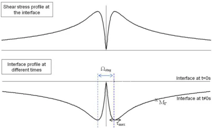
According to the erosion law in Eq. (5), the displacement of a point at the interface depends only on the shear stress exerted by the fluid on the material at this point. In the case of a flow normal to the surface of the soil, the mean shear stress is null at the stagnation point, then increases up to its maximum and then decreases again by receding from the stagnation zone. The implementation of the erosion law as it is should progressively lead to a geometric singularity of the erosion pattern in the stagnation zone, as shown schematically in Figure 1 where the shear stress profile is also plotted.
In the case of erosion caused by a turbulent jet flow, one finds no singularity in practice. On the contrary, a symmetric cup-shape with the maximum depth at the jet centerline is observed.
The inhomogeneity of a real soil can explain the absence of a non-eroded soil peak at the jet centerline. The addition of a flow mechanical quantity in the erosion law could also lead to the smoothing of the theoretical non eroded peak. In addition, the fluctuations of instantaneous turbulence quantities in the stagnation area of the jet, as well as the pulse of the jet in 3-D geometry, may explain this smoothing of the peak of non-eroded soil. Hadziabdic and Hanjalic [22] displayed fluctuations of the location of the stagnation point for an impinging jet, but the amplitude of the stagnation point displacement cannot be found directly from this study for our problem configuration. More work is needed to precisely model these effects and integrate them in a reliable erosion law; but this subject is outside the scope of the present study. Therefore, for the sake of simplicity, we use the following simplified model as a first step: on Γ (20) where is the stagnation zone of the jet flow defined as in Figure 1, and , the
maximum shear stress.
The procedure for shifting the interface nodes is the following: extraction of the calculation data at the interface, determination of the erosion time step in agreement with a CFL (Courant Friedrichs Lewy) type condition applicable to Eq. (16), ordering of the nodes composing the fluid/material interface, determination of the shift associated with each node by a first order Euler type graph and reordering and shifting of the nodes. The time step is chosen so that the largest displacement of the interface cannot reach more than a tenth peak of the smallest interface cell size, to ensure a very good stability of the erosion model.
4. Model validation of a jet impinging on a non erodible wall
4.1. Geometry and limit conditions of the flow
The geometry of the computation domain is 2D axisymmetric, representative of the configuration developed by Hanson et al. [16], as presented in Figure 2.
The water flow enters the controlled pressure injection cylinder, passes through a nozzle and impinges on the surface of the material. The water is discharged through lateral orifices, in agreement with the axisymmetric geometry. The free surface corresponding in reality to overtopping is modelled symmetrically. The condition of symmetry is a null flux condition, whatever the variable considered, with null mean velocity and null gradients for the shear stress. A sliding condition is imposed, thus we could also consider a frictionless wall.
One should consider the free surface using VOF free surface models, but this would uselessly increase the complexity and the computational time, whereas the free surface is relatively far from the core of the problem and should have only a very slight effect on the erosion kinetics. A differential pressure of 3x10⁴ Pa is imposed. The distance separating the 6.35 mm diameter nozzle from the water/material interface is 146.5 mm.
4.2. Mesh density
The first point to be validated concerns the independence of the results with respect to meshing. Several factors have to be taken into account: the mesh fineness of the nozzle and the surface of impingement between the two elements. The influence of the rest of the mesh
on the modelling results is lower, apart from the outlet mesh density, due to possible convergence problems.
Table 1 groups the characteristics of the different meshes tested: the number of mesh nodes at the outlet orifice varies from 10 to 100 and the limit layer at the water/soil interface from 350 to 7,000, for a total number of cells ranging from about 27,000 to nearly 1,200,000 elements. Meshes A to M are characterised by the variation of the number of mesh nodes at the jet outlet orifice. Meshes N to S present a number of mesh nodes on the sublayer which varies as a function of the number of mesh nodes at the orifice of the jet outlet. Meshes T, U and V differ by the number of mesh nodes in the tank as a function of the two other parameters. This sensitivity analysis was performed using solely the turbulence model.
The results obtained for the shear stress and the total pressure at the water/soil interface are shown in Figures 3a and 3b. They indicate that, regarding the sensitivity study of mesh density at the outlet orifice, the shear stress curves oscillate around the results provided by meshes K, L and M for a very dense mesh at the nozzle. The results are independent of mesh density to within 5%, taking into account a mesh density close to 30 cells at the outlet orifice. The independence of the results with respect to the mesh density of the water tank was obtained with the first mesh tested. Varying the number of cells in the tank had less effect in this case.
Increasing the number of cells at the water/soil interface leads to a reduction and a shift of the maximum stress to the left of the maximum peak obtained for a mesh of 350 cells in the sublayer. The reduction of the maximum pressure and shear stress is greater than 5%. The width of the pressure curve at mid-height is much lower in the case of a dense mesh at the interface.
In the case of meshes composed of 350 elements at the interface, we obtain y+9. For those with 3,000 elements at the interface, y+1 and for 7,000 elements, we obtained y+0.5. In the three cases, and whatever the mesh considered, the turbulent Reynolds number at the wall remained less than 200 and the one-equation model of Wolfshtein [17] can therefore be used to solve the flow at the wall.
However, the similarity of the results given by meshes P, Q, R and S permits deducing that, for this geometry, the precision of the results is independent of meshing as from 0.9<y+<1 in the near wall zone. The increase in computation time can nonetheless quickly become a severe handicap as mesh density at the interface increases. The appearance of potential instabilities can be observed for mesh elements whose size is too small.
The erosion law given in Eq. (19) relies only on the influence of the shear stress, using all the results obtained above and shown in Figure 3a. It appears that mesh P is the most suitable, since it combines independence of the results from the mesh, whatever the mesh considered, with an optimal number of cells in order to reduce the computing time. However, the large number of cells on the water/soil interface allows only a very short erosion time step and the oscillations of the shear stress curve are non negligible. Therefore priority will be given to the use of mesh I.
4.3. Influence of the turbulence model
This study of the turbulence model influence on the numerical results was performed by comparing the results of , and RSM turbulence models with results from literature: Beltaos et al. [23], Hanson et al. [24], Looney et al. [11], Poreh et al. [25], Viegas et al. [26]. The parameters governing the flow are the velocity on the jet centerline, the pressure field and the shear stress at the interface.
The velocity of the flow at the outlet orifice U can be compared to the Hanson et al. [24] 0
formula, with ΔH being the height of the water column and g gravitational acceleration:
0 = 2 Δ
U g H (20)
The potential core, i.e. the core forming immediately at the outlet of the jet, is characterised by a velocity on the jet centerline which remains constant and equal to U . The length of the 0
potential core, denoted l , has been the subject of many studies, especially those of Beltaos et al. [23], Looney et al. [11]. Thus, with d0 the diameter of the outlet orifice, the most
commonly used empirical formula reads:
0
6.2
l≈ d (21)
The auto-similarity of non-impinging jets has also been the subject of much research: Tritton [19], Hanson et al. [24]. Let us denote the normal component of the velocity at any point of the median axis of the jet as U z
( )
, with z being the ordinate of the point considered in the geometrical reference presented in Figure 2. The distribution of the velocity outside the potential core at the jet centerline is then:( )
0 ifl
U z U z l z
= > (22)
Beltaos et al. [23] and Hanson [24] gave empirically the value of the pressure peak on the impingement surface at the jet centerline, denoted Pmax, and the distribution of pressure on the
flat, non erodible surface, P r
( )
. Here r denotes the distance to the jet centerline and z the 0distance separating the height of the jet outlet and the interface:
2 0 max 2 0 0 ( / ) = wU P C z d
ρ
(23)( )
2 0 114( / ) max r z P r e P − = (24)The value of coefficient C found experimentally by Beltaos et al. [23] in air with a planar jet is 25.0. Poreh et al. [25] obtained 30.2 in water whereas Hanson et al. [24] obtained 27.8 in water with a circular jet.
Beltaos et al. [23] give the following empirical expressions for the maximum shear stress on the impingement surface and the radial distribution of shear stress for a range of distances to the jet centerline less than r<0 22. z0:
2 0 max 2 0 0 0.16 ( / ) wU z d
ρ
τ
= (25)(
)
2 0 2 0 114( / ) 114( / ) 0 max 0 ( ) 1 0.18 9.43 / / r z r z r e r z e r zτ
τ
− − − = − (26)Viegas et al. [26] give an empirical formulation of the shear stress distribution for a range of distances to the median axis of the jet higher than r>0 22. z0 :
(
)
0.078 0 0.878 0.256 0 0 max ( ) 0.67 / d r d r zτ
τ
− − = (27)Hanson et al. [24] established empirical formulas of the shear stress distribution and the maximum shear stress at the interface:
(
)
0.6 0 7.68( / ) 0 max ( ) 66.5 / r z r r z eτ
τ
= − (28)0.74 2 0 max 2 0 0 0.56 ( / ) wU z d
ρ
τ
= (29)Phares et al. [27] give an empirical formula of the maximum shear stress at the interface, with
the Reynolds number of the flow at the jet outlet orifice:
0 2 2 0.5 0 max 0 0 44.6 w e z U R d
τ
ρ
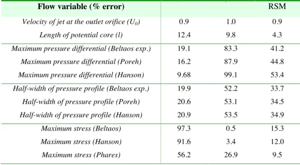
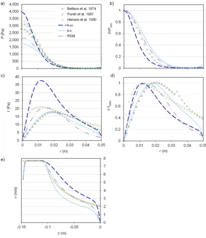
− − = (30)Table 2 reports the percentage errors obtained by comparing the results of different turbulence models with results from the literature. Figure 4 shows the comparison of numerical and experimental results.
The results for pressure are shown in Figures 4a and 4b. It can be seen that the model presents results that fit better with the empirical formulas in the literature than the RSM model, with a relative average error of 20% and 37% respectively. As for the model, it is far below the maximal pressures obtained in the literature, with an error ranging from 65 to 100% according to the empirical model considered. The results on the half length of the pressure profile show the same trend. On the contrary, the results on the maximum shear stress are closer to the results in the literature in the case of the and RSM models, to within 10 and 12% respectively, and are very far from the empirical formulas in the case of the model, with an error of 82% (Figures 4c and 4d). Regarding the velocity of the flow close to the jet nozzle (Figure 4e) the results obtained for the three turbulence models are in good agreement with the empirical results in the literature, especially the RSM model which presents an error of about 3%.
Globally, the RSM model comes closest to the empirical results in the literature. The model presents the results closest to the results in the literature for flow velocity and pressure. The model presents the results closest to those in the literature for shear stress. As expected, we infer that the turbulence model is more adapted to the numerical modelling of jets than the model. However, the shear stress on the interface obtained with the turbulence model is closer to bibliographic data.
The three types of turbulence models, , and RSM, were considered for modelling the erosion of a cohesive soil by a turbulent flow. However, the difficulty of implementing the RSM model made it difficult to use due to the successive remeshing of the calculation domain. Despite its accuracy, the RSM model presents a considerable degree of instability. Therefore its use is not adapted to successive remeshings. A quite good convergence of the RSM is ensured by initialising the model with results. Between each remeshing, a
numerical model must be carried out; the RSM should then be used. This leads to a
considerable increase of the calculation time and the convergence of the erosion model is still not guaranteed. Therefore, only the results obtained for the and turbulence models are presented in the following paragraphs.
5. Validation of the model with erosion
5.1. The results of the numerical model with erosion
The characteristics of the soil, obtained using the model of Hanson et al. [16], are
5
1 10 m².s/kg d
k = × − and
τ
c =11 Pa. These parameters are standard values of results obtained for a soil in the classification of Hanson et al. [16]. In addition to this standard case, a parametric study of the critical shear stress and the erosion coefficient will be presented inorder to better understand the influence of these parameters on the erosion law and on the results of our numerical modelling.
Given the considerable computing times generated by this type of numerical simulation, a coarser mesh than mesh I was used for this study, otherwise two months of calculation on a cluster of 8 CPUs with Intel Xeon EMT64 3.2 GHz dual processors would have been required. Mesh D was used for the model without erosion, leading to an error of 15% in comparison to the results obtained with the denser meshes tested, but requiring only half the calculation time.
To illustrate the evolution of both the hydrodynamics and soil’s boundary, Figure 5 shows the evolution of the fluid velocity field and the geometry of the soil/water interface as a function of erosion times obtained with the and turbulence models.
Let z∞ denote the distance separating the height of the jet outlet and the soil’s interface at the median axis of the jet, at the end of the erosion process (at time t= +∞). The master equations of the semi-empirical model of Hanson et al. [16] can be rewritten as follows:
(31) and with (32) with (33)
with a friction coefficient Cf=0.00416 determined empirically and the reference shear
stress.
Figure 6 illustrates the evolution of the soil/water interface as a function of erosion time, in the case of models (a) and (b). In conformity with the results obtained when comparing the turbulence models, where the shear stress was much lower in the case of the
turbulence model than in the case of the model, the erosion process follows the
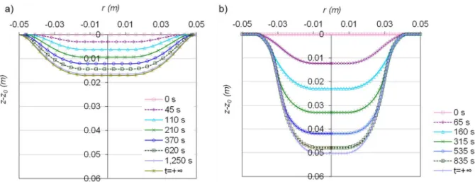
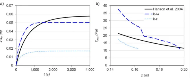
same trend. At the end of the erosion process, when the shear stress becomes lower than the critical shear stress at every point of the interface and the soil is no longer subject to erosion, the maximum scouring with model is about 1.74 cm whereas it is about 5.03 cm with the model.
The portion of the water/soil interface affected by the erosion is larger with the model, in line with the observations of Figure 4d, with a larger half-width of the shear stress profile for the model. For the moment, we did not implement a limit to the interface slope. Figure 7a presents the evolution of scouring depth a function of erosion time for the two turbulence models tested, in comparison to the results of the erosion model of Hanson et al. [16]. For the study without erosion, the model presents a profile and maximum shear stress close to the literature results. However, when modelling erosion, the comparison of maximum scouring as a function of erosion time shows better correspondence between the numerical results and the semi-empirical model, as illustrated in Figure 7a. The relative error on the final maximum scouring depth, between the numerical and semi-empirical results is 17.7% with the model whereas it reaches 71.6% for the one.
Figure 7b shows the evolution of the maximum shear stress as a function of scouring depth at different erosion times for and models in comparison to the results given by the empirical model. For the evolution of the shear stress as a function of time, the semi-empirical model proposes the following expression for the median axis of the jet:
(34)
We observe Figure 7b that the model is initially rather close to the empirical model whereas the model presents a high percentage error. The end of the curve shows an inversion of the trend when increasing erosion time. The slope of the maximum shear stress curve as a function of maximum scouring is much higher in the case of the model than for the model, thereby leading to a rapid stop of the erosion process. With the model, the slope of the curve of the maximum tangential stress curve as a function of scouring depth is also very high. The error between the results given by the model and those given by the semi-empirical model decreases as erosion time increases. A clear break in the curve in the case of the model can be seen for a scouring depth of around 2 cm. Detailed observation of the flow parameters at different erosion times is carried out hereafter to understand this phenomenon.
Figure 8 shows the evolution of the different flow variables as a function of erosion time: the velocity field on the median axis of the jet, the shear stress and static pressure on the soil/water interface. Generally, these curves fluctuate more than those for a jet without erosion, obtained using the turbulence model. After a certain time of erosion, the pressures at the extremities of the interface become negative, prefiguring the appearance of recirculation zones within the flow. As shown in Figure 8a, the shape of the shear stress at the interface clearly changes as from the first remeshing of the entire zone affected by meshing deformation. Regarding the other flow variables, the velocity profile at the median axis of the jet (cf. Figure 8b) and static pressure at the interface (cf. Figure 8c), a significant increase of the maxima between the state with no erosion and the first remeshing is also observed. Then, whatever the flow variable considered, the values fall until stabilising at the final equilibrium regime when the erosion process ceases. There is an obvious and sudden fall in all the flow variables between the curves at 106.4 s and 130.4 s, a drop corresponding to that observed in Figure 7b.
Figure 9 shows the pressure profiles obtained at different erosion times, the start and end of the erosion process, and at t 106 sand t 130 s, obtained with turbulence models and , with the former shown above the latter. The upper part of Figure 9 shows the pressure profiles obtained with the model at different erosion times: the start and end of the erosion process, and at and . Between the last two profiles a brutal fall of all the flow variables is observed. The scale represented corresponds to 10% of the full spectrum of the pressure field in the flow. The corresponding graphs clearly show the appearance of recirculation zones above the convexity zone of the soil/water interface between times 106 s and 130 s, with the model. A change of flow regime occurs at a scouring depth of about 2 cm. With the model, the evolution of the pressure field presented in the lower part of Figure 9 reveals a flow regime similar to that found with the
model for the same depths, except for the fact that lateral diffusion of the jet is larger
with the model. The jet therefore impinges on the soil/water interface with less power, and whatever the depth of the cavity it is seen that the flow at the outlet of the cavity remains at a tangent to the horizontal plane. Conversely, in the framework of the model, the impingement of the jet at the bottom of the cavity with a larger power permits the resurgence of the flow in an almost vertical direction at the outlet of the cavity, once the depth of the latter exceeds approximately 2 cm. As is widely documented, the does not perform very well for turbulent boundary layer flows with streamwise pressure gradient or wall curvature, for which the is known to perform much better [28,29]. This probably explains what is observed on Figure 9, even though a more specific study would be required
to analyze these results in more detail. This specific study could include, for instance, the comparison of standard and SST results.
5.2. Parametric study of the erosion coefficient and critical shear stress
A parametric study of the influence of critical shear stress and erosion coefficient on the evolution of scouring depth as a function of erosion time was carried out using the turbulence model. For an unchanged erosion coefficient of , the influence of the critical shear stress is presented for
τ
c equal to 0, 5, 9, 13 and 20 Pa, in addition to the initial caseτ
c=11 Pa, in Figure 10a. The influence of the erosion coefficient is presented ford
k equal to 2 10 and 5×10 m².s/kg× -5 -6 in Figure 10b, for a constant
τ
c =11 Pa. The cases 9 Pac
τ
= ,kd =5×10 m².s/kg-6 andτ
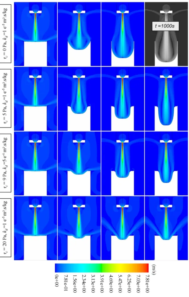
c =9 Pa, kd =3×10 m².s/kg-6 were also modelled and plotted in Figure 10b. As can be seen in Figure 10a, a differential critical shear stress of only 2 Pa, i.e. about 20% in relative value, leads to a difference of more than 8 mm in the maximum scouring depth, i.e. a relative difference of about 15%. Likewise, cf. Figure 10b, a difference of 50% on the erosion coefficient could lead to a difference of almost 50% over the time required to reach equilibrium state. The parametric study demonstrates that the results obtained by numerical modelling agree quite well with results obtained with the semi-empirical model. A considerable error on one of the parameters, critical shear stress or erosion coefficient, would give rise to considerable differences between the numerical and semi-empirical results, on the evolution of the scouring depth as a function of time.Figure 11 shows the magnitude of the velocity as well as the shape of the soil/water interface profile obtained for these different sets of parameters at times: 6 s, 200 s, 600 s, 15,000 s, and in the final state. The erosion figures and velocity fields show the influence of the critical shear stress and erosion coefficient on the shape of the eroded surface and on the characteristics of the flow. In line with the observations made on the direction of the flow as a function of cavity depth, when the depth of the cavity formed is close to 2 cm, the flow at the outlet of the cavity changes quickly from a tangential direction to one perpendicular to axis r. This transient phase is shown clearly by the two final images corresponding to the last combination of parameters tested,
τ
c =20 Pa,kd =1×10 m².s/kg-5 . The variation of the erosion coefficient only appears to affect the kinetics to reach the final state. It is necessary to check that z∞ only depends on the critical stress, as suggested by the images corresponding to the numerical simulations performed with the following sets of parameters:τ
c=9 Pa withd
k equal to 3 10× -6, 5 10× -6 and 1 10 m².s/kg× -5 or
τ
c =11 Pa with k equal to d 5 10× -6,-5
1 10 × and 2 10 m².s/kg× -5 . When the erosion process stops, the erosion figures corresponding to the same
τ
c are indeed strictly alike. Consequently k has no influence on dthe shape of the final erosion configuration.
The variation of the critical shear stress also affects the shape of the eroded area as well as the maximum scouring depth and the kinetics. For a null stress, the entire surface of the material is eroded; in the last two images of case
τ
c =0 Pa,kd = ×1 10 m².s/kg-5 the walls of the mould, with a thickness of 2 mm, became apparent. Erosion stops only when all the soil contained in the mould has been eroded, but, given the long computing times involved, the numerical simulation was stopped at t=1,000 s, thus the maximum distance reached by the erosion is therefore only 1 cm from the bottom of the mould. The higher the critical shear stress, the more the zone affected by erosion decreases with, notably, a decrease of the maximum depth reached. Less material is eroded and the cavity formed is narrower and lessdeep. Figure 10a also provides a good illustration of the differences observed on the scouring depth and also on the influence of the critical shear stress on the erosion kinetics. The higher the critical shear stress, the shorter the time required to reach the moment when the erosion process stops. However, Figure 10b shows that, for the same erosion coefficient and similar threshold stresses, such that
τ
c =9 Pa andτ
c =11 Pa, the times required to reach equilibrium are almost the same whereas in the caseτ
c =9 Pa a variation of only 2×10 m².s/kg on -6 k dleads to a difference of over 1,500 s in the time required to reach equilibrium. Thus, initially, the erosion coefficient governs the kinetics of the process, although the time required to reach stable flow is not independent of the critical shear stress. Thus, at t1/ 2, the time at which the erosion depth reaches half of z∞− , it is necessary to check that: z0
( )
cz∞ = f
τ
(35)(
)
1/ 2 d c
t =g k ,
τ
(36)with f and g being functions whose curves are plotted in Figure 12.
Figure 12a shows the time necessary for the erosion process to reach half the maximum scouring reached when the erosion process stops, as a function of the erosion coefficient, for
11 Pa =
c
τ
. Figure 12b shows scouring as a function of critical shear stress for-5
1 10 m².s/kg = ×
d
k . Figure 12c presents the time required for the erosion process to reach half the maximum scouring reached when the erosion process stops, as a function of the critical shear stress, forkd = ×1 10 m².s/kg-5 . From Eq. (31), the semi-empirical model gives:
(37) with (38)
Figure 12 compares the numerical results found during this parametric study with those obtained with the semi-empirical model. Before the start of the erosion process, the shear stress exerted by the fluid on the material is much lower in the case of the semi-empirical model than for the numerical model. This point explains why the semi-empirical curve starts at much lower critical shear stresses than the numerical model, cf. Figure 12b. Nonetheless, the semi-empirical and numerical curves remain quite close. As for the total duration of the erosion process as a function of the erosion coefficient, cf. Figure 12a, apart from a quite considerable shift, the shapes of the semi-empirical and numerical curves remain similar. The lower the values of k are, the higher the error between the numerical and semi-empirical d
results will be. The curve representing the influence of the critical shear stress on the erosion kinetics, cf. Figure 12c, is also very close to the results of the semi-empirical model. As with the values of k , the lower the values of d
τ
c, the higher the error between the numerical and semi-empirical results.6. Discussion
The main subject of discussion related to this study concerns the significant differences obtained for the results given by the and turbulence models.
For jets impinging on a wall with no erosion, since the type models tend to become over-diffusive, it seems normal that this type of model attenuates the flow variables at the interface. Furthermore, the study on the influence of the turbulence model shows that
Reynolds Stress Model type model provides results very close to those in the literature. For all the flow quantities considered, these results fall between those given by the model and those given by the the model. However, it was not possible, in the present state of this study, to obtain the convergence of the RSM when modelling erosion. A small number of successive remeshing steps are sufficient to cause divergence of the numerical computation. The results given by the and models nonetheless complement each other.
To our knowledge, very few studies have focused on the distribution of shear stress imposed on a wall by an impinging jet flow. However, the results we found in the literature show that the turbulence model gives the best results on the maximum shear stress on the wall for a flat interface. Nonetheless, the results of the model with erosion show an inversion of this trend in favour of the model. Unlike the , the turbulence model does not perform very well for turbulent boundary layer flows with streamwise pressure gradient or wall curvature. This could explain the inversion of this trend. It is also difficult to estimate the error margin to be taken into account on the semi-empirical results found in the literature. Given the current state of progress of this study, it is not possible to conclude with certainty as to the pertinence of the and type models. But whatever the case, the orders of magnitude obtained for both models tested correspond quite well to the semi-empirical model. The results obtained herein show that the soil erosion corresponding to JET tests presents a subtle balance between the pressure in the jet flow and the shear stress generated by the flow established on the surface of the soil. Further analysis is obviously required to better understand the physical mechanisms involved in impinging jet erosion, in order to derive a specific erosion law for that particular situation, and generalize the usual erosion laws which were derived for tangential flow erosion.
7. Conclusion
The objective of this work was to build a pertinent numerical model of the erosion of a cohesive soil by an impinging turbulent jet flow.
The modelling method developed is a combined Euler-Lagrange method, involving a turbulent Navier-Stokes model of the flow with adaptive remeshing. A Lagrangian algorithm was implemented for the displacement of the interface to model the erosion of the soil/water interface. The hypotheses of slow erosion and diluted flow made it possible to perform loose-coupling sequential modelling of the erosion.
The erosion law was adapted successfully to take into account the stagnation point, in the specific case of an impinging jet. A simple model was made of the spatial fluctuations of turbulent structures in the impingement zone, which probably explains the smoothing of the peak of the theoretical non eroded soil at the stagnation point of the jet flow.
The results obtained by the modelling method developed were first validated for a flat surface configuration. The study of the influence of the turbulence model on the modelling results without erosion led to the conclusion that, globally, the RSM model gave the best correspondence with the results in the literature. However, it was difficult to implement and could not be used for modelling erosion. The k-
ε
and k-ω
type turbulence models appeared complementary: the k-ε
and k-ω
models presented the results closest to the results in theliterature on shear stress and pressure respectively. The choice of using both models for the numerical modelling of the erosion of a cohesive soil by an impinging jet was performed. The results obtained for numerical modelling with erosion show that the calculations based on a k-
ω
turbulence model are closer to the semi-empirical results obtained by the model of Hanson and al. [16]. This study highlighted the appearance of recirculation zones and a change in orientation of flow at the outlet of the cavity, when the convexity of the soil/waterinterface becomes significant in the case of the k-
ω
turbulence model. The numerical results obtained with the k-ε
type turbulence model remain consistent with the orders of magnitude of the results given by the semi-empirical model.8. Acknowledgements
This study was carried out with the support of the Centre d’Ingénierie Hydraulique of EDF and geophyConsult. The authors of this publication would like to extend special thanks to Mrs
Patrick Pinettes (geophyConsult), Jean-Robert Courivaud (EDF) and Jean-Jacques Fry (EDF)
for their support and confidence. This work was also funded by the French National Research Agency (ANR) through the COSINUS program (project CARPEINTER No. ANR-08-COSI-002).
9. References
[1] I. Vardoulakis, M. Stavropoulou, P. Papanastasiou, Hydromechanical aspects of sand production problem, Transport in Porous Media, 22 (1996) 225-244.
[2] M. Ouriemi, P. Aussillous, M. Médale, Y. Peysson, E. Guazzelli, Determination of the critical Shields number for particle erosion in laminar flow, Physics of Fluids, 19 (6) (2007) 061706.
[3] O. Brivois, S. Bonelli, R. Borghi, Soil erosion in the boundary layer flow along a slope : a theoretical study, European Journal of Mechanics B/Fluids, 26 (2007) 707-719.
[4] D. Lachouette, F. Golay, S. Bonelli, One-dimensional modelling of piping flow erosion, Comptes Rendus de Mécanique, 336 (2008) 731-736.
[5] F. Golay, D. Lachouette, S. Bonelli, P. Seppecher, Numerical modelling of interfacial soil erosion with viscous incompressible flows, Computer Methods in Applied Mechanics and Engineering, 200 (2011) 383-391.
[6] S. Osher, J.A. Sethian, Fronts propagating with curvature dependent speed: algorithms based on Hamilton-Jacobi formulation, Journal of Computational Physics, 79 (1988) 12-49. [7] S. Bonelli, O. Brivois, The scaling law in the hole erosion test with a constant pressure drop, International Journal for Numerical and Analytical Methods in Geomechanics, 32 (2008) 1573-1595.
[8] B.E. Launder, D.B. Spalding, Lectures in mathematical models of turbulence, Academic Press London, 1972.
[9] D.C. Wilcox, Turbulence modelling for CFD, DCW Industries, La Canada, California, 1998.
[10] B.E. Launder, G.J. Reece, W. Rodi, Progress in the development of a Reynolds-stress turbulence closure, Journal of Fluid Mechanics, 68 (3) (1975) 537–566.
[11] M.K. Looney, J.J. Walsh, Mean flow and turbulent characteristics of free and impinging jet flow, Journal of Fluid Mechanics, 147 (1984) 397-429.
[12] T.J. Craft, L.J.W. Graham, B.E. Launder, Impinging jet studies for turbulence model assessment II An examination of the performance of four turbulence models, International Journal of Heat and Mass Transfer, 36 (10) (1993) 2685-2697.
[13] J.E. Jaramillo, C.D. Pérez-Segarra, I. Rodriguez, A. Olivia, Numerical study of plane and round impinging jets using RANS models, Numerical Heat Transfer, 54 (2008) 213-237.