HAL Id: tel-00978589
https://tel.archives-ouvertes.fr/tel-00978589
Submitted on 14 Apr 2014HAL is a multi-disciplinary open access archive for the deposit and dissemination of sci-entific research documents, whether they are pub-lished or not. The documents may come from teaching and research institutions in France or abroad, or from public or private research centers.
L’archive ouverte pluridisciplinaire HAL, est destinée au dépôt et à la diffusion de documents scientifiques de niveau recherche, publiés ou non, émanant des établissements d’enseignement et de recherche français ou étrangers, des laboratoires publics ou privés.
Florian Mercier
To cite this version:
Florian Mercier. NUMERICAL MODELLING OF EROSION OF A COHESIVE SOIL BY A TUR-BULENT FLOW. Fluids mechanics [physics.class-ph]. Aix-Marseille Université, 2013. English. �tel-00978589�
U
NIVERSITY OF
A
IX
-M
ARSEILLE
D
OCTORAL
S
CHOOL
:
E
NGINEERING
S
CIENCES
N
UMERICAL
M
ODELLING OF
E
ROSION OF A
C
OHESIVE
S
OIL BY A
T
URBULENT
F
LOW
PhD Thesis presented to obtain the grade of
D
OCTOR OF THE
U
NIVERSITY OF
A
IX
-M
ARSEILLE
S
PECIALITY
:
M
ECHANICS AND
P
HYSICS OF
F
LUIDS
by
Fabienne M
ERCIER
Defended publicly on 11 June 2013
Before a jury composed of
Fabien A
NSELMETIRPHE
Co-thesis supervisor
Eric B
ARTHÉLÉMYLEGI
Examiner
Stéphane B
ONELLIIRSTEA
Thesis supervisor
Roland B
ORGHIECM
Examiner
Jean-Robert C
OURIVAUDEDF-CIH
Guest
Jean-Jacques F
RYEDF-CIH
Guest
Frédéric G
OLAYIMATH
Examiner
Philippe G
ONDRETFAST
Reporter
Didier M
AROTGeM
Reporter
Marc M
ÉDALEIUSTI
Examiner
ACKNOWLEDGEMENTS
I would first like to thank my thesis supervisors, Stéphane BONELLI and Fabien ANSELMET. Their sceintific expertise and the knowledge they provided allowed me to carry out this complex study at the crossroads of several disciplines in an pleasant atmosphere. I would also like to thank the manager of geophyConsult, the company involved in the CIFRE funding (Industrial Research Convention: PhD conducted with an industrial partnership), Patrick PINETTES, for his technical and scientific competences, and for his constant moral support.
The organisation of this CIFRE thesis would certainly never have succeeded without the contribution of Jean-Jacques FRY. Thank you for all the advice that you gave me at the beginning of this adventure and afterwards. I also thank Jean-Robert COURIVAUD, first for the funding given by EDF for this thesis and for his continuous follow-up of my work and his scientific contribution to this study.
I would also like to thank Laurent PEYRAS for his active contribution to the organisation of this thesis and his support throughout this study. My thanks also go to Pierre PHILIPPE, Frédéric GOLAY and Roland BORGHI for their availability and encouragement.
I thank the members of the jury for the attention they have given to my work and the resulting positive feedback. Your questions and remarks contributed to the subsequent direction taken for work performed in the framework of this thesis.
I thank the entire team of the Laboratoire de Mécanique des Sols de l’Unité des Ouvrages hydrauliques et Hydrologie of IRSTEA. I thank Alain BERNARD and Nadia BENAHMED for their perspicacious advice. I thank Faustine BYRON, Yves GREMEAUX and Guillaume NUNES for their technical assistance, their good humour and all the good times we spent together. I thank my fellow PhD students who contributed to the good atmosphere in the team on a daily basis: Caroline ZANETTI, Mohammed ARIS, Félix BONNET, Kien NGUYEN, Jeff NGOMA and Zhenzhen LIU. I am also very grateful to my office colleagues, Damien LACHOUETTE, Marc VUILLET, Ismail FAKHFAKH, Marika BOUTRY and particularly Li-Hua LUU, who was kind enough to read this thesis. My thanks also go to the assistants of the unit and the group: Martine SYLVESTRE, Monique COSTET, Christiane BONNET and Dominique BREIL. I spare a thought for all the other people in the IRSTEA team that I have frequented during different sports and summer activities.
I especially thank the members of the computer department of the IRSTEA centre of Aix-en-Provence: Alain GERARD, Mathieu LESTRADE and Etienne BLANC. I would also like to thank Vincent CHEVALLEREAU and Gérard DELANCE as well as the whole team of the IRSTEA calculation unit, for the resources that they implemented for me so I could carry out my scientific calculation projects. I also extend my thanks to the Information Systems Division (DSI) of IRSTEA.
I am grateful to my colleagues of geophyConsult : Cyril GUIDOUX, Rémi BEGIN, Olivier MARIN and above all Clément MORAS, for all the JET tests he performed with me or for my research.
I am also grateful to the IRPHE team, especially Muriel AMIELH, and to Pascal CAMPION of ED353 for his availability and efficiency.
And above all, I am especially grateful to my family and friends without whom none of this would have been possible.
TABLE OF CONTENTS
Figure captions ... 9
Table captions ... 15
Nomenclature ... 17
Introduction ... 23
Chapter 1. State of the art ... 27
1.1 Erosion in hydraulic structures ... 27
1.1.1 Context ... 27
1.1.1.1 Erosion at the scale of the structure... 27
1.1.1.2 Estimation of soil erodibility ... 29
1.1.1.3 Erosion parameters ... 29
1.1.2 HET and JET erosion tests ... 30
1.1.2.1 The Hole Erosion Test ... 30
1.1.2.2 The Jet Erosion Test ... 33
1.1.3 Erosion laws ... 35
1.1.3.1 Rate of soil removal ... 35
1.1.3.2 Determination of critical shear stress ... 39
1.1.3.3 Correlation of erosion coefficient and critical shear stress ... 41
1.2 Numerical modelling of erosion ... 42
1.2.1 Context ... 42
1.2.1.1 Erosion of granular soils and cohesive soils ... 42
1.2.1.2 Different approaches to model interfaces ... 43
1.2.2 Biphasic and triphasic models ... 44
1.2.2.1 The approach of Papamichos and Vardoulakis (2005) ... 44
1.2.2.2 The approach of Ouriemi et al. 2009 ... 45
1.2.3 Singular interface ... 46
1.3 Conclusions on the state of the art ... 48
Chapter 2. Modelling method ... 51
2.1 Hypotheses ... 51
2.1.1 Single phase modelling and slow erosion kinetics ... 51
2.1.2 Analysis of orders of magnitude ... 52
2.2 Flow modelling ... 53
2.2.1 RANS modelling and the closure problem ... 53
2.2.1.1 Navier-Stokes Equations ... 53
2.2.1.2 Resolution by DNS or LES ... 53
2.2.1.3 Choice of RANS models ... 53
2.2.2 Turbulence models ... 54
2.2.2.1 Eddy viscosity models ... 54
2.3 Erosion modelling ... 56
2.3.1 Classical erosion law ... 56
2.3.1.1 Definition of the eroded mass flux ... 56
2.3.1.2 Shear stress ... 56
2.3.2 The standard erosion law adapted to impinging jets ... 57
2.3.2.1 Geometric singularity induced by the erosion law ... 57
2.3.2.2 Smoothing of the non eroded soil peak ... 58
2.3.2.3 Adaptation of the erosion law ... 60
2.4 Numerical model ... 61
2.4.1 Global numerical method ... 61
2.4.2 Flow discretization ... 62
2.4.2.1 Solution of Navier-Stokes equations ... 62
2.4.2.2 Wall laws ... 63
2.4.2.3 Taking roughness into account ... 65
2.4.3 Updating the position of the interface ... 66
2.4.3.1 Interface displacement code ... 66
2.4.3.2 Remeshing ... 68
2.5 Conclusions on the modelling method ... 71
Chapter 3. Results obtained on impinging flows ... 73
3.1 Independency of results regarding mesh density and turbulence models ... 73
3.1.1 Independency of results in relation to the meshing ... 74
3.1.2 Influence of the turbulence model ... 77
3.2 Erosion modelling ... 81
3.2.1 Comparison of results of the semi-empirical model ... 81
3.2.2 Study of the sensitivity of the model to erosion parameters ... 87
3.2.3 Discussion ... 93
3.3 Validation of the JET interpretation model ... 95
3.3.1 Characterization of the soils tested ... 95
3.3.2 JET modelling results ... 101
3.3.3 Discussion ... 107
3.4 Conclusions on the application to jet flows ... 108
Chapter 4. Results obtained on tangential flows ... 111
4.1 Validation of the numerical model in a 2D Poiseuille flow configuration ... 111
4.1.1 Theoretical solution ... 111
4.1.2 Numerical results ... 112
4.2 Concentrated leak erosion in turbulent flow ... 114
4.2.1 Independence from meshing and turbulence models ... 115
4.2.1.1 Independence of results from mesh density ... 115
TABLE OF CONTENTS
4.2.2 Results with erosion ... 120
4.2.3 Study of the model’s sensitivity to erosion parameters ... 126
4.2.4 Discussion ... 129
4.3 Modelling the HETs ... 130
4.3.1 Characterisation of the soils modelled ... 130
4.3.2 HET modelling results ... 134
4.3.3 Discussion ... 142
4.4 Conclusions of the application to piping flows ... 143
Chapter 5. Study of the erosion law ... 145
5.1 Differences between JET and HET for erosion parameters ... 145
5.1.1 Experimental and literature data ... 145
5.1.2 Dispersion of results ... 149
5.1.3 Influence of flow parameters ... 151
5.2 Variables susceptible to influence erosion ... 153
5.2.1 Possible explanations for JET and HET differences? ... 153
5.2.2 Flow signature ... 155
5.2.2.1 Stresses and forces exerted by the flow on the plane ... 158
5.2.2.2 Pressure gradient ... 160
5.2.2.3 Turbulence variables ... 162
5.2.3 Flow variables susceptible to influence erosion ... 164
5.3 Paths for developing the erosion law ... 166
5.3.1 Flow variables of the JET and HETs ... 166
5.3.2 Taking fluctuations into account in the stagnation region ... 171
5.3.3 Taking into account the pressure gradient in the erosion law ... 172
5.4 Conclusions on the study of the erosion law ... 173
Conclusion ... 175
Outlook for further research ... 179
FIGURE CAPTIONS
Figure 1.1. Breach caused by flooding of the Virdourle river in 2002 (left) and breach of
Teton Dam, 1976 (right).
Figure 1.2. Simplified schematic diagram of the Hole Erosion Test. Figure 1.3. Photograph of the Hole Erosion Test experimental device.
Figure 1.4. Grouping of HET test results for a flow rate imposed on the master curve defined
by equation (1.7) of [Bonelli et al. 2012].
Figure 1.5. Simplified schematic diagram of the Jet Erosion Test.
Figure 1.6. Photograph of experimental JET device in the laboratory and in-situ. Figure 1.7. Erosion rate as a function of shear stress, [Benahmed et al. 2012].
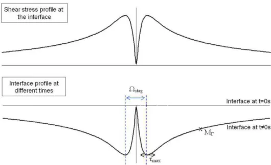
Figure 1.8. Influence of the critical shear stress on the erosion coefficient [Fell et al. 2013]. Figure 2.1. Shear stress profile for a normal flow and theoretical shape of the erosion figure
for a so-called standard erosion law.
Figure 2.2. Illustration of standard erosion figures obtained after Jet Erosion Tests (C. Moras
- geophyConsult).
Figure 2.3. Illustration of the pulsation of an axisymmetric jet in 3-D geometry [Hadziabdic
and Hanjalic 2008].
Figure 2.4. Illustration of the displacement of the jet stagnation point: instantaneous
velocities just above the plane of impingement of the jet at different times [Hadziabdic and Hanjalic 2008].
Figure 2.5. Scheme of the sequential uncoupled erosion model.
Figure 2.6. Subdivisions of regions located close to the wall [Ansys 2009], with u* noted Uτ the friction velocity and y+ =
ρ
y uP *µ
the dimensionless distance from the centre of the first cell to the wall.Figure 2.7. Shape of the mesh before (left) and after (right) a macro-remeshing. Example
taken from the modelling of erosion due to a Poiseuille flow (cf. paragraph 4.1).
Figure 2.8. Shape of the mesh at the beginning (left) and at the end of the erosion process
(right) for the JET performed on soil C (cf. paragraph 3.3).
Figure 2.9. Automation of erosion test models.
Figure 3.1. Geometry and meshing developed for modelling the JETs. Figure 3.2. Refinement of the mesh in the JET configuration.
Figure 3.3. Independence of the results in relation to mesh density, the shear stress on the
water/soil interface before erosion begins, with the k-ω turbulence model.
Figure 3.4. Independence of the results in relation to mesh density, pressure field on the
water/soil interface before erosion begins, with the k-ω turbulence model.
Figure 3.5. Comparison of turbulence models with bibliographical results, velocity field on
the jet centreline.
Figure 3.6. Comparison of turbulence models with bibliographical results: pressure field on
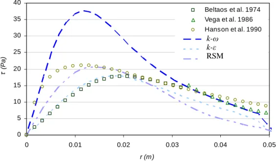
Figure 3.7. Comparison of turbulence models with bibliographical results: shear stress on the
water/soil interface.
Figure 3.8. Velocity field as a function of time in the case of model k-ω above and in the case
of model k-ε below.
Figure 3.9. Evolution of the water/soil interface as a function of time, seen in the upper graph
in the case of model k-ω and in the lower one for the k-ε model.
Figure 3.10. Evolution of scour depth as a function of time. Comparison of numerical results
and [Hanson and Cook 2004] model.
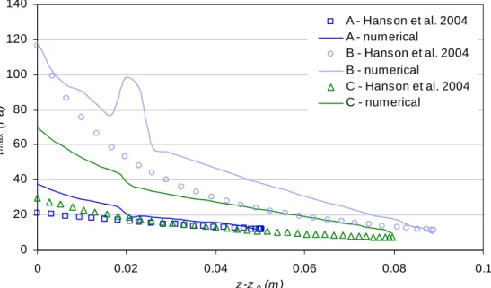
Figure 3.11. Evolution of maximum shear stress as a function of scour depth at different
times for models k-ε and k-ω in comparison to the results of the model of [Hanson and Cook 2004].
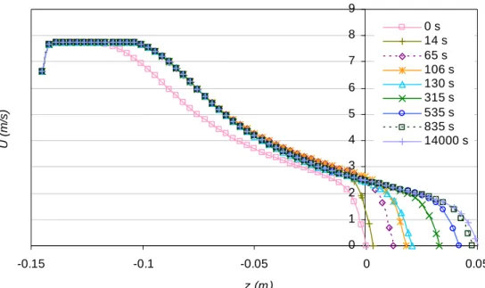
Figure 3.12. Evolution of the velocity field on the jet centreline, model k-ω.
Figure 3.13. Evolution of shear stress on the water/soil interface as a function of time, model
k-ω.
Figure 3.14. Evolution of the pressure field on the water/soil interface as a function of time,
model k-ω.
Figure 3.15. Evolution of the pressure field as a function of time. The results obtained with
the k-ω model shown above and with the k-ε model shown below. Only the values lower than 10% of the full spectrum are shown.
Figure 3.16. Parametric study of the influence of the critical shear stress on the evolution of
scour depth as a function of time for the turbulence model k-ω with kd =10-5 m².s/kg.
Figure 3.17. Parametric study of the influence of critical shear stress on the evolution of scour
depth as a function of time for the turbulence model k-ω, τc=11 Pa or τc=9 Pa.
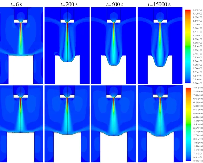
Figure 3.18. Velocity fields relative to the parametric study at times t = 6 s,
t = 200 s, t = 600 s and t = 15000 s, model k-ω.
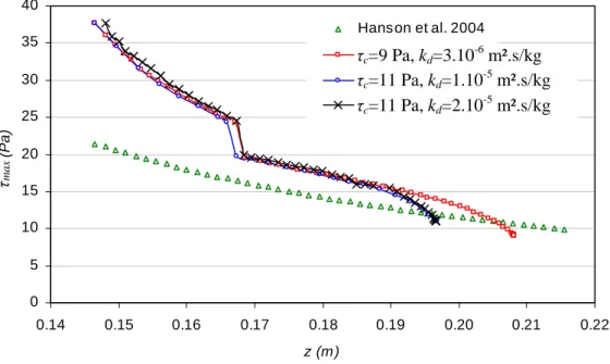
Figure 3.19. Parametric study, evolution of the maximum shear stress as a function of scour
depth at different times.
Figure 3.20. Maximum scour depth as a function of the critical shear stress , model k-ω, kd
=10-5 m².s/kg.
Figure 3.21. Time in which the depth of the cavity has reached half the final depth, plotted as
a function of the erosion kinetics coefficient, τc=11 Pa, model k-ω.
Figure 3.22. Time for which the depth of the cavity has reached half of the final depth plotted
as a function of shear stress, kd =10-5 m².s/kg, model k-ω. Figure 3.23. Granulometric curves of materials A and B.
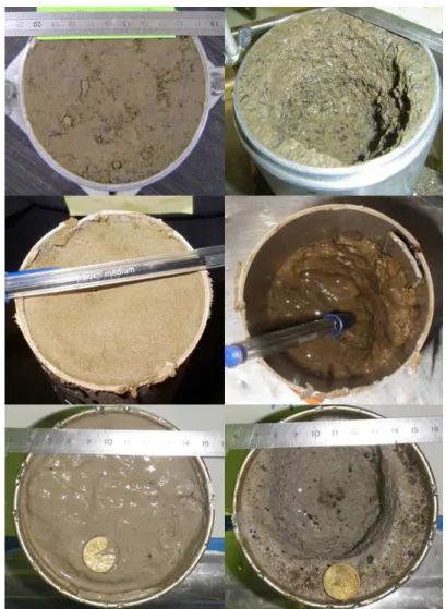
Figure 3.24. Position of soils A, B and C in the classification of [Hanson and Simon 2001]. Figure 3.25. Photographs of soil samples before (left) and after (right) JETs, with from top to
bottom images corresponding to soils A, B and C, respectively.
Figure 3.26. Evolution of the scour depth for tests performed on soils A, B and C, with the
comparison of experimental data and the results of the semi-empirical model.
Figure 3.27. Comparison of numerical results for turbulence models k-ω and k-ε, with the
experimental and semi-empirical results for the test on soil B.
Figure 3.28. Comparison of numerical results for turbulence models k-ω and k-ε, with the
FIGURE CAPTIONS
Figure 3.29. Evolution of the soil/water interface as a function of time with, from top to
bottom, graphs corresponding to the tests performed on soils A, B and C, model k-ω.
Figure 3.30. Shape of the erosion figures obtained numerically, bounded by the mould (black
line) in which the tests were performed on soils A, B and C, model k-ω.
Figure 3.31. Comparison of erosion figures found for the test performed on soil A
numerically and experimentally. Graph bounded by the outline of the mould (black line), model k-ω.
Figure 3.32. Evolution of the shear stress on the soil/water interface as a function of time
with, from top to bottom, graphs corresponding to the tests performed on soils A, B and C, model k-ω.
Figure 3.33. Shear stresses on the water/soil interface at the initial time and critical shear
stresses, for soils A, B and C, model k-ω.
Figure 3.34. Shear stress evolution for the three tests as a function of scour depth, model k-ω. Figure 3.35. Velocity fields and profiles of the soil/water interface as a function of time with,
from top to bottom, results obtained for materials A, B and C, model k-ω.
Figure 4.1. Schematic diagram of modelling the erosion of a channel by laminar flow. Figure 4.2. Velocity profiles at the pipe inlet as a function of time.
Figure 4.3. Velocity fields at different times, with a 1 cm length pipe.
Figure 4.4. Pipe diameter as a function of dimensionless time. Comparison of numerical and
theoretical results.
Figure 4.5. Geometry and shape of the mesh used to model the HETs.
Figure 4.6. Results independency regarding mesh density, the mean velocity field on the axis
of symmetry before erosion begins, for the k-ε turbulence model.
Figure 4.7. Independence of the results from the mesh density, with shear stress on the
water/soil interface before erosion begins, for the k-ε turbulence model.
Figure 4.8. Comparison of the influence of the turbulence model for the velocity field on the
axis of symmetry and for the mean velocity according to axis r.
Figure 4.9. Comparison of the influence of the turbulence model for the pressure inside the
pipe at the erodible walls.
Figure 4.10. Comparison of the influence of the turbulence model for the shear stress on the
water/soil interface.
Figure 4.11. Evolution of the velocity field and the erosion figure as a function of time. Figure 4.12. Evolution of the profile of the water/soil interface as a function of time. Figure 4.13. Evolution of the velocity field on the axis of symmetry as a function of time. Figure 4.14. Evolution of shear stress on the water/soil interface as a function of time. Figure 4.15. Evolution of the pressure field on the water/soil interface as a function of time. Figure 4.16. Evolution of the pressure differential along the useful length. Comparison of the
numerical results with Bonelli’s model [Bonelli et al. 2006].
Figure 4.17. Evolution of the shear stress in x=6 cm, comparison of the numerical results with [Bonelli et al. 2006] model.
Figure 4.18. Evolution of the radius of the pipe diameter. Comparison of the numerical
Figure 4.19. Evolution of the pressure differential between sections A and B. Comparison of the experimental and numerical results and those given by the model of [Bonelli et al. 2006].
Figure 4.20. Evolution of the pressure differential between sections A and B. Comparison of
the results of the parametric study and the experimental data.
Figure 4.21. Evolution of the pipe diameter x=6 cm as a function of time, results of the parametric study.
Figure 4.22. Pipe radius x=6 cm at the end of the erosion process. Comparison of the numerical results given by the model of [Bonelli et al. 2006].
Figure 4.23. Illustration of the erosion kinetics as a function of the erosion coefficient. Comparison of the numerical results and the model of [Bonelli et al. 2006].
Figure 4.24. Illustration of erosion kinetics as a function of critical shear stress, comparison of numerical results and the model of [Bonelli et al. 2006].
Figure 4.25. Granulometric curves of white kaolinite, proclay kaolinite and Hostun sand [Benahmed and Bonelli 2012].
Figure 4.26. Classification of soils tested with the HET in the classification of [Wan and Fell 2004], ○ soil A, ∆ soil D and □ soil E.
Figure 4.27. Evolution of the pressure differential between sections A and B for the tests performed on soils A, D and E, comparison of experimental data with the results of the analytical model.
Figure 4.28. Photographs of soil samples before (left) and after (right) the HET tests, with, from top to bottom images corresponding to the soils A, D and E, respectively (F. Byron, IRSTEA).
Figure 4.29. Comparison of numerical, experimental and semi-empirical results for the HET
on soil A.
Figure 4.30. Comparison of numerical, experimental and semi-empirical results for the HET
on soil D.
Figure 4.31. Comparison of numerical, experimental and semi-empirical results for the HET
on soil E.
Figure 4.32. Evolution of the water/soil interface as a function of time with, from top to bottom, the graphs corresponding to the tests performed on soils D and E.
Figure 4.33. Shape of the scour holes found numerically, comparison of the results obtained
for the tests performed on soils A, D and E.
Figure 4.34. Illustration of typical profiles of scour holes obtained following the HETs (F. Byron, IRSTEA).
Figure 4.35. Evolution of velocity fields and the erosion figure at the end of the erosion process, with, from top to bottom the results obtained for the tests carried out on soils A, D and E.
Figure 4.36. Evolution of shear stress at the water/soil interface as a function of time, with from top to bottom the graphs corresponding to the tests carried out on soils D and E.
Figure 4.37. Shear stresses on the water/soil interface at the initial time and critical shear stresses for soils A, D and E.
Figure 4.38. Evolution of shear stress for the three tests as a function of the radius reached. Values taken in the middle of the erodible pipe.
FIGURE CAPTIONS
Figure 4.39. Evolution of shear stress for the test on soil A as a function of the radius reached. Values taken in x = 6 cm.
Figure 5.1. Erosion coefficient obtained with the JET as a function of the erosion coefficient obtained with the HET.
Figure 5.2. Critical shear stress obtained with the HET as a function of the critical shear stress found with the JET.
Figure 5.3. Ratio of the critical shear stresses obtained for the HET and JET as a function of the water content of the materials tested.
Figure 5.4. Erosion parameters obtained following the test campaign on soil F.
Figure 5.5. Erosion parameters obtained following the tests on the clay/sand mixture.
Figure 5.6. Comparison of results obtained for repeatability tests on soil F, experimentally and using the semi-empirical model of [Hanson and Cook 2004].
Figure 5.7. Critical shear stress as a function of the hydraulic head applied, soil F, z0 =6 cm.
Figure 5.8. Critical shear stress as a function of jet nozzle/soil distance, soil F, ∆ =H 172 cm.
Figure5.9. Erosion rate as a function of shear stress. Comparison of experimental results and the JET and HET interpretation models for soil A.
Figure 5.10. Schematic representation of the flow configuration.
Figure 5.11. Velocity field as a function of the inclined plane, for 90°, 135° and 180°.
Figure 5.12. Vertical velocity profiles above the fixed plane as a function of the inclined plane angle, for 90°, 135° and 180°.
Figure 5.13. Results obtained for the pressure on the horizontal plane as a function of the inclined plane angle.
Figure 5.14. Results obtained for the shear stress on the horizontal plane as a function of the inclined plane angle.
Figure 5.15. Results obtained for the component in x of the pressure gradient on the horizontal plane as a function of the angle of the inclined plane.
Figure 5.16. Results obtained for the component in y of the pressure gradient on the horizontal plane as a function of the inclined plane angle.
Figure 5.17. Results obtained for the dissipation rate of turbulent kinetic energy above the horizontal plane as a function of the inclined plane angle.
Figure 5.18. Results obtained for the turbulent kinetic energy above the horizontal plane as a function of the angle of the inclined plane angle.
Figure 5.19. Results obtained for the flow velocity above the horizontal plane as a function of the angle of the inclined plane angle.
Figure 5.20. Velocity fields above the water/soil interface at t = 0 s obtained for modelling the JET performed on soil A, with the k−ω model.
Figure 5.21. Velocity fields above the water/soil interface obtained at the end of the erosion process for modelling the JET performed on A, with the k−ωmodel.
Figure 5.22. Velocity fields obtained at t = 0 s and at the end of the erosion process (above and below resp.) for the HET model performed on soil A, with the k−ε model.
Figure 5.23. Comparative results of the JET and HET for the shear stress on the water/soil interface.
Figure 5.24. Comparative results of the JET and HET for pressure field on the water/soil interface.
Figure 5.25. Comparative results of the JET and HET for the tangential components of the
pressure gradient on the water/soil interface.
Figure 5.26. The Reynolds number of the turbulent flow as a function of the distance to the
water/soil interface for the JET model, with the k−ωmodel.
Figure 5.27. Reynolds number of the turbulent flow as a function of the axis of symmetry of
the pipe. HET modelling with the k−ε model.
Figure 5.28. Erosion rate as a function of the tangential component of the pressure gradient obtained numerically, for different positions on the water/soil interface and different discretisations of the gradient.
TABLE CAPTIONS
Table 3.1. Meshing parameters examined for the study of the independence of the results
regarding mesh density, with Nnozzle being the number of cells on the nozzle, NCL the number of cells on the water/soil interface and NT the number of cells of the whole calculation domain.
Table 3.2. Comparison of numerical results on a flat plate with results taken from literature. Table 3.3. Identification parameters of soils A, B and C.
Table 3.4. Hydraulic and erosion parameters related to the JETs performed on soils A, B and
C.
Table 3.5. Relative errors on the final scour depth, in comparison to the experimental and
semi-empirical results for the k-ω and k-ε models on soils A, B and C.
Table 4.1. Cell parameters chosen for the study of the results independency regarding mesh
density.
Table 4.2. Identification parameters of soils D and E [Benahmed and Bonelli 2012]. Table 4.3. Hydraulic and erosion parameters of the HETs performed on soils A, D and E. Table 4.4. Relative errors on the final pressure differential between sections A and B,
compared to the experimental and analytical results for soils A, D and E.
Table 5.1. Results obtained with the JET and the HET on the same soils by [Regazzoni et al.
2008], [Wahl et al. 2008] and by IRSTEA and geophyConsult.
Table 5.2. Classification of soils subjected to JETs and HETs in the classification of [Wan
NOMENCLATURE
A normal vector directed to the exterior of the control volume
Aµ constant
c concentration of solid elements in the fluid phase cΓ celerity of the interface
C, C1ε, C2ε and C constants l*
e
C Fell’s erosion coefficient
Cf friction coefficient
Cµ constant or a function of mean deformation 0
d nozzle diameter
d and dɶ grain diameter and dimensionless diameter i
d distance separating the centre of the cell and the interface
D symmetrical part of the mean velocity gradient e state variables or flow variables influencing erosion
E empirical constant
f index attached to magnitudes on surface f fγ, fβ, f and 1 f 2 functions
i
f mean value of the resulting force exerted by the fluid on particles
f and F external volume forces and external surface forces
ij
F force applied on a mesh node
0
Fr Froude number related to grain diameters g acceleration of gravity
1
g and g 2 continuous functions on ℝ+ p
h bed height of particles
HET
I Fell’s erosion rate index (1)
j production term
k turbulent kinetic energy
d
k erosion kinetics coefficient (m².s.kg-1 or cm3.N-1.s-1)
er
k erosion kinetics coefficient (s.m-1)
ij
k spring stiffness between nodes i and j 0
k meand turbulent kinetic energy between the surface of the material and the free surface
kP turbulent kinetic energy of the fluid at node P
soil
k gauge of hydraulic permeability of soil near the interface
er
kɶ dimensionless erosion number K intrinsic permeability fs K penalisation coefficient r K height of asperities s
K penalisation parameter of fluid velocity field in the soil
s
K+ dimensionless height of asperities
l length of potential core of immersed circular jet
w
ℓ characteristic dimension of the fluid domain Γ
ℓ characteristic dimension of the zone close to the interface
lµ characteristic length of the two-layer model resolving the boundary layer
u
L useful length
mɺ flux of eroded mass
MΓ point of the water/soil interface
n number of particles per unit of volume
n
unit normal at Γ oriented towards the soili
n number of neighbouring nodes connected to i
m
n mass fraction
N number of faces composing the control volume
Nnozzle, NCL and NT number of mesh cells on the nozzle, interface and total number of cells
p pressure
p' pressure fluctuations
i
p pressure at the scale of the pore
w
p pressure in the fluid phase
( )
P r distribution of pressure at the water/soil interface
k
P ( Pε and Pω resp.) source term of production of k (
ε
and ω resp. )max
P value of peak pressure on the surface of impact at the jet centreline
R
P source term of production of the RSM model
i
q filtration velocity
s
q eroded flow rate of sediment per unit of length
r distance to the axis of symmetry (jet centreline or pipe symmetry axis) 0
r averaged intensity of turbulence between the surface of the soil and the freesurface
rmax radius of the soil sample for the JET
( )
R t and R tɶ
( )
radius of the erodible pipe and dimensionless radius R tensor of turbulent stresses0
R and R∞ initial radii of the pipe and radius at time t∞
Re, Rep and Rey Reynolds number of the flow, particle and turbulence 0
Re Reynolds number of the flow at the nozzle outlet orifice
A
S and S1 surface of sections A and 1
amont
S , Saval surfaces of sections located upstream and downstream of a geometrical singularity
Sφ source term of
φ
w by unit of volumet, tɶ andter times, dimensionless and characteristic erosion times
1/ 2
t time in which the erosion depth reaches half of z∞−z0 T Cauchy stress tensor
u axial velocity of flow
u axial velocity vector of flow
u′ fluctuations of velocity in relation to the mean velocity
*
u , U τ velocity of friction at the water/soil interface
axis
NOMENCLATURE
b
u axial velocities of the fluid at the interface
w i
u mean local velocities of fluid
p i
u mean local velocities of particles
in
u input velocity of flow
moy
u mean velocity of flow between two erodible walls
s
u and uw values of u on Γ soil side and flow side 0
U jet velocity at the nozzle
i
U mean velocity of two-phase mixture
m
U mean flow velocity between the surface of the material and the free surface
UP principle component of the fluid velocity at node P located near wall v radial velocity of the flow
b
v radial velocities of the fluid at the interface
vΓ velocity of the interface v' fluctuations of velocities
V control volume
w
V gauge of the flow velocity
er
V gauge of the erosion velocity
er
Vɶ erosion kinetics
w ' fluctuations of velocities
W mechanical work of flow between the inlet and outlet of the system
x abscissa in an orthonormed reference point
1
x abscissa of section 1 X interface node
yP distance separating node P from the wall
*
y andy+ dimensionless distance from the centre of the first cell to the wall
k
Y (Yε and Yω resp.) source term of the dissipation of k (
ε
and ω resp.)R
Y source term of the dissipation of the RSM model
ref
Yɶ concentration in solid particles
z distance separating the height of the jet outlet and the interface at the jet centreline
1/ 2
z ordinate of the interface characterised by zɶ1/2 = zɶ0 +
(
zɶ∞ −zɶ0)
2 0z distance separating the height of the jet outlet and the interface at t=0 s
z∞ distance z at the end of the erosion process, at time t=+∞
zɶ, zɶ0, zɶ and ∞ zɶ1/ 2 dimensionless distances z , z0, z∞ and z1/ 2
Greek letters
α coefficient as a function of the Reynolds number
0
α , α , τ
β
i andβ
∞* constantsΓ water/soil interface
γ critical non intrinsic stress at the soil
∆B corrective term of roughness
h
∆ head loss
H
∆ applied hydraulic head
0 p
P ∆ pressure differential at t 0 P ∆ pressure differential at t=0 s t
∆ erosion time step
i x
∆ and ∆xj displacements of node i and its neighbour j
ε rate of viscous dissipation of turbulent kinetic energy
P
ε rate of viscous dissipation of turbulent kinetic energy at node P
w
ε
void fractionθ slope of plane in relation to the horizontal wall
c
θ critical Shields number
κ Von Karman constant
λ diffusion coefficient
rb
λ Borda-Carnot discharge coefficient for a sudden widening
p
λ discharge coefficient
φ
λ diffusion coefficient of φw by unit of volume
t
µ turbulent viscosity
w
µ dynamic viscosity of the fluid
w
ν kinematic viscosity of the fluid
ξ non-intrinsic erosion coefficient on the soil
ρp density of particles
s
ρ dry density of the soil
w
ρ density of the fluid
τ shear stress, norm of the tangential component of the stress tensor on Γ
*
τ mean shear stress that takes into account the fluctuations of instantaneous stress values
τc and τɶ c critical shear stress and dimensionless critical stress
max
τ maximum shear stress
w
τ shear stresses of the fluid phase
τp shear stresses of the particle phase
τΓ gauge of shear stress on the interface
|τ | and |b τ | viscous shear stress exerted on the soil and on the fluid g
f ij
σ effective stress tensors linked to the fluid phase
p ij
σ effective stress tensors linked to the particle phase
φ porosity
p
φ volume fraction of particles
w
φ flow variable
f
φ flow variable calculated at one surface
f
φ weighted average of values of φf on all the nodes composing the surface
ϕ Level-Set function
χ characteristic parameter of the sediment bed
ψ one variable or the whole variable driving erosion
ω specific dissipation rate
Ω rotation of mean velocity gradient
w
Ω and Ωs fluid and solid domains
stag
NOMENCLATURE
Acronyms
ARS Agricultural Research Service CFD Computational Fluid Dynamics DNS Direct Numerical Simulation EFA Erosion Function Apparatus JET Jet Erosion Test
HET Hole Erosion Test LES Large-Eddy Simulations VOF Volume of Fuid
RANS Reynolds Average Navier Stokes RSM Reynolds Stress Model
SD Strongly Deflected Regime
SIMPLE Semi-Implicit Method for Pressure-Linked Equations WD Weakly Deflected Regime
INTRODUCTION
Erosion mechanisms are the main causes for breaches in embankment dikes and dams. That is why it is vital to be able to quantify the resistance to erosion of soils making up embankment structures and their foundations, to prevent any risk of disaster and, if necessary, strengthen them. To do this different systems have been developed: notably jet erosion testers such as the Jet Erosion Test (JET) and piping erosion tests such as the Hole Erosion Test (HET). These two tests were developed by [Hanson and Cook 2004, Lefebvre et al. 1985] respectively. They are designed to grade the sensitivity of soils to erosion in the laboratory or in-situ by performing standardised tests. The HET was developed in Australia at the University of Sydney by the teams of R. Fell, and that of the JET in the United States at the Agricultural Research Service (ARS) by the teams of G. Hanson. A priori, these tests allow to answer the following three questions about the different materials tested: When is the erosion triggered? What is the speed of degradation by erosion? When does the erosion stop? The determination of erosion parameters: the erosion threshold or critical shear stress and the erosion kinetics coefficient, permit answering these questions. Nevertheless, the values of the erosion parameters obtained following these two tests present major differences, as highlighted by [Regazzoni et al. 2008, Wahl et al. 2008]. These differences persist in spite of the improvement of the HET interpretation model by [Bonelli et al. 2006] and several modifications made by [Pinettes et al. 2011] to the JET interpretation model.
The equations related to the HET interpretation model developed by [Bonelli et al. 2006] are mechanically proven. On the contrary, the basic equations of the JET model remain empirical. That is why the aim of this thesis is to determine the pertinence of the JET interpretation model. To do this, a numerical model of the test, based on the erosion phenomena that characterise it, was necessary. With the only information being the boundary conditions imposed on the flow during the test and the erosion parameters obtained with the JET interpretation model, is it possible to numerically simulate the evolution of the soil/water interface observed experimentally? To our knowledge the literature does not include any numerical model of the erosion of a cohesive soil by a turbulent flow in a configuration such as that used for erosion tests. The development of such an erosion model brings into play major numerical challenges.
The present thesis focuses on the numerical modelling of the erosion of a cohesive soil by a turbulent flow with, initially, its application to the erosion by a jet flow with a stagnation point. The objective of this work is to better understand the phenomena involved during erosion under a normal turbulent flow, and to conclude on the pertinence of the JET interpretation model used at present.
The first difficulty that becomes apparent in this context is taking into account the two-phase nature of the flow. The thesis by [Brivois 2005] permits defining the foundations of two-phase modelling: for situations encountered in practice, flow velocity is several orders of magnitude greater than erosion velocity. Consequently, the quantity of mass eroded is small enough to
permit considering a diluted flow and single-phase modelling for the turbulent flow [Bonelli
et al. 2012].
The second difficulty is the representation of the mobile interface and the precise calculation of the mechanical quantities on it. The solid/fluid interface is considered as singular and not as a third fluidised solid phase. In the case of the numerical simulation of flows in the presence of interfaces, two main approaches can be distinguished: capturing or monitoring the interface. The first, called the Eulerian approach, consists in defining the media (water-soil) in a given domain (fixed mesh) and determining its evolution. The second is known as the Eulerian-Lagrangian approach, which consists in displacing the frontier over time (mobile meshing). [Lachouette et al. 2008] developed an original 2D/3D laminar incompressible viscous flow with erosion for a flow diluted on obstacles. In this framework, the interface is represented by the fictitious domains method and its evolution is described by the Level-Set method within a fixed Cartesian grid. The advantage of the Eulerian approach is that it does not require complex meshing. Fine modelling of the quantities at the interface is nonetheless problematic using this approach. This is not the case with the mixed approach which nonetheless introduces major remeshing problems. The numerical deadlocks inherent to the simulation of erosion processes lead to considerable modelling issues.
The third difficulty concerns the erosion law of a fine or granular soil with or without cohesion. Erosion is defined by a flow of mass crossing a solid/fluid interface assumed to be singular and mobile. The erosion law can be assimilated with a constitutive law linking the celerity of the interface and the mechanical magnitude(s) representing the driving force. The system of equations can be simplified by evaluating the orders of magnitude of the phenomena [Bonelli et al. 2012]. The complexity of the phenomena generated by the stagnation point of the turbulent jet flow must also be taken into account in the erosion law.
Once the numerical model has been developed, the results obtained will be compared to experimental results and to the results of the semi-empirical model of [Hanson and Cook 2004]. Then, an additional validation of the modelling method will be performed in the piping erosion configuration. The results obtained for modelling the HET tests will be compared to the experimental results and to the results of the analytical model of [Bonelli et al. 2006]. The results obtained will be used to perform an in-depth study of the erosion law and the physical signification of the erosion parameters.
This thesis is divided into five chapters. The first chapter provides a description of the state-of-the-art underlying this study. The first part concerns the elements linked to erosion in hydraulic works and its experimental and analytical determination. The second concerns the numerical modelling of erosion. The context related to erosion in hydraulic works is given first after which the consequences of erosion at the scale of the structure are described. Then, the methods used to determine the erodability of soils and the associated erosion meters are presented. Next, we focus on the two most commonly used erosion meters to determine the resistance of soils to erosion: the JET and the HET. This is followed by a discussion on the different empirical models used to determine erosion rates and threshold stresses.
INTRODUCTION
In the second part, the context related to the numerical modelling of erosion is described. The most pertinent numerical modelling methods are presented, with, first of all, approaches that consider the water/soil interface as a fluidised solid interface and, secondly, the approach that considers a singular interface.
We describe the modelling method we propose in the second chapter. We first establish the hypotheses on which the model is based after which we set out the equations governing the behaviour of the fluid followed by those governing erosion. This is followed by a part on numerical modelling that will permit describing in particular the discretisation and remeshing methods used.
In the third chapter, the modelling method is applied to normal flows and more specifically to the configuration of JET tests. Initially, we underline the development and validation of the numerical model. Then, the modelling results of three JETs will be analysed, in comparison to experimental data, making it possible to provide important information on the pertinence of the JET interpretation model.
In the fourth chapter, the modelling method is then applied to piping erosion. The method is first validated on the erosion of a channel by a Poiseuille flow. This is followed by numerical modelling of the HET tests. We first develop and validate the numerical modelling in this configuration. Then we study the results of modelling the HETs in comparison to experimental data. Additional elements for validating the modelling method are deduced from these results.
The fifth chapter presents an in-depth study of the erosion law and the differences between JET and HET. The first part of this chapter concerns the differences between the erosion parameters found after these two tests and their pertinence. The second part sets out a study of the variables susceptible to drive and influence erosion. We also focus on the signification of the erosion parameters found after the JET and HET tests. Lastly, consideration is given to paths for developing the erosion law.
Chapter 1.
State of the art
The objective of this chapter is to present how this thesis permits answering an industrial need and a scientific problem in an original way accessible in terms of calculation time. The state of the art described first concerns erosion in hydraulic structures. This part serves to explain why determining the resistance of soils to erosion remains a challenge, the ways in which it can be determined and the physical phenomena that, a priori, govern soil erosion. It also explains why it is necessary to develop a numerical modelling method to simulate the erosion of cohesive soils by turbulent flows. The second part of this chapter presents the state of the art related to the numerical modelling of erosion. The most finalised modelling methods are presented. It also permits determining why existing methods cannot solve the problematic we put forward.
1.1.
Erosion in hydraulic structures
1.1.1. Context1.1.1.1. Erosion at the scale of the structure
Erosion, whether internal or surface, is one of the main mechanisms leading to the breaching of embankment dikes and dams. [Fry 2012] performed a complete evaluation of internal erosion in dams and dikes and the main lines are summarised in this paragraph. France has more than 700 large dams, about ten thousand small dams (height lower than 15 m), and nearly 8,000 km of navigation channel dikes and 10,000 km of flood protection dikes. Most of these hydraulic structures were built more than half a century ago using natural materials found on the construction site. Since these structures were built with natural materials without binders, the term embankment structure is used. In 1995, the International Commission of Large Dams drew up a list of the large dams in the world (excluding China). It identified three times more dams built of loose materials than of concrete or masonry. Nearly fifteen times more breaches have been recorded for embankment dams than for other types. Embankment dams are therefore vulnerable structures whose breaching modes can be classed into two
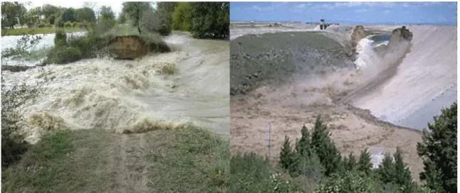
categories. The first is subsidence or general instability while the second is erosion, which is defined by local washing away of grains, and internal and localised instability. [Foster et al. 2000] calculated the world breaching statistics for large dams and established that 94% of breaches are due to erosion. Whether internal or external, erosion is responsible for one breach of a hydraulic structure a year in France on average. Most of these breaches take place during heavy floods, such as the breach caused by the flood of the River Gard in September 2002 (5 deaths, damage amounting to €1.2 billion) and those caused by the flood of the River Rhone in December 2003 (damage amounting to €845 million). Figure 1.1 illustrates these dam and dike breaching phenomena.
Figure 1.1. Breach caused by flooding of the Virdourle river in 2002 (left) and breach of the
Teton Dam, 1976 (right).
Internal erosion is caused by an underground flow and external erosion is caused by a flow on the surface of the structure. Internal erosion can be generated by four mechanisms: piping erosion, regressive erosion, contact erosion and suffusion. Various mechanisms trigger internal erosion: cracks of geological origin, rotting tree roots, contact between the soil and a discharge conduit, etc.
Piping erosion such as that defined by [Bonelli et al. 2012] is characterised by a flow of water that washes away particles along a preferential path. Thus a hydraulic pipe forms and widens as erosion progresses. This erosion mechanism may rapidly lead to a breach in the hydraulic structure. Regressive erosion is characterised by erosion of the soil from downstream to upstream, in the opposite direction to the flow. The soil particles are first washed downstream where the flow erodes the surface of the soil at its outlet, then the erosion propagates from downstream to upstream of the flow. The causes of regressive erosion are mainly an increase of the hydraulic gradient during floods or the alternation of layers of sandy, silty and clayey materials [Beek et al. 2013, Fell and Fry 2007]. Contact erosion [Beguin et al. 2012, Philippe
et al. 2013] is the washing away of particles in a flow that takes place at the interface between
two layers of different soils inside a hydraulic structure. It often occurs immediately the structure is filled with water. As for suffusion, it is characterised by the washing away of fine particles located in the interstitial voids of a matrix of coarser material [Marot et al. 2012].
CHAPTER 1. STATE OF THE ART
1.1.1.2. Estimation of soil erodibility
The objective of the decree issued on 11 December 2007 was to improve the safety of hydraulic structures in France. In particular it gives priority to revising the procedures for monitoring and studying the hazards for certain structures. So that the managers of hydraulic structures can assess their reliability, it is necessary to quantify the erosion resistance of the soils that compose them. A certain number of mechanical tests on soils have been developed to estimate their erodibility.
Mention can first be made of erosion tests in flumes, used by [Gibbs 1962, Partheniades 1965] among others. The soil samples are placed in a flume on all or part of its surface. The mass eroded is either determined by weighing the samples (Hydraulic Flume Test) or by measuring the particles in the flow at the flume outlet. The Erosion Function Apparatus (EFA) developed by [Briaud 2001] also consists in passing a flow at a controlled velocity over the surface of a soil sample. The erosion rate of the soil is controlled by a piston system located under the sample. These tests aim to be representative of external erosion such as the erosion of river beds and around bridge piers. The Rotating Cylinder Test of [Moore and Mash 1962] is a cylindrical device in which a fixed cylinder of soil is placed. Water is injected between these two parts of the device and it is brought into movement. The Drill Hole Test of [Lefebvre et
al. 1985] is inspired by the Rotating Cylinder Test. An initial cylindrical hole of about 6 mm
in diameter is made in a soil sample in which a flow under pressure is made to circulate. This test gave rise to the Hole Erosion Test (HET) of [Wan and Fell 2004] with a controlled flow rate. The quantity of mass eroded is calculated on the basis of measurements taken upstream and downstream of the soil sample. The Hole Erosion Test is representative of internal piping erosion. Jet erosion meters have also been the subject of many studies. Their advantage is that they can be used in-situ. The Mobile Jet erodibility meter [Hénensal 1983] consists of the impact of seven mobile jets on the interface of the material. The rate of erosion is calculated from the measurement of the quantity of soil in the flow leaving the device. This device is designed to simulate the impact of rain droplets and runoff. The Jet Erosion Test (JET) developed by [Hanson and Cook 2004] is an erosion test during which a jet with a controlled flow rate impinges on the surface of a soil sample. The entire system is immerged in a tank adapted for the laboratory and the field. Erodibility is calculated by measuring the depth of the cavity formed as a function of the time the jet impinges on the material. This test is representative of external erosion by spillover downstream of the structure.
1.1.1.3. Erosion parameters
The Hole Erosion Test and Jet Erosion Test are adapted to characterising the resistance of soils to erosion for embankment dams and dikes. The interpretation models of these two tests are based on an erosion law that considers erodibility as function of shear stress exerted by the soil on the soil sample. This law is governed by two parameters characteristic of soil resistance to erosion. It entails an erosion threshold from which the hydraulic power supplied is sufficient to generate erosion and an erosion coefficient. The erosion threshold is a critical
shear stress that can range from 0 to103 Pa. The erosion coefficient also varies by several orders of magnitude, from 10-2 to 10-6 s/m. It is a coefficient of proportionality between the mass flux of the eroded soil and the shear stress exerted by the fluid on the soil (minus the critical shear stress). It can be considered as the ratio between a characteristic dimension and the surface viscosity of the eroded soil [Bonelli et al. 2012]. The erosion threshold and the erosion coefficient are used to classify the soils on a scale of erodibility. They also provide the bases of models to determine the time to breaching of structures. These parameters are a
priori intrinsic to the soil and therefore should be the same whatever the test considered.
However, [Regazzoni et al. 2008, Wahl et al. 2008] showed that for the same soil, the erosion parameters obtained with the JET and HET can differ by one or two orders of magnitude.
1.1.2. HET and JET erosion tests
1.1.2.1. The Hole Erosion Test
The Hole Erosion Test is a laboratory test device used to study concentrated leak erosion, also called piping flow erosion. The erosion test apparatus was introduced by [Lefebvre et al. 1985] and developed by [Wan et al. 2002].
The experimental device used by IRSTEA operates with a flow rate maintained constant during the test. An intact or disturbed soil sample is placed in the test device. An initial hole of a few millimetres in diameter is created in the sample. The pierced sample is subjected to flow under pressure. The soil sample will be eroded if the stress exerted by the flow is sufficiently strong the erosion causes the diameter of the pipe to increase. The pressure gradient is measured throughout the test. The measurements permit determining the evolution of the diameter of the initial hole and the shear stress exerted by the fluid on the soil interface [Bonelli et al. 2006]. Continuous turbidity measurements are also performed during the test. Figure 1.2 shows how the Hole Erosion Test works and the notations used. For the sake of clarity, the scale is not quite the same as that used in reality, given the classical dimensions of the soil sample: from 12 to 15 cm in length and 8 cm in diameter. The initial hole usually has a diameter of 6 mm. The photograph of the experimental device adapted by IRSTEA is presented in Figure 1.3.
Figure 1.2. Simplified schematic diagram of the Hole Erosion Test.
L
r
x
( )
R t Water inlet Axis of symmetry Soil sample Pressure sensors Water outlet Interface at t = 0 s Interface at t > 0 sCHAPTER 1. STATE OF THE ART
The first HET interpretation model was developed by [Wan and Fell 2004]. This model is used to determine an erodibility index and an erosion threshold, the critical shear stress. It relies on the linear approximation of the curve of the mass eroded as a function of the shear stress exerted by the fluid on the soil/water interface. The determination of a friction coefficient is then needed. The shear stress and the friction coefficient are estimated using semi-emprical formulas.
A second HET interpretation model was developed by [Bonelli et al. 2006]. This model is mechanically based on incompressible Navier-Stokes equations in cylindrical geometry. The most commonly used erosion law in the domain of soil mechanics is implemented (cf. paragraph 1.1.3):
(
)
if 0 else er c c k mɺ = τ−τ τ>τ (1.1)with mɺ flux of eroded mass, τ shear stress exerted by the flow on the soil, τc critical shear
stress and ker erosion coefficient expressed in (s.m-1). The erosion coefficient can also be expressed in (m².s.kg-1 or in cm3.N-1.s-1). It is then noted kd and is such that ker =
ρ
skd withs
ρ
being the mean dry density of the soil.u and v are the axial and radial velocities, p is the pressure in the flow, and
ρ
w is the density of the fluid. The equations of mass conservation and quantity of movement give, respectively [Bonelli et al. 2006]:( )
1 0 rv u r r x ∂ + ∂ = ∂ ∂ (1.2)( )
2( )
1 1 w p u rvu u r t r r x r r x ∂ ∂ ∂ ∂ ∂ + + = − − ∂ ∂ ∂ ∂ ∂ ρ τ (1.3) 0 p r ∂ = ∂ (1.4)The boundary conditions of the flow are the following jump equations defined by [Bonelli et
al. 2006], with Γ water/soil interface:
1 1 = − b s w v m
ρ
ρ
ɺ , Γ = s m v ρ ɺ (1.5) 0 b u = , τb = τg (1.6)with Γ being the water/soil interface, u and b v are the axial and radial velocities of the fluid b
at the interface, vΓ the velocity of the interface, τb and τg the shear stresses exerted on the soil and on the fluid, respectively.
Figure 1.3. Photograph of the experimental Hole Erosion Test device.
Figure 1.4. Grouping of HET test results for a flow rate imposed on the master curve defined by equation (1.7) of [Bonelli et al. 2012].
The analytical model of [Bonelli et al. 2006] gives the evolution of different variables in a pipe subjected to erosion. For pipe erosion at a constant flow rate, the governing equations are the following:
1/4 1/4 5/4
(τc ) (τc ) τc
f ɶ Rɶ = f ɶ + ɶ tɶ with ( ) 1
(
arctan arctanh)
2 f x = x+ x −x (1.7) er t t t = ɶ , 0 τ τ τ c c = ɶ ,
( )
( )
0 R t R t R = ɶ (1.8) 0 2 er d L t k P = ∆ , τ 2 R P L ∆ = , R tɶ( )
= ∆ P tɶ( )
−1/5 (1.9) with τ and τ0 ɶc being the initial and dimensionless critical shear stress, ∆P and ∆P0 the pressure differential between the inlet and the outlet of the pipe at t and t=0 s, R t( )
, R0 andCHAPTER 1. STATE OF THE ART
( )
R tɶ the radius of the erodible pipe of length L at time t, initially and with a dimensionless radius; t , ter and tɶ time, the characteristic time and the dimensionless time.
The validation of this simplified model was performed for different HETs, as can be seen in Figure 1.4.
1.1.2.2. The Jet Erosion Test
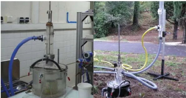
The Jet Erosion Test is an erosion measurement device characterised by an immersed water jet impinging on the soil surface. The test device is used to study the resistance of soils to erosion in the laboratory and in-situ. Many studies have used jets to quantify the characteristic parameters of a soil subject to erosion in the laboratory [Hanson and Robinson 1993, Hollick 1976, Mazurek et al. 2001, Moore and Mash 1962] and in-situ[Allen et al. 1997, Hanson 1991]. The experimental test device developed by [Hanson and Cook 2004] and the associated methodology initiated a large number of experimental studies to determine erodibility, including [Langendoen et al. 2000, Pinettes et al. 2011, Regazzoni et al. 2008, Robinson et al. 2000, Simon and Thomas 2002].
The soil sample can be part of the hydraulic structure in-situ, or intact or disturbed in the laboratory. It is subjected to flow under pressure. The water is set in circulation with a constant pressure drop. The flow is perpendicular to the impinged region. The soil sample will be eroded if the shear stress exerted by the flow is sufficiently strong. Measurements of scouring depth are performed throughout the test. They allow determining the characteristic parameters of the soil subjected to erosion: the erosion coefficient and the critical shear stress. Figure 1.5 shows how the Jet Erosion Test works and the notations used. Figure 1.6 presents two photographs of the experimental test device in the laboratory and in-situ. This apparatus is that used at present by geophyConsult [Pinettes et al. 2011], and it was also used for the study [Regazzoni et al. 2008].
The interpretation model of the Jet Erosion Test was developed by [Hanson and Cook 2004]. It is based on the analytical approach of [Stein and Nett 1997] developed in the case of plane jets. The governing equations of the model of [Hanson and Cook 2004], excluding the erosion law (1.1) are the following:
0 2 U = g H∆ (1.10)
( )
0 l U z U z = (1.11) 0 6.2 l = ×d (1.12)( )
2 f w C U z τ = ρ (1.13)with g being gravity, U the velocity of the jet at the nozzle, 0 ∆H the hydraulic head applied, l the potential core length, z the distance separating the height of the jet outlet and