HAL Id: hal-03151539
https://hal.archives-ouvertes.fr/hal-03151539
Submitted on 24 Feb 2021
HAL is a multi-disciplinary open access
archive for the deposit and dissemination of
sci-entific research documents, whether they are
pub-lished or not. The documents may come from
teaching and research institutions in France or
abroad, or from public or private research centers.
L’archive ouverte pluridisciplinaire HAL, est
destinée au dépôt et à la diffusion de documents
scientifiques de niveau recherche, publiés ou non,
émanant des établissements d’enseignement et de
recherche français ou étrangers, des laboratoires
publics ou privés.
PSM-nets: Compressing Neural Networks with Product
of Sparse Matrices
Luc Giffon, Stéphane Ayache, Hachem Kadri, Thierry Artières, Ronan Sicre
To cite this version:
Luc Giffon, Stéphane Ayache, Hachem Kadri, Thierry Artières, Ronan Sicre. PSM-nets: Compressing
Neural Networks with Product of Sparse Matrices. IJCNN, Jul 2021, Virtual Event, United States.
�hal-03151539�
PSM-nets: Compressing Neural Networks with
Product of Sparse Matrices
Luc Giffon
∗, Stéphane Ayache
∗, Hachem Kadri
∗, Thierry Artières
∗†and Ronan Sicre
∗†∗Aix Marseille Université, Université de Toulon, CNRS, LIS, Marseille, France †École Centrale Marseille, Marseille, France
Abstract—Over-parameterization of neural networks is a well known issue that comes along with their great performance. Among the many approaches proposed to tackle this problem, low-rank tensor decompositions are largely investigated to com-press deep neural networks. Such techniques rely on a low-rank assumption of the layer weight tensors that does not always hold in practice. Following this observation, this paper studies sparsity inducing techniques to build new sparse matrix product layers for high-rate neural networks compression. Specifically, we explore recent advances in sparse optimization to replace each layer’s weight matrix, either convolutional or fully connected, by a product of sparse matrices. Our experiments validate that our approach provides a better compression-accuracy trade-off than most popular low-rank-based compression techniques.
Index Terms—neural networks, compression, sparsity
I. INTRODUCTION
The success of neural networks in the processing of struc-tured data is in part due to their over-parametrization, which plays a key role in their ability to learn rich features from data [1]. Unfortunately, this also makes most state-of-the-art models too large to store and impossible to operate on devices with limited resources or that cannot integrate a GPU [2]. This problem has led to a popular line of research: “neural networks compression”, which aims at building models with few parameters while preserving their accuracy.
Many popular matrix and tensor decomposition methods including Singular Value Decomposition (SVD), CANDE-COMP/PARAFAC (CP) and Tucker are used to address the problem of model compression by a low-rank approximation of the neural network’s weights after learning. Few of these methods are proposed for dense layers first [3] and extended to convolutional layers [4]–[6]. But these methods rely on low rank assumption that may be too strong. More recently the Tensor-Train (TT) decomposition is proposed to compress both dense and convolutional layers [7] and achieved extreme compression rates, yet at the price of impractical downsides that we detail in Section II-C.
Other compression methods include unstructured pruning techniques that we review in more details in Section II-C and structured pruning techniques that reduce the inner hidden di-mensions of the network by completely removing neurons [8]. According to the recent paper [9] however, these techniques are more akin to Neural Architecture Search than network compression. Finally, quantization-based compression maps the columns of the weight matrices in the network to a subset
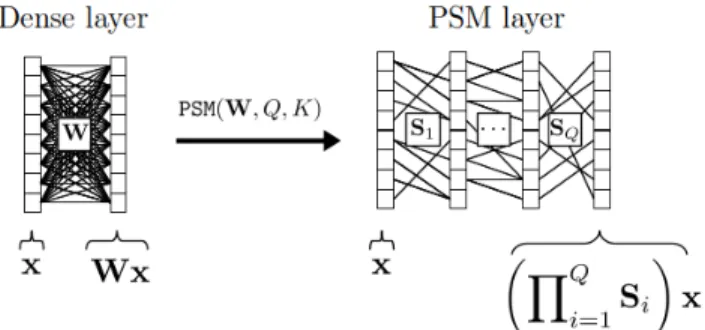
Fig. 1: Diagram of the PSM compression of a dense layer.
of reference columns with lower memory footprint [10]. These two latter families of compression techniques are out of the scope of this paper as they are not necessarily incompatible with sparsity and low-rank based compression techniques, which are our focus of interest here.
We are specifically interested in high-rate compression of a neural network by efficiently factorizing its layers’ weight matrices, as products of sparse factors. There are two main reasons for exploring this line of research.
First, while the most well known approaches for layer decomposition make low-rank assumption on the layer weight tensors, this assumption may not hold in practice. As we show experimentally, the Tucker and SVD based techniques are indeed unable to reach high compression rates for standard architectures including both convolutional and fully connected layers, such as VGG19 or ResNet50.
Second, products of sparse factors are known to enable fast computation without any low rank assumption. Fast operators like the Hadamard and the Fourier transforms are well known low complexity linear transforms. Recall that a standard linear operator (i.e. a matrix) from RD to RD has time and space
complexities of O(D2) but the Hadamard and the Fourier
transforms can be expressed in the form of a product of log D sparse matrices, each having O(D) non-zero values [11], [12]. These linear operators, called fast-operators, thus have time and space complexities lowered to O(D log D).
Interestingly while every factor in a product may include only few non-null parameters, their product can still represent high-rank matrices, up to a full rank matrix. A product of such sparse matrices with a given sparsity budget, i.e.number of non zero values, is strictly more expressive than a single
matrix with the same budget [11]. This interesting feature inspired several works based on the idea that sparse matrix product representations of existing fast-transforms could be learned [11]. [12], [13] aim at computing such sparse product approximations of any matrix in order to accelerate learning and inference. Even though these methods are originally designed to recover the log D factors corresponding to a fast-transform, they can be used to find an approximate factoriza-tion with Q < log D sparse matrices, hence enabling even more computation speed-up.
Our contributions are as follows. We introduce a general two step framework for neural network compression. First, we rely on a procedure that approximates every layer with a PSM-layer by factorizing the PSM-layers’ weights into a product of sparse factors (see Figure 1 for an example on a dense layer). Second the resulting net, built by cascading all these PSM-layers, is refined with standard gradient descent. We provide an extensive evaluation of the recently proposed palm4MSA algorithm [12] for the approximation of an orginal layer (dense or convolutional) with a PSM-layer. We investigate the behaviour of our approach and the impact of the PSM-layer learning procedure on the overall result, with respect to accuracy and compression rate. We compare our approach and its variants with state of the art compression methods on well known deep architectures learned on standard benchmarks. Our experimental results show that layers’ weights may be factorized into very few sparse matrices while preserving accuracy, hence achieving very high compression rates.
II. LEARNING SPARSE MATRIX PRODUCTS FOR NETWORK COMPRESSION
This section describes the proposed method for compressing all layers’ weights of a pretrained network. First, the linear transform operations involved in fully-connected and convo-lutional layers is detailed. We also show how propagation in both types of layer is cast as a matrix product. Then, the NN compression framework is described. Finally, a few known neural network compression techniques are reviewed; some of them are shown to be particular cases of our framework. A. Weight matrix as a product of sparse matrices
Fully-connected and convolutional layers are based on the computation of linear operations. In a fully-connected layer, the output z ∈ RD0 is simply given by z = a(Wx) where a
is a non-linear activation function. W ∈ RD0×D is the weight
matrix of the layer and x ∈ RDis the output of the preceding
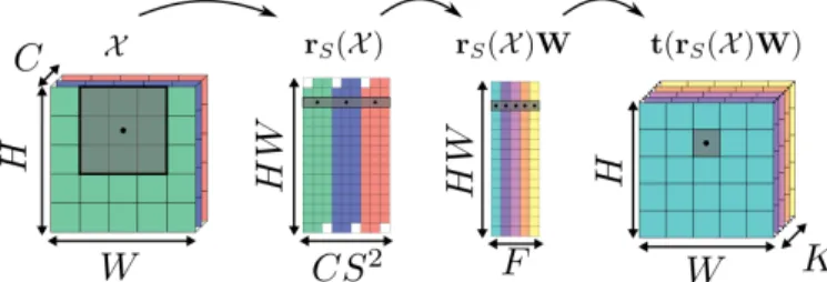
layer. The linear operation in a convolutional layer may be represented as a doubly-block Toeplitz matrix [14]. Another way to perform the operation is to employ reshaping operators to represent the linear operator as a dense matrix applied to all the patches extracted from the input [15]. Thus, we can cast the compression of dense and convolutional layers as the same problem of approximating a matrix with a product of sparse matrices. Note that we later rely on this feature in next section. More formally, let rS : RH×W ×C 7→ RHW ×CS
2
be the reshape operation that creates the matrix of all vectorized
patches of size (height and width) S2on an input image with
C channels. The matrix of F filters W ∈ RCS2×F can then be
applied to these patches (transformed with rS) to produce the
output of the convolutional layer in a matrix shape. Finally, a second reshape operator t : RHW ×F 7→ RH×W ×F is
applied on this feature map matrix to recover the tensor output of the convolutional layer Z ∈ RH×W ×F. Altogether, the convolution operation can be written as Z = a(t(rS(X )W))
where a is some non-linear activation function and X is the output 3-D tensor of the preceding layer. We preserve simplicity in notation here, assuming without loss of generality that the stride used by rS is equal to 1 and that the input
tensor is padded with bS2c zeros vertically and horizontally. The whole process is depicted in Figure 2.
Fig. 2: Description of the reshape operations and locally linear transformations computed in the convolutional layers. The grey box represent the S × S receptive field of the convolution filters at the black dot coordinate. The white squares in the second step correspond to the zero padding of the input. Note that the scale isn’t respected in the two middle steps.
Our general idea is to replace the weight matrix of every layer with a product of Q sparse matrices Si. Consider a dense
layer whose weight matrix W ∈ RD0×D is expressed as a product of sparse matrices QQ
i=1Si, then the ouput of the
layer given an input vector x ∈ RD (e.g.output of previous
layer), may be expressed as:
z = a Q Y i=1 Si ! x ! . (1)
Assuming a sparsity level equal to K, i.e. every line and column contain approximately K non null values, this reduces the storage and the computational complexity from O(DD0) to O(QK min(D, D0)). As an illustration in our experiments we used Q ≤ 3 and K ≤ 20.
Similarly for a convolutional layer, given an input tensor X ∈ RH×W ×C, and assuming a sparsity level K, the output
of the layer Z ∈ RH×W ×F may be approximated as:
Z = a t rS(X ) Q Y i=1 Si !! , (2)
where ||Si||0 = O(K × min(S2C, F )) so that the time
complexity of the layer is reduced from O(HW CS2F ) to O(HW QK · min(CS2, F )) and the space complexity from
B. Full Neural Network Compression
The full compression procedure is summarized in Algo-rithm 1. First, each layer is compressed independently from the others through its approximation as a product of sparse matrices using a compression algorithm PSM (Product of Sparse Matrices). Such an algorithm takes as inputs a weight matrix, the number of sparse matrices Q to find, a sparsity level K, and returns a series of sparse matrices from which a PSM-layer is built.
Algorithm 1 Full compression procedure
Require: A Dataset (X, Y), a pretrained NN base_network, a factorization algorithm PSM, Q the number of sparse factors, K the requested sparsity level
Ensure: A P SM _network with PSM layers P SM _network ← create_empty_network() for all layer ∈ base_network.layers do
W ← layer.get_weights() {Si} Q i=1← PSM(W, Q, K) P SM _layer ← create_PSM_layer({Si} Q i=1) P SM _network.add(P SM _layer) end for finetune_network(P SM _network, X, Y)
This first step requires approximating each weight matrix W (of a dense or a convolutional layer) as a product of sparse factors, which is cast as the following optimization problem:
P SM (W, Q, K) = arg min {Si∈EiK} Q i=1 W − Q Y i=1 Si 2 F (3)
where Q is the number of factors and EiK is the set of admissible solutions for the factor Si, (i.e. that have the right
dimensions and contain approximately K non null values in any row and any column) Although this problem is non-convex, non-differentiable, and the computation of a global optimum can not be ascertained, the palm4MSA algorithm proposed in [12] is able to learn such a factorization by finding a local minimum of the objective in Eq. (3) with convergence guarantees. This algorithm is the one chosen in our implementation of the method. Note that we later study the impact of using palm4MSA as the compression algorithm by comparing with alternative compression strategies.
In a second step of the algorithm, once every layer’s weight matrix is approximated by a product of sparse matrices and each layer is transformed in a PSM-layer, all PSM layers are assembled in a compressed NN, a PSM-net, which is refined to optimize the initial task objective while the sparsity support of all factors is kept fixed. Although it does not appear in Algorithm 1, while all dense and convolutional layers are transformed into PSM layers, all other layers of the base_network, such as activation functions, batch normalizations are left unchanged in the PSM-net.
C. Related work
Popular matrix or tensor decomposition methods in-cluding Singular Value Decomposition (SVD), CANDE-COMP/PARAFAC (CP) and Tucker have been investigated for model compression through low-rank approximation of a neural network’s weight tensors after learning. The work in [3] describes a method based on SVD to compress weight matrices in fully connected layers. Other works [4]–[6] generalize this idea to convolutional layers and then reduce the memory footprint of convolution kernels by using higher-order low-rank decompositions such as CP or Tucker decompositions.
Besides, the Tensor-Train (TT) decomposition has been proposed to compress both dense and convolutional layers after a pre-training step [7]. This approach may achieve very high compression rates and appears as one major solution for NN compression. Yet an impractical downside makes the method [16] unable to scale to large architectures with medium to large TT ranks. More specifically, in a TT format, all the elements of a M -order tensor are expressed by a product of M matrices whose dimensions are determined by the TT-ranks (R0, R1, . . . , RM). For each of the M dimension of
the initial tensor, the corresponding matrices are stacked into an order 3 tensor called a “core” of the decomposition. Hence, the layer weight is decomposed as a set of M cores of small dimensions. The work [7] uses this tensor representation to factorize fully connected layers. They first reshape the matrix of weights into an M -order tensor, then apply the TT decomposition. By choosing sufficiently small Rmvalues, this
technique offers a high compression ratio on extremely wide ad hocneural architectures. Other work [15] adapts this idea to convolutional layers. However, the current formulation of such TT convolutional layer involves the multiplication of all input values by a matrix of dimension 1 × R1. This causes an
inflation of R1times the size of the input in memory (see Table
I), which makes the available implementation [16] unusable for recent wide convolutional networks at inference time (see missing values in Table IV).
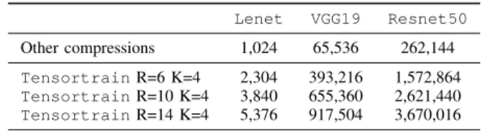
Lenet VGG19 Resnet50 Other compressions 1,024 65,536 262,144 TensortrainR=6 K=4 2,304 393,216 1,572,864 TensortrainR=10 K=4 3,840 655,360 2,621,440 TensortrainR=14 K=4 5,376 917,504 3,670,016
TABLE I: Size of hidden layer representations for one input sample in the forward propagation step of various deep models using TT layer decomposition. Tensortrain is the only com-pression strategy that induces such an inflation of each sample size during execution. Values correspond to data sample from the MNIST dataset for Lenet and CIFAR100 for VGG19 and Resnet50.
Some techniques based on inducing sparsity in neural connections, e.g. zeroing single weights in layer tensors, can be seen as particular cases of our method. The simplest approach is to remove the weights with lowest magnitude
until a given sparsity ratio is reached, followed by finetuning. Such method can be seen as the particular case of ours when only one factor is used to approximate weight matrices, i.e. Q = 1. In the experiment section, we show that this method does not allow high compression rate without significant degradation of the accuracy. The work [17] similarly proposes to iteratively remove connections and finetune the remaining weights, achieving better classification performance. Others sparsity inducing techniques exist [18], [19], however these do not seem to offer much improvements in general settings [20].
The idea of replacing layers by sparse factorization is also explored for specific structures. Deep Fried Convnets [21] propose to replace dense layers of convolutional neural networks by the Fastfood approximation [22]. This ap-proximation is a product of diagonal matrices, a permutation matrix, and a Hadamard matrix, which can itself be expressed as a product of log D sparse matrices [11]. Fastfood approximation [21] thus provides a product of sparse factors that is a particular and a more constrained case of our general framework. In fact, the Hadamard matrix imposes a strong structural constraint on the factorization, which might not be suitable for all layers of a deep architecture.
The term sparse decomposition used in [23] for network compression refers to products between dense and sparse matrices to represent the weights of the convolution kernels in a network. Finally, the work [24] proposes a similar framework to ours, along with a regularization strategy to learn the sparsity in the sparse factors. However, the method does not allow for more than two sparse factors and the compression of the convolutional layers is not considered reducing its scope and applicability.
III. EXPERIMENTS
Section III-A details the experimental settings and parame-ters to ensure reproducibility. We provide an in depth analysis of our method in Section III-B. Finally, we compare our method with state-of-the-art baselines in Section III-C. A. Experimental settings
The analysis focuses on the image classification task. We in-vestigate the compression of standard architectures (pretrained models) with our approach and with a few state of the art methods. All methods are evaluated by measuring both the compression ratio and the accuracy of compressed models. We first provide implementation details and datasets details, then we present the baselines and the hyperparameters chosen to make the comparison as fair as possible.
a) Datasets and investigated Architectures: Experiments are performed on four standard image classification datasets of varying difficulty: MNIST [25], SVHN [26], CIFAR10, CIFAR100 [27]. We investigate compression of few famous architectures including Lenet [25], VGG19 [28], Resnet20 and Resnet50 [29]. Details on datasets and neural architec-tures may be found in Table II.
b) Competing baselines: Baselines and variants of our approach are now presented. In all cases the methods are applied on the same pre-trained models and all compressed models are fine-tuned after compression. The following meth-ods are evaluated:
• Low-rank factorization methods, including Tensor-Train decomposition [7], [15] (TT) and a hybrid method that we propose exploiting Tucker decomposition [6] for the compression of convolutional layers and SVD [3] for dense layers (Tucker-SVD).
• Two different sparsity inducing pruning techniques. The first one is a simple magnitude based projection of weight matrices on a sparse support. This method is a particular case of our model where only one sparse factor is required and is named “Hard pruning” (HP). The second method, named Iterative pruning (IP) is the iterative strategy proposed in [17], which refines magnitude based projection with finetuning steps.
• Our method PSM (i.e. Algorithm 1 with palm4MSA as the compresion algorithm) and two variants designed to gain more insight on its behaviour:
– PSM random: A sparse factorization with random sparsity support and weights randomly initialized using the procedure described in Section III-A; – PSM re-init: The sparsity support is obtained
by running Palm4MSA but the weights are ran-domly reset following the procedure described in Section III-A.
Note that we did not include Deep Fried convnets in our comparison, since this method is built to compress only fully connected layers. Our attempts to apply Deep Fried to convolutional layers yielded poor results, making the method unusable on most state of the art architectures.
c) Hyper-parameters: We looked for fair comparison by choosing hyper-parameters according to literature if available else by grid search.
Palm4MSAalgorithm: the stopping criteria is the same as [13]: 300 iterations or a relative change between two iterations below 10−6. We use the projection method from [12]. With K being the desired level of sparsity, the method ensures that on average each sparse factor contains at least K non-zero values per row and per column and at most 2K.
Tensor-Train decomposition: we chose M = 4 cores for the decomposition of any tensor, which offers the best perfor-mance/compression trade-off in the original paper [7]. In the experiments, various maximum rank values R are evaluated.
Hybrid Tucker and SVD decomposition: the rank of the Tucker decomposition is automatically detected by the Vari-ational Bayes Matrix Factorization method (VBMF), as ex-plained in [6]. The rank of the SVD in the dense layers is chosen such that only a certain percentage (specified in the experiments) of the singular values are kept.
Fine-tuning: Lenet network is finetuned with the RMSProp optimizer and 100 learning epochs. VGG19 and
Nom Input shape # classes Train size Validation size Test size NN models MNIST (28 × 28 × 1) 10 40 000 10 000 10 000 Lenet
SVHN (32 × 32 × 3) 10 63 257 10 000 26 032 VGG19 CIFAR10 (32 × 32 × 3) 10 50 000 10 000 10 000 VGG19
CIFAR100 (32 × 32 × 3) 100 50 000 10 000 10 000 VGG19, Resnet50, Resnet20
TABLE II: Datasets: attributes and investigated NN models.
Resnet networks are fine-tuned with Adam [30] optimizer and 300 and 200 epochs respectively. For each compression method and configuration, the best learning rate is chosen using the classification error on a validation sample after 10 iterations, with learning rate values in {10−3, 10−4, 10−5}. Standard data augmentation is applied: translation, rotation and flipping of the images.
d) Implementation details: The code is written in Python, including the palm4MSA algorithm (the code is available on github12). NNs are implemented with Keras [31] and
Tensorflow[32]. Due to the lack of efficient implementa-tion of computaimplementa-tion with sparse matrices in Tensorflow, we had to redefine the implementations of the dense matrix product and convolution from Keras.
To implement PSM-convolution layers, we rebuild the con-volution kernel from the product of sparse matrices. Then this convolution kernel is directly used as a weight tensor in the Tensorflow function conv2d for fast computation. When needed, the initialization of the weights of PSM layers must be adapted to the reduced number of connections in the layer. We thus adapt the initializations Xavier [33] and He[34] to the initialization of sparse matrices. Specifically, the first sparse factor is initialized using the He method because ReLU activation function is applied yielding not zero-centered values. The subsequent sparse factors are initialized using the Xavier method since the absence of non-linearity between factors make the inner-activations be zero-centered.
The TT decomposition is performed by applying the de-composition function matrix_product_state, provided by the Tensorly library [35], on the tensors obtained on the pre-trained networks.
To implement the iterative pruning method from [17], the prune_low_magnitude function from the library tensorflow_model_optimization [32] is used. With this method, the pruning and the refinement of weights are combined by progressively removing the connections during the learning process until the desired percentage of pruning is obtained.
B. Analysis of the method
We first provide an in-depth analysis of our method to validate the use of Palm4MSA for the decomposition of layer’s weight matrices into products of sparse matrices. Then, we study the impact of hyper-parameters Q and K on model accuracy and on compression rate.
1Code for the PSM-nets project: https://github.com/lucgiffon/psm-nets 2Code for the Palm4MSA algorithm: https://github.com/lucgiffon/qkmeans
Vgg19 Resnet20 Resnet50 Base 0.67 0.73 0.76 PSM Q=2 K=2 0.46 0.56 0.67 PSM re-init. Q=2 K=2 0.42 0.53 0.57 PSM random Q=2 K=2 0.44 0.48 0.41 PSM Q=2 K=14 0.64 0.69 0.72 PSM re-init. Q=2 K=14 0.57 0.63 0.63 PSM random Q=2 K=14 0.58 0.62 0.62 PSM Q=3 K=2 0.42 0.57 0.67 PSM re-init. Q=3 K=2 0.32 0.48 0.51 PSM random Q=3 K=2 0.39 0.29 0.47 PSM Q=3 K=14 0.62 0.70 0.72 PSM re-init. Q=3 K=14 0.31 0.60 0.58 PSM random Q=3 K=14 0.51 0.60 0.59
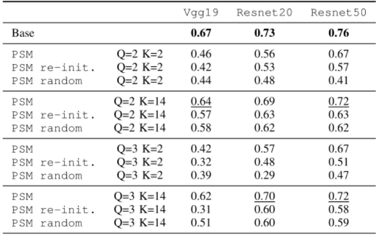
TABLE III: Classification performance on CIFAR100 ob-tained with neural network models compressed by 3 variations of layer decomposition into sparse matrix products: PSM, PSM re-init, and PSM random. Q is the number of factors in the decomposition, K the sparsity level.
Fig. 3: Relative error approximation by layers using Palm4MSA for VGG19 architecture pre-trained on the CIFAR100 dataset. "C" stands for "Conv2D", "D" for "Dense" and "S" for "Softmax". "C1", correspond to the first layer of the network then the layers are ordered from left to right until the last fully connected layer "S".
a) Approximation error: The quality of the Palm4MSA approximation of the original weight matrices is evaluated, as well as its influence on the final performance of the method. We report results obtained on the compression of VGG19 trained on CIFAR100 as an illustration. Figure 3 shows the approximation error between the product of Q sparse factors
˜
W :=QQ
layer. The error is computed as the normalized Froebenius distance between the original and the approximated matrices: error = kW − ˜Wk2
F/kWk2F.
We observe that the approximation error of palm4MSA algorithm may be quite high for some of the layers. Yet looking at Table III, we observe that the fine tuning step allows recovering original accuracy (i.e. the one of the uncompressed network) in most cases. Figure 3 further shows that a higher K, (i.e. the minimum number of non-zero values per row and per column) yields better approximation and usually a better accuracy as well (see Table III).
High approximation errors in Figure 3 suggest that Palm4MSA may not be well adapted for the task. In order to investigate this deeper, we provide results for two variants of our methods: PSM-random and PSM-reinit methods. More precisely, we want to evaluate (I) the relevance of the sparsity support found by Palm4MSA through comparison of our approach to PSM-random and (II) the relevance of the learned weights by comparing our approach to PSM-reinit. The results reported in Table III show first that the network compressed using the Palm4MSA method obtains the best performance in classification with all the tested combina-tions of sparsity level K and number of factors Q. Overall PSM-reinitand PSM-random perform significantly worse than our main approach and most of the time reach similar results.
This finally reinforce the idea that palm4MSA is able to recover some unknown underlying structure in the weight matrices even though the overall approximation error is high. b) Sparsity level and the number of factors: Figure 4 and Table III show the performance of our models obtained with various sparsity levels K and numbers of factors Q. We observe that the number of factors seems to have a rather limited effect on the quality of the performance, while sparsity level is a more determining factor of the quality of the approximation.
C. Comparative study
Figure 4 reports comparative results obtained on standard benchmark datasets with well known architectures. The main observations are now presented.
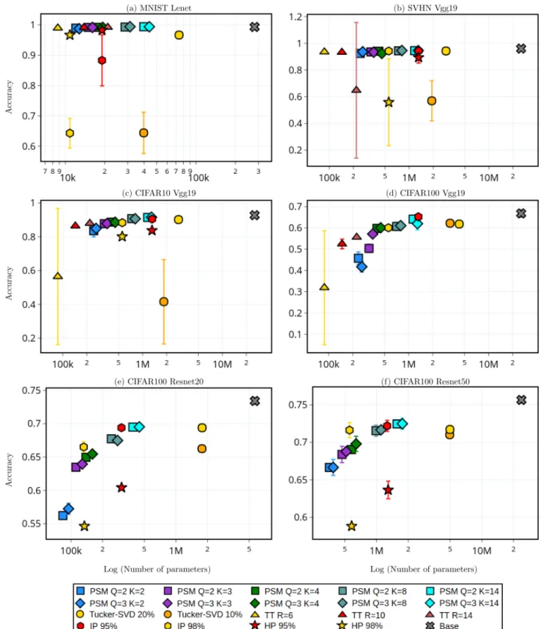
a) Reliability: First of all, the behaviour of the baseline methods seems to depend on the experiment. For instance, TT performance varies depending on the chosen rank, see rank 10 in figure 4-(b). Iterative Pruning technique performs badly on MNIST. Moreover, these baselines are not always manageable in practice, e.g. no results are available for TT on Resnet compression, see below. On the contrary, we observe more stable performances with regards to the choice of hyper-parameters and a systematic very low variance for our method. b) Comparison to low rank decomposition techniques: Our approach significantly outperforms the Tucker-SVD method in any case. Indeed, this low rank decomposition meth-ods cannot reach high compression regime, without degra-dation of the accuracy of the network. On the contrary, the TT formulation can achieve higher compression rates than
Tucker, as observed in past works. TT offers better results than Tucker decomposition and performs similarly or above our method in some cases. Yet, the method has drawbacks. First, very strong variance is observed in several cases, especially for high compression rates (see results in figures (b) to 4-(d) on SVHN, CIFAR10-100). Second, the implementation provided by authors does not provide any results, when the product of the number of filters and the TT rank is large. In particular, we are unable to run experiments on models such as Resnet20 and Resnet50 because the memory footprint is increased considerably to the extent that the batch become impossible to store in memory during the execution of the wider convolutional layers of these networks (Table I and figures 4-(e) and 4-(f)).
c) Comparison with pruning techniques: In the “Hard” pruning case, the compressed network perform very poorly. This confirms that a sparse factorization with more than one factor is beneficial. When applying the procedure of [17], however, the magnitude based pruning method conserves good accuracy while removing up to 98% of the connections from the model, except for the MNIST dataset. While our approach significantly outperforms the Hard pruning technique in any case, Iterative pruning [17] can lead to significantly higher performance compression in high compression settings than our approach, this is particularly the case with Resnet models on CIFAR100 (figures 4-(e) and 4-(f)). In other settings on Resnet and for compressing other models, this technique has similar performance vs compression trade-off to our method. Since the Hard pruning technique can be viewed as a special case of our method, results suggest that an iterative-like extension of our method could reach even better results, which is a perspective of this work.
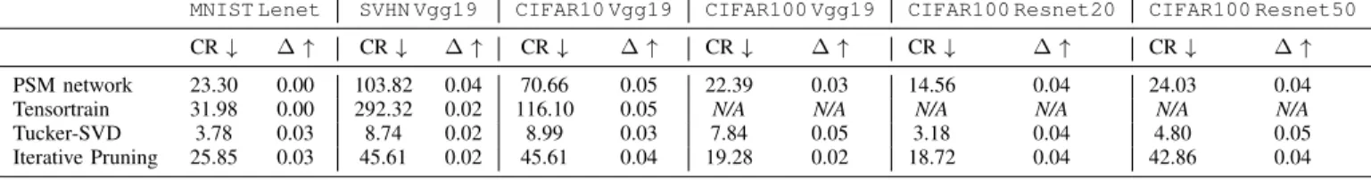
d) Compression rates that preserve accuracy: Table IV displays the highest compression rates obtained with the dif-ferent methods while preserving the accuracy with a maximum of 5 percents decrease in accuracy. The main observations are:
• Our approach PSM-net significantly outperforms the Tucker-SVDin any case.
• Our method may compete with the tremendous
compres-sion rates obtained with Tensor-train observed on small to medium scaled problems, i.e. small architectures (e.g. LeNet) or bigger architectures (e.g. VGG19) trained on simple data (hence enabling strong compression rates).
• On larger scaled problems the Tensor-train method could not reach an accuracy below 5 percents, this is why N/A is reported in some cases, since it would have required using higher TT ranks but this caused memory overflow problems (see Section II-C). On such cases our approach allows reaching up to ×20 compression rates.
• The PSM-nets are comparable with the Iterative Pruningapproach, yielding higher compression rate in the case of the VGGG19 networks but lower for Resnet ones.
Fig. 4: Accuracy (y-axis) as a function of the log of the number of parameters (x-axis) for compressed versions of standard pretrained models on several datasets, obtained with various compression methods. The number of parameters include dense and convolutional layers weights only. The PSM models have Q sparse factors with a sparsity level K. The Tucker-SVD hybrid uses 10% or 20% of the singular values in dense layers. The R value for Tensortrain (TT) method refers to the maximum rank of the cores in the decomposition. Note that the TT method requires too much memory to obtain any result on the Resnet architectures. Finally, the Iterative Pruning (IP) and Hard pruning (HP) approaches prune 95% or 98% of the Base’s number of weights. Base stands for the uncompressed pretrained model.
MNIST Lenet SVHN Vgg19 CIFAR10 Vgg19 CIFAR100 Vgg19 CIFAR100 Resnet20 CIFAR100 Resnet50 CR ↓ ∆ ↑ CR ↓ ∆ ↑ CR ↓ ∆ ↑ CR ↓ ∆ ↑ CR ↓ ∆ ↑ CR ↓ ∆ ↑ PSM network 23.30 0.00 103.82 0.04 70.66 0.05 22.39 0.03 14.56 0.04 24.03 0.04 Tensortrain 31.98 0.00 292.32 0.02 116.10 0.05 N/A N/A N/A N/A N/A N/A Tucker-SVD 3.78 0.03 8.74 0.02 8.99 0.03 7.84 0.05 3.18 0.04 4.80 0.05 Iterative Pruning 25.85 0.03 45.61 0.02 45.61 0.04 19.28 0.02 18.72 0.04 42.86 0.04
TABLE IV: Summary of the compression rates (CR) and accuracy loss (∆) for different compression strategies. The highest compression rates are reported for a loss (with respect to the accuracy of the uncompressed model) below 0.05 accuracy. Values are not available for Tensor-train on CIFAR100 because such results would require too large TT ranks that yield memory inflation.
IV. CONCLUSION
This paper presents a new approach to compress dense and convolutional layers of a pretrained neural network. Our method is based on the decomposition of weight matrices into products of sparse matrices. Unlike common decomposition methods, our method does not make any assumptions on the rank of the weight matrices and allows high compression rates while maintaining accuracy. For instance, we were able to compress a VGG19 network around 30×, or a Resnet50 network 20×, while losing only 1 to 5 percents of accuracy.
ACKNOWLEDGMENT
This work was funded in part by the French national research agency (grant number ANR16-CE23-0006). This work was performed using HPC resources from GENCI-IDRIS (Grant 2020-AD011011766)
REFERENCES
[1] B. Neyshabur, Z. Li, S. Bhojanapalli, Y. LeCun, and N. Srebro, “The role of over-parametrization in generalization of neural networks,” in ICLR, 2018.
[2] Y. Cheng, D. Wang, P. Zhou, and T. Zhang, “A survey of model compression and acceleration for deep neural networks,” IEEE Signal Processing Magazine, 2017.
[3] T. N. Sainath, B. Kingsbury, V. Sindhwani, E. Arisoy, and B. Ramabhad-ran, “Low-rank matrix factorization for Deep Neural Network training with high-dimensional output targets,” in ICASSP. IEEE, 2013, pp. 6655–6659.
[4] E. L. Denton, W. Zaremba, J. Bruna, Y. LeCun, and R. Fergus, “Exploiting linear structure within convolutional networks for efficient evaluation,” in NIPS, 2014, pp. 1269–1277.
[5] V. Lebedev, Y. Ganin, M. Rakhuba, I. Oseledets, and V. Lempit-sky, “Speeding-up convolutional neural networks using fine-tuned CP-decomposition,” in ICLR, 2015.
[6] Y.-D. Kim, E. Park, S. Yoo, T. Choi, L. Yang, and D. Shin, “Compression of Deep Convolutional Neural Networks for Fast and Low Power Mobile Applications,” in ICLR, 2016.
[7] A. Novikov, D. Podoprikhin, A. Osokin, and D. Vetrov, “Tensorizing Neural Networks,” in NIPS, 2015.
[8] S. Anwar, K. Hwang, and W. Sung, “Structured pruning of deep convolutional neural networks,” ACM Journal on Emerging Technologies in Computing Systems (JETC), vol. 13, no. 3, pp. 1–18, 2017. [9] Z. Liu, M. Sun, T. Zhou, G. Huang, and T. Darrell, “Rethinking the
Value of Network Pruning,” in ICLR, 2018.
[10] Y. Guo, “A survey on methods and theories of quantized neural net-works,” arXiv preprint arXiv:1808.04752, 2018.
[11] T. Dao, A. Gu, M. Eichhorn, A. Rudra, and C. Ré, “Learning Fast Al-gorithms for Linear Transforms Using Butterfly Factorizations,” vol. 97. PMLR, 2019, pp. 1517–1527.
[12] L. L. Magoarou and R. Gribonval, “Flexible Multi-layer Sparse Approx-imations of Matrices and Applications,” IEEE Journal of Selected Topics in Signal Processing, vol. 10, no. 4, pp. 688–700, 2016.
[13] L. Giffon, V. Emiya, L. Ralaivola, and H. Kadri, “QuicK-means: Acceleration of K-means by learning a fast transform,” hal preprint, 2019.
[14] J. Wang, Y. Chen, R. Chakraborty, and S. X. Yu, “Orthogonal convolu-tional neural networks,” in CVPR, 2020.
[15] T. Garipov, D. Podoprikhin, A. Novikov, and D. Vetrov, “Ultimate tensorization: compressing convolutional and fc layers alike,” NIPS workshop, 2016.
[16] T. Garipov, “Github Tensorizing Neural Networks,” 2020. https: //github.com/timgaripov/TensorNet-TF
[17] M. Zhu and S. Gupta, “To prune, or not to prune: Exploring the efficacy of pruning for model compression,” in ICLR, 2017.
[18] D. Molchanov, A. Ashukha, and D. Vetrov, “Variational Dropout Spar-sifies Deep Neural Networks,” in ICML, 2017.
[19] C. Louizos, M. Welling, and D. P. Kingma, “Learning Sparse Neural Networks through $L_0$ Regularization,” in ICLR, 2018.
[20] T. Gale, E. Elsen, and S. Hooker, “The State of Sparsity in Deep Neural Networks,” in Work. on Device Machine Learning & Compact Deep Neural Network Representations (ODML-CDNNR), 2019.
[21] Z. Yang, M. Moczulski, M. Denil, N. de Freitas, A. Smola, L. Song, and Z. Wang, “Deep Fried Convnets,” in ICCV, 2015.
[22] Q. Le, T. Sarlós, and A. Smola, “Fastfood — Approximating Kernel Expansions in Loglinear Time,” in ICML, 2013, p. 9.
[23] B. Liu, M. Wang, H. Foroosh, M. Tappen, and M. Pensky, “Sparse convolutional neural networks,” in CVPR, 2015, pp. 806–814. [24] K. Wu, Y. Guo, and C. Zhang, “Compressing deep neural networks with
sparse matrix factorization,” IEEE Transactions on Neural Networks and Learning Systems, 2019.
[25] Y. LeCun, L. Bottou, Y. Bengio, and P. Haffner, “Gradient-based learning applied to document recognition,” Proceedings of the IEEE, vol. 86, no. 11, pp. 2278–2324, 1998.
[26] Y. Netzer, T. Wang, A. Coates, A. Bissacco, B. Wu, and A. Y. Ng, “Read-ing Digits in Natural Images with Unsupervised Feature Learn“Read-ing,” in NIPS, 2011, p. 9.
[27] A. Krizhevsky, I. Sutskever, and G. E. Hinton, “Imagenet classification with deep convolutional neural networks,” NIPS, vol. 25, pp. 1097–1105, 2012.
[28] K. Simonyan and A. Zisserman, “Very Deep Convolutional Networks for Large-Scale Image Recognition,” in ICLR, 2015.
[29] K. He, X. Zhang, S. Ren, and J. Sun, “Deep Residual Learning for Image Recognition,” in CVPR. IEEE, 2016, pp. 770–778.
[30] D. P. Kingma and J. Ba, “Adam: A method for stochastic optimization,” in ICLR, 2015.
[31] F. Chollet. (2015) Keras: The Python deep learning API. https://keras.io/ [32] M. Abadi, A. Agarwal, P. Barham, E. Brevdo, Z. Chen, C. Citro, G. S. Corrado, A. Davis, J. Dean, M. Devin, S. Ghemawat, I. Goodfellow, A. Harp, G. Irving, M. Isard, Y. Jia, R. Jozefowicz, L. Kaiser, M. Kudlur, J. Levenberg, D. Mané, R. Monga, S. Moore, D. Murray, and et al., “TensorFlow: Large-scale machine learning on heterogeneous systems,” 2015. https://www.tensorflow.org/
[33] X. Glorot and Y. Bengio, “Understanding the difficulty of training deep feedforward neural networks,” in AISTATS, 2010, pp. 249–256. [34] K. He, X. Zhang, S. Ren, and J. Sun, “Delving Deep into Rectifiers:
Surpassing Human-Level Performance on ImageNet Classification,” in ICCV, 2015.
[35] J. Kossaifi, Y. Panagakis, A. Anandkumar, and M. Pantic, “Tensorly: Tensor learning in python,” JMLR, vol. 20, no. 26, pp. 1–6, 2019.