Improved resistive shunt by means of negative capacitance: new circuit, performances and multi-mode control

HAL Id: hal-01392666

https://hal.archives-ouvertes.fr/hal-01392666

Submitted on 4 Nov 2016

HAL is a multi-disciplinary open access

archive for the deposit and dissemination of

sci-entific research documents, whether they are

pub-lished or not. The documents may come from

teaching and research institutions in France or

abroad, or from public or private research centers.

L’archive ouverte pluridisciplinaire HAL, est

destinée au dépôt et à la diffusion de documents

scientifiques de niveau recherche, publiés ou non,

émanant des établissements d’enseignement et de

recherche français ou étrangers, des laboratoires

publics ou privés.

Improved resistive shunt by means of negative

capacitance: new circuit, performances and multi-mode

control

Marta Berardengo, Olivier Thomas, Christophe Giraud-Audine, Stefano

Manzoni

To cite this version:

Marta Berardengo, Olivier Thomas, Christophe Giraud-Audine, Stefano Manzoni. Improved resistive

shunt by means of negative capacitance: new circuit, performances and multi-mode control. Smart

Materials and Structures, IOP Publishing, 2016, 25, pp.075033. �10.1088/0964-1726/25/7/075033�.

�hal-01392666�

Improved resistive shunt by means of

negative capacitance: new circuit,

performances and multi-mode control

M Berardengo

, O Thomas

, C Giraud-Audine

and S Manzoni

1_{Politecnico di Milano—Department of Mechanical Engineering, Via La Masa, 34-20156 Milan, Italy} 2

Arts et Métiers ParisTech, LSIS UMR CNRS 7296, 8 bd. Louis XIV, 59046 Lille, France 3

Arts et Métiers ParisTech, L2EP, 8 bd. Louis XIV, 59046 Lille, France E-mail:marta.berardengo@polimi.it

Abstract

This paper deals with vibration control by means of piezoelectric patches shunted with electrical impedances made up by a resistance and a negative capacitance. The paper analyses most of the possible layouts by which a negative capacitance can be built and shows that a common mathematical description is possible. This allows closed formulations to be found in order to optimise the electrical network for mono- and multi-mode control. General analytical formulations are obtained to estimate the performance of the shunt in terms of vibration reduction. In particular, it is highlighted that the main effect of a negative capacitance is to

artificially enhance the electromechanical coupling factor, which is the basis of performance

estimation. Stability issues relating to the use of negative capacitances are especially addressed

using refined models for the piezoelectric patch capacitance. Furthermore, a new circuit based on

a couple of negative capacitances is proposed and tested, showing better performances than those provided by the usual layouts with a single negative capacitance. Finally, guidelines and analytical formulations to deal with the practical implementation of negative capacitance circuits are provided.

Keywords: piezoelectric shunt, negative capacitance, vibration control, damping, smart structure (Some figures may appear in colour only in the online journal)

1. Introduction

The use of piezoelectric actuators shunted with electric impedances in order to damp structural vibrations is an attractive approach because such lightweight control devices do not cause high load effects and require little or no power supply to control the structure. Such control methods can be

classified as passive if the electric components used to

prac-tically build the impedance are passive (e.g. composed of a

single resistance (resistive (R) shunt) or the series of a

resistance and an inductance(resonant (RL) shunt)) [1],

semi-passive if the electronic circuit needs to be powered but is still

theoretically equivalent to a passive one (in the case of a

synthetic inductance, for instance) [2], or active. The most

common example of an active circuit in the context of

piezoelectric shunt is the negative capacitance (NC),

practi-cally realised with an operational amplifier (OP-AMP). The

use of NCs enables the attenuation performance of the shunt

to be increased [3, 4], but poses some issues relating to

possible instabilities in the electro-mechanical system(EMS)

because of its active nature.

Some aspects relating to the use of NCs to enhance the performances of shunted piezoelectric actuators have been addressed in the literature. Indeed, the use of circuits based on OP-AMPs to shunt piezoelectric actuators has been described

in different pieces of work (e.g. [5]). Among the different

circuits proposed, the NC was shown to be effective for

vibration control. De Marneffe and Preumont[3] analysed the

simplest layouts, named ideal circuits(IC) here, to build the

have focused on more complex circuits, named real circuits (RC) here, because they are more reliable for practical implementation. The RCs cannot be considered as pure NCs

(see section 5) but as complex negative impedances, while

ICs can be seen as pure NCs. Behrens et al[4] considered an

RC and showed its capability to provide broadband vibration attenuation when shunted to piezoelectric actuators. Park and Baz[6] shunted a pair of interdigital electrode piezoceramics

with an NC to achieve broadband vibration control for a cantilevered beam. The works of Behrens et al and of Park and Baz differ in how to shunt the NC to the piezoelectric element(series and parallel respectively). Manzoni et al [7]

analysed the stability of an RC in a series layout and Kodejška et al [8] used an RC in a series configuration in an

adaptive circuit for the purpose of vibration isolation. Beck et al proposed an electrical model of an RC in a series layout in[9] and presented a procedure for improving the attenuation

performance provided by an RC in a series configuration

in[10].

An NC can be coupled to any passive(or semi-passive)

shunt in order to increase its performance—especially the

traditional R- and RL-shunts. The latter solution allows the attenuation provided by the pure resistive shunt to be

improved a lot, despite losing its robustness [11]. The idea

followed in this article is to use a negative capacitance to increase the attenuation performance of a pure resistive shunt while keeping its robustness. This article also addresses a tuning strategy to obtain multi-mode attenuation by means of a negative capacitance resistive shunt, whereas vibration attenuation is localised in a narrow frequency band around a given resonance for traditional R and RL shunts.

One of the purposes of the paper is to propose and

analyse a new shunt impedance configuration based on two

NCs, in order to enhance the performance of traditional NC circuits coupled to a resistive shunt. In doing so, traditional layouts for NCs are reconsidered here. Indeed, although the use of an NC with a resistive shunt has already been described in the literature, no clear criteria for tuning the electric para-meters and optimising shunt performance are available. Fur-thermore, different layouts can be used to practically build an NC circuit as mentioned previously, and some of them are seldom taken into account or analysed in the literature. Finally, no clear evaluation of the possible performances attainable with a negative capacitance are available. There-fore, for all the above-mentioned issues, the main targets of this paper are(i) to analyse most of the possible practical NC

configurations, showing that a common analytical treatment

can be used(see section2); (ii) to propose a refined model for

piezoelectric patch capacitance in order to derive accurate stability limits when NCs are used and to achieve a more

accurate description of EMS behaviour (refer to sections 2

and6); (iii) to propose a new layout based on the use of two

NCs able to guarantee better vibration attenuation with respect to the traditional NC layouts (see section 3); (iv) to

provide clear optimisation formulas to be employed in order to reach the highest possible attenuation for both mono-modal

and broadband attenuation and (v) to derive analytical

for-mulas which foresee the attenuation performance of the shunt,

valid for any NC configuration (refer to section 4); finally,

(vi) to study the behaviour of RCs and compare it to that of

ICs, for practical implementations (see section 5). To

con-clude, all the aforementioned theoretical results are validated by experiments(refer to section6).

2. Model of the electro-mechanical system 2.1. Governing equations

The model employed to describe the behaviour of the EMS is the one presented in the paper of Thomas et al[2], which was

used by its authors to find the optimal tuning of R and RL

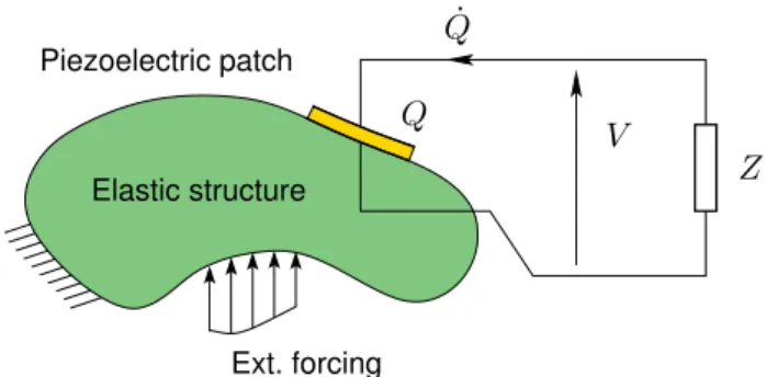
impedances shunted to a piezoelectric actuator as well as the associated vibration attenuation performances. We consider an arbitrary elastic structure with one piezoelectric patch

bonded to it and excited by an external force (named Fext),

shown in figure 1. An arbitrary shunt impedance Z is

con-nected to the piezoelectric patch and V is the voltage between the electrodes of the piezoelectric actuator, which is also the shunt terminal voltage. Q is the electric charge in one of the electrodes, and considering the convention of the sign for V in

figure1, Q is precisely the charge in the upper electrode. A

reduced order model can be obtained by expressing the

dis-placement U x t( , ) at any point x and time t in modal

coor-dinates and considering the N vibration eigenmodes(N being

infinite in theory):

å

where Fiis the ith eigenmode of the structure(normalised to

the unit modal mass) and qiis the ith modal coordinate. The

modal coordinates qi(t) are the solutions to a problem of the form[12,13]: x w w c + + - = " Î q¨i 2 i i iq˙ i2qi iV Fi i 1 ...N (2a)

å

In the above equations, widenotes the ith natural frequency of

the EMS in short circuit (SC, i.e. with Z = 0), x_i is the ith

structural damping factor, Fi is the harmonic modal forcing

term, C¥ is the electrical capacitance of the piezoelectric

patch(its physical meaning will be discussed in section2.2)

Figure 1.An arbitrary structure with a piezoelectric patch connected

and c_iis the modal coupling coefficient, which represents the energy transfer between the ith mode shape and the piezoelectric patch. The values of c_idepend on the electrical, geometrical and mechanical characteristics of the piezo-electric actuator and structure, and on the position of the

actuator. These c_i coefficients can be computed analytically

[12] or by a finite element model [13], or estimated

experimentally. The writing of equation (2a) relies on a

chosen normalisation of the mode shapes to have unit modal masses. The unit of Fi is therefore kg-1 2, the unit of qi is m·kg1 2_{, and the one of F}

iis N·kg-1 2, so that the unit of ciis

either N·V-1·kg-1 2or C·m-1·kg-1 2, depending on whether the direct or converse piezoelectric effects are considered.

Note that (Fi, wi) are the eigenmodes of the EMS with the

piezoelectric patch in short circuit(SC) (with V = 0) and that

¥

C is the patch capacitance of the blocked structure (with

= "  = "

U x t( , ) 0 x qi 0 i). As for a rectangular

piezo-electric patch with a constant thickness h, the patch capacitance of the blocked structure can be computed theoretically by[13]:

 =

¥

C ¯33S h ( )3 where S is the area of the electrodes and¯33 is the modified

dielectric permittivity at constant strain, in the patch transverse direction, of the piezoelectric material.

The EMS is thus described by N modal equations

(equation (2a)), corresponding to the balance law of

mechanical forces, which describe the equations of motion of the EMS. These equation(2a) are coupled by the term c V_i to equation(2b), which represents the electrical behaviour of the

system. Equation (2b) is related to the balance of electric

charges on the piezoelectric patch electrodes.

2.2. Model of the electrical capacitance and static correction The piezoelectric actuator and the structure are physically linked, and thus the dynamics of the structure is affected by the electrical behaviour of the EMS through the coupling coefficients c_i. On the other hand, the electrical behaviour of the system is in turn affected by the dynamics of the structure. Indeed, the expression of an equivalent capacitance can be derived from equations(2a), (2b). The expression of such an

equivalent capacitance is frequency- dependent and can be obtained solving equation (2a) with respect to qi in the

fre-quency domain (with Fi = 0) and substituting the result in

equation(2b). If all variables oscillate at a frequency Ω, the

equivalent capacitance of the EMS is:

å

where j is the complex imaginary unit and Q and V are the complex amplitudes of Q and V.

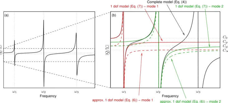
The trend of C( )W = Q V for a generic system is

depicted in figure 2(a). It shows that the value of C ( )W

decreases after each resonance of the system, because of the

second term of equation(4). As for the high frequency range

(at frequencies above the highest natural frequency of the EMS),C( )W C¥. As a consequence, the capacitanceC¥of

the blocked structure, which naturally appears in the model (2a), (2b) (see equation (3)), is also the value of the

capaci-tance of the piezoelectric patch at high frequency. In the low

frequency range, below the first natural frequency of the

EMS,C( )W C0 with:

å

If the natural frequencies of the modes are well separated, a single-degree-of-freedom approximation can be carried out

to describe the behaviour of the EMS forW wi. Therefore,

the second term of equation (4) can be approximated by

keeping only the contribution of the ith mode in the sum, so that: w c w x w W  W + - W + W " = ¼ ¥  C C j i N 2 , 1 6 i i i i i 2 2 2 ( ) ( )

This simple one-degree-of-freedom (dof) model is not

accurate in describing the behaviour of the capacitance

around the mode considered (see figure 2(b)). It can be

corrected by adding the low and high frequency contributions of all the modes which are out of the frequency band of interest. At the frequencies Ω around wi, the contribution of

all the modes n at a lower frequency (wnwi) is zero

because the corresponding term in the sum of equation (4)

tends to zero for W wn. All the modes n of higher

frequency (wnwi) contribute with a static component

c w_n2 _n2_{, since in this case W w}

n. As a consequence, a

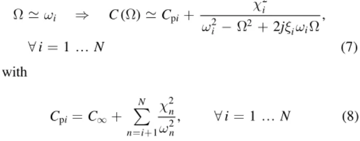
refined one-degree-of-freedom model forC ( ) is:W

w c w x w W  W + - W + W " = ¼  C C j i N 2 , 1 7 i i i i i i p 2 2 2 ( ) ( ) with

å

In other words, the capacitance value Cpiat a given frequency

does not depend on the modes of the structure at lower frequency, but just on those at higher frequency.

As a consequence, a refined one-degree-of-freedom

model of the EMS, valid in a frequency band around a given resonance(W wi), is obtained by keeping only the ith mode

in the expansion( =qn 0, " ¹n i). Therefore, equation (1) is

replaced by U x t( , ) =F x q ti( ) ( ), equationi (2a) is kept and

equation(2b) is replaced by:

c

- + =

C Vpi Q i iq 0, ( )9 where the static correction due to the higher modes is included in the term Cpi.

Figure 2(b) shows how it is possible to improve the

accuracy of the model of the capacitance using equation(7) in

place of equation(6) in the frequency band around the mode

(equation (7)) leads to a 1 dof model which almost merges

with the complete model of equation (4) around a given

resonance; this is far from being the case for the classical simple model of equation(6) withC¥. Figure2(b) also shows

thatC ( ) assumes the value CW pialmost midway between the

resonance frequencies of mode i and +i 1.

2.3. Coupling factor

In order to introduce the electromechanical coupling factor, we apply the following changes of variables:

= = V V C Q Q C , 10 i i p p ¯ ¯ _{( )}

Substituting equation (10) into equations (2a) and (9), a

normalised formulation to describe the EMS behaviour is obtained: x w w w + + - = q¨_i 2 _{i i i}q˙ i2qi i ik V¯ Fi, (11a) x w w w + + - = q¨i 2 i i iq˙ ˆi2qi i ik Q¯ Fi, (11b) w - + = V¯ Q¯ i i ik q 0, (11c) where: c w w w = = + k C , and 1 k . 12 i i i i i i i p 2 ˆ ( )

Equations(11a) and (11b) are equivalent, both expressing the

converse piezoelectric effect, as a function of either V¯ or Q¯. Equation(11b) is obtained by substituting V¯ in favour of Q¯ in

equation(11a) using (11c). The non-dimensional parameter ki

is defined as the modal electromechanical coupling factor

(MEMCF). The short- (SC) and open-circuit (OC) natural frequencies of the EMS are wiand wˆi(respectively associated

with zero (Z = 0) and infinite ( = ¥Z ) shunt impedances,

also obtained with V¯ =0 and Q¯ =0 respectively).

Equation (12) shows that the MEMCF ki is close to the ith

effective coupling factor:

w w w = - = k i i k 13 i i eff 2 2 2 ˆ ∣ ∣ ( )

As suggested in[3,14], the SC natural frequencies wiare the

poles ofC ( )W (equation (4)) and the OC natural frequencies

wˆ are its zeros. Since ki iis dimensionless, another unit for ci

isF1 2_·s-1_.

By considering the definition of ki in equation (12)

together with equation(8), it can be derived that the values of

Cpifor two consecutive modes in the spectrum are linked by:

= + + +

Cpi Cp i 1 1 ki 1 14

2

( ) ( )

Consequently, the value of the capacitance at the null frequency can be derived as a function of all the modes of the structure:

å

The following relations for the different capacitance values hold:

> > ¼ > > ¼ > ¥

C0 Cp 1 Cpi C (16) These results are illustrated infigure2(b): the capacitance, out

of the resonance zones, changes by a factor almost equal to

C kpi i2 at each resonance crossing.

Figure 2.The trend ofC( )w =∣Q V∣ for a generic, undamped three-degrees-of-freedom system.(a) The complete model of equation (4); (b)

zoom showing the complete model(black) of equation (4) and the 1 dof models of equation (6) (dashed lines) and (7) (solid lines) tuned to

mode 1(red) and mode 2 (green). Note that the continuous lines relating to equations (4) and (7) (red line, first mode) are fully superimposed

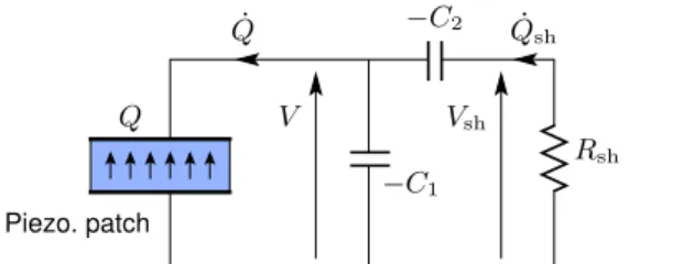
2.4. EMS with negative capacitance

Once the model of the EMS(section2.3) has been described,

we can consider the case in which an NC is connected to the piezoelectric actuator, in addition to the shunt impedance,

now denoted by Zsh. There are two classical configurations

for the NC: a parallel configuration (figure3(a)) or a series

configuration (figure3(b)). Both layouts are characterised by

the presence of an additional negative capacitance -C1 or

-C2. This element is theoretically defined by the following

relation between its terminal voltage Vcand its charge Qc(see

figure3(c)): = -V Q C 17 c c n ( )

Since NCs do not exist in nature, they are built in practice by

means of a circuit including an OP-AMP[15]. Such a circuit

will be discussed in detail in section5.

In the following, we focus our attention on the response of the EMS due to the ith vibration mode( = " ¹qn 0 n i),

using the model of equation(9) with the static correction. As

for the parallel configuration (figure3(a)), the charge Q is the

sum of the charges in the negative capacitance -C1 branch

and the shunt impedance Zsh branch, so that equation(2b) is

replaced by:

c

- - + =

Cpi C V1 Qsh i iq 0 18

( ) ( )

As for the series configuration, the voltage V is the sum of the

voltages at the terminals of the negative capacitance -C2and

the shunt impedance Zsh, so that equation(2b) is replaced by:

⎛ ⎝ ⎜ ⎞ ⎠ ⎟ c - - + = V C C Q C q 1 1 0 19 i i i i sh p 2 p ( )

In the above equations, Vsh and Qsh denote the terminal

voltage across the shunt impedance and the charge thatflows

into the shunt impedance branch, respectively.

It is now convenient to define the following equivalent

capacitances: = - = -C C C C C C C C , . 20 i i i eqp p 1 eqs p 2 2 p ( )

These are related to the configuration with -C1in parallel to

the piezoelectric patch and -C2 in series with the

piezo-electric patch respectively. By applying a change of variables analogous to that in equation (10):

= = V V C Q Q C 21 sh sh eq sh sh eq ¯ ¯ _{( )}

withCeq=CeqporCeq=Ceqs, the initial problem(11a)–(11c)

can be rewritten in the following form:

x w w w + + - = q¨i 2 i i iq˙ ( sc 2i) qi i ik V˜ ¯sh Fi, (22a) x w w w + + - = q¨i 2 i i iq˙ ( oc 2i ) qi i ik Q˜ ¯sh Fi, (22b) w - + = V¯sh Q¯sh i i ik q˜ 0 (22c)

The above set of equations defines the dynamics of the EMS

viewed from the shunt impedance Zsh since the electrical

unknowns are now V¯sh and Q¯ . The following parameterssh

have been defined: wisc and wioc are respectively the natural

frequency of the EMS with the shunt Zsh short-circuited

(Vsh=0Zsh=0) and in open-circuit (Qsh=0Zsh=

¥). Their values depend on the values of the negative

capacitances -C1and -C2. The above model characterises the

behaviour of the EMS grouped with the negative capacitances

-C1 or -C2, whose apparent capacitance is Ceqp or Ceqs,

instead of Cpi. A new coupling factor naturally appears in the

equations: the enhanced modal electromechanical coupling

Figure 3.Shunt with the addition of an NC:(a) parallel configuration; (b) series configuration. (c) Definition of an NC.

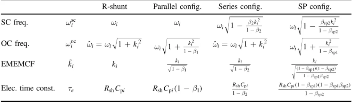
Table 1.Parameters of the EMS enhanced by a single NC in a parallel and series configuration and by two NCs for the series+parallel (SP)

configuration.

R-shunt Parallel config. Series config. SP config.

SC freq. w_isc _w i wi _{w -} c -i _{C C} 2 i i 2 2 p w -_{i +}c -C C C 2 i i 2 1 2 p OC freq. wioc w = w + c i i2 _Ci i 2 p ˆ w +i2 _Cc_-i_C i 2 p 1 w = w + c i i2 _Ci i 2 p ˆ w +i2 _Cc_-i_C i 2 p 1 EMEMCF k˜i ki -k 1 i C C i 1 p -k 1 i C i C p 2 ⎜ ⎟ ⎛ ⎝ ⎜ ⎞ ⎠ ⎟⎛_⎝ ⎞_⎠ - + -k 1 1 i C C i C C C i C 1 p 1 2 p 2 Elec. time const. te R Csh pi Rsh(Cpi-C1) R

-C -C C C sh i i p 2 2 p -+ -R C C C C C C sh i i p 1 2 1 2 p ( )

factor(EMEMCF) k˜ , that can be written as:i w w w = -ki i i , 23 i oc 2 sc 2 2 ∣ ˜ ∣ ( ) ( ) ( )

similar to that of equation(13). One can notice that k˜ is noti

exactly the traditional effective coupling factor since now the denominator is wiand not wi

sc_{. These parameters, which take}

different values in the parallel and series configurations, are

gathered in table 1. Their dependence upon the negative

capacitances C1 or C2 will be discussed in detail in

sections2.6and2.7.

It is worth highlighting that equations(22a)–(22c), which

describe the EMS with an NC(series or parallel), are valid

even for a simple shunt(without NC). Indeed, it is sufficient

to substitute in the model the original wiand wˆ in place of wi isc

and w_iocand kiin place of k˜ . Therefore, the model describedi

by equations(22a)–(22c) can be considered general and valid

for simple and NC shunts. 2.5. Resistive shunt

We now consider a resistance as shunt impedance (i.e.

=

Zsh Rsh infigure3). This leads toVsh= -R Qsh ˙ , so thatsh

equation(22c) becomes:

teQ¯˙sh+Q¯sh-wi i ik q˜ =0. (24) With the electrical time constant

t = R C .e sh eq (25)

One has to remark that tealso depends on the considered ith

mode because Ceq depends on Cpi.

Consequently, relying on equations (22b) and (24), the

frequency response function (FRF) Hi( ) between aW

harmonic modal force Fiof frequency Ω and qiis:

t w x w t t w x w t W = = + W - + W + W + - W H q F j j 1 1 2 2 26 i i i e i i i e e i i i e sc 2 2 oc 2 2 ( ) ( ) ( ) [ ( ) ] ( )

2.6. Stability conditions for ideal series and parallel circuits The introduction of active elements such as OP-AMP makes the stability analysis of the EMS compulsory. One possible approach is to apply the Routh–Hurwitz criterion [16] to the

controlled FRF. This guarantees having all poles with nega-tive real parts[17]. If we consider the FRF of a

single-degree-of-freedom EMS defined in equation (26), the stability

con-dition for the parallel configuration is found to be: <

C1 Cpi (27) and for the series configuration:

> + =

-C2 Cpi(1 ki2) Cpi 1 (28) These conditions are obtained by considering in the FRF of equation (26) the expressions of w_ioc and w_isc defined in table1.

Nonetheless, when stability issues are faced, it is man-datory to model the whole system without neglecting any mode. Indeed, if the model of the EMS takes into account just some of the modes, spillover problems can occur. This means that the stability of the EMS must be studied starting from the complete model of equation(2a) together with equations (18)

and (19) without applying the truncation to a

single-degree-of-freedom system.

The stability conditions for the whole EMS are related to

the strictest conditions among all the modes defined by

equations(27) and (28). As for the parallel configuration, the

strictest condition is the one related to the highest mode of the EMS:

< ¥

C1 C (29) whereas, the strictest condition for the series layout is given

by the lowest(i.e. the first) mode of the EMS:

>

C2 C0 (30) These conditions are in accordance with those proposed

by de Marneffe and Preumont [3]. Intuitively, the stability

limits can also be related to the effects of the NC on the values of w_ioc and w_isc. In the parallel configuration, if

 ¥

C1 C , wi

oc_{of the highest mode tends to +¥(see table1).}

Thus, the destabilisation process in this case comes from a high-frequency mode whose open-circuit frequency reaches +¥. In contrast, for the series configuration, ifC2C0, wisc

of the first mode tends to zero. Thus, the destabilisation

comes from a low-frequency mode whose short-circuit fre-quency reaches 0.

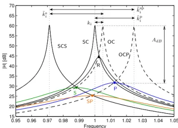
Figure 4.The FRFs(equation (26)) of a 1 dof EMS associated with

several resistive shunt circuits and several tunings of Rsh(te). SC and OC: short- and circuit response without a NC; OCP: open-circuit response with a negative capacitance in parallel configuration; SCS: short-circuit response with a negative capacitance in series configuration; R (R-shunt), P (parallel), S (series) and SP (series +parallel): response of the EMS with the optimal value of Rsh(te) for each NC layout.

2.7. Effect of negative capacitance

The MEMCF without any NC for mode i is ki, defined by

equation (12). When we consider a negative capacitance in

parallel or series configuration, we have defined an enhanced

coupling factor k˜ , which is the coupling factor of the EMSi

viewed from the shunt impedance Zsh, and thus including the

negative capacitance. Table 1 shows the values of k˜i (see

equation(23)), which are always higher than kiif the stability conditions of section2.6are fulfilled. The main effect of the

negative capacitance is to artificially4 increase the MEMCF

by changing the capacitance of the piezoelectric patch viewed

from the shunt (the equivalent capacitance for series and

parallel configurations, given by equations (20)). According

to Thomas et al[2], the higher the MEMCF is, the better the

vibration attenuation provided by the resistive shunt is. Thus, the addition of the NC allows the attenuation performance

provided by the shunt control to be artificially improved.

The increase in the MEMCF can also be viewed as an increase in the distance between the open- and short-circuit eigenfrequencies(see table1), as shown in figure4. As for the

parallel configuration, the short-circuit eigenfrequencies are

not changed by the presence of the NC, whereas the open-circuit eigenfrequencies are shifted towards higher frequency values. Note that the closer C1 is to the stability limit, the higher wioc and k˜ are. As for the series coni figuration, the

open-circuit eigenfrequencies are not changed by the presence of the NC, but the short-circuit eigenfrequencies are shifted

towards lower frequency values. The closer C2is to the

sta-bility limit, the lower wisc is and the higher k˜ is.i

The addition of the NC makes it possible to increase the MEMCF by shifting either the open- or short-circuit eigen-frequency, depending on the way the NC is connected to the piezoelectric patch and the resistance Rsh (i.e. in parallel or

series). The next section proposes a new shunt circuit layout

with a couple of NCs and a resistance. The use of two NCs together allows both the open- and short-circuit eigen-frequencies to be shifted at the same time. Thus, the increase in the MEMCF is higher than that achievable by using

par-allel and series configurations. A detailed comparison of the

enhancement of the MEMCF provided by the three con

fig-urations(i.e. series, parallel and the new one) will be given in the next section.

3. A new electrical circuit layout with negative capacitances

The previous sections showed that the use of an NC arti

fi-cially increases the MEMCF. The idea behind the new circuit proposed herein is to increase the open-circuit eigen-frequencies and to decrease the short-circuit eigeneigen-frequencies at the same time by using two NCs: one connected in parallel (-C1) and the other in series (-C2), as in evidence in figure5.

Therefore, this new configuration is named the

series+par-allel(SP) configuration.

3.1. Analytical model

Relying onfigure5and following the same approach used in

section2.4, equation(2b) is replaced by:

å

If this model is restricted to the ith vibration mode ( = " ¹q_n 0 n i), using the model proposed in equation (9)

with the static correction, one defines the following equivalent capacitance: = -+ -C C C C C C C . 32 i i eqsp p 1 2 1 2 p ( ) ( )

for the network made up by the three capacitances(Cpi, -C1

and -C2).

Then, using the change of variable of equation(21) with

=

Ceq Ceqsp, the model of equations (22a), (22b), (22c) is

obtained again with the following short- and open-circuit eigenfrequencies: w = w - c + -C C C 33 i i i i sc 2 2 1 2 p ( ) w = w + c -C C 34 i i i i oc 2 2 p 1 ( )

and with t = R Ce sh eqsp.

As expected, the use of two NCs in the shunt circuit allows us to decrease the short-circuit eigenfrequencies and to increase the open-circuit ones at the same time, thus leading to an enhanced MEMCF k˜: = - + -k k 1 1 35 i i C C C C C C i i 1 p 1 2 p 2

(

)

(

)

This is illustrated in figure4.

The analytical formulation of the FRF of the SP con

fig-uration described here is exactly the same as that of the series

and parallel configurations (and of the simple R-shunt, see

section 2.4 and [2]), defined by equation (26), where the

values of wisc, wiocand teto be considered depend on the NC

layout used. The parameters involved in the definition of Hi

Figure 5.The new proposed circuit with two NCs.

4 _{We say artificially because the MEMCF is an intrinsic property of the EMS}

that depends on the piezoelectric material and on the geometry of the system.

are gathered in table 1 for the parallel, series and SP configurations.

3.2. Stability conditions for the ideal SP configuration

The stability condition for SP can be deduced by those of

section2.6or, equivalently, by applying the Routh–Hurwitz

criterion to the denominator of equation (26). The most

restrictive conditions relating to the first and last modes (as

explained in section2.6) are:

< ¥ + >

C1 C and C1 C2 C0 (36) In this case we found two stability conditions to be

satisfied at the same time. Indeed, the open-circuit

eigen-frequency of the highest mode must not shift to +¥ and the

short-circuit eigenfrequency of thefirst mode must not reach

the null frequency. 3.3. Effect on the MEMCF

The new circuit proposed herein is able to increase the

MEMCF more than the series and parallel configurations, as

explained in the previous sections. A straightforward approach to having a quantitative understanding of the

ben-efits provided by the SP configuration is possible by

con-sidering a single-degree-of-freedom system. We define four

indexes able to describe how much the negative capacitance, related to each possible configuration, is far from Cpi: b1for

the parallel, b2 for the series, and bsp1 and bsp2 for the SP

configuration. Their expressions are:

b b b b = = = = + C C C C C C C C C , , , 37 i i i i 1 1 p 2 p 2 sp1 1 p sp2 p 1 2 ( )

With these definitions, null β values correspond to a situation

where no NCs are added to the circuit ( =C1 0 and

= +¥

C2 ). In contrast, β coefficients equal to one mean

that the values of the NCs are beyond but close to the instability condition.

Table 2 gathers the values of w_isc, w_ioc, k˜ and ti e as a

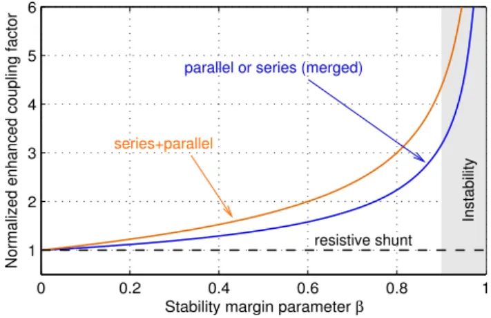
function ofβ, obtained with those of table1. Figure6shows

k k˜i i(i.e. normalised enhanced coupling factor) as a function

of β (achieved with the closed form expressions of the third

row of table 2) and enables the benefit of the negative

capacitance to be interpreted in terms of MEMCF

enhance-ment. The two single capacitance configurations (series and

parallel) give the same coupling factor enhancement for a

given value of theβ index. Moreover, for any value of β, the

SP configuration always displays higher k˜ values than ai

single negative capacitance in series or in parallel.

Since k˜ tends to +¥ wheni β approaches 1, one might

think it possible to design a negative capacitance circuit with

infinite performance. However, the performances are limited

by the stability limit(see equations (36), (30) and (29)), which

are discussed here as a function of theβ indexes. The value of

β, defined above, depends on Cpi and thus only on the ith

mode considered in the corresponding 1 dof model. Actually,

the value(s) of β for which the system becomes unstable

depend on C0andC¥ (see sections2.6and3.2):

b =b = C¥ b =b = C C C , , 38 i i 1 inst sp1 inst p 2 inst sp2 inst p 0 ( )

and thus depend on the complete N dof model and not only on

the considered ith mode, as Cpi does. In practice,

> > ¥

C0 Cpi C , depending on the considered mode, so that

the stability limits in terms ofβ are smaller but close to one. We can notice fromfigure2that the binst_{coefficients for the}

series and parallel cases are different. Moreover, the closer Cpiis to C∞(parallel) or C0(series), the higher the stability threshold on the value ofβ is (i.e. the higher the value of binst

is) and the the higher the attenuation performance is. Hence,

the maximum achievable value of β for the two NC

configurations depends on the mode considered. Two extreme

cases are worth taking into account:

• according to equation (16), if the considered mode is in

the low frequencies of the EMS spectrum, Cpi will be

closer to C0than toC¥, so that the stability limit for the series configuration ( >C2 C0Cpi) will be reached for

values of b2 close to 1 (b2  1

inst _{), whereas the stability}

limit for the parallel configuration ( <C1 C¥<Cpi) will

be reached for values of b1 far from 1 (b1inst< 1).

According tofigure6, in this case the series configuration will perform better than the parallel configuration; • the opposite situation holds for high-frequency modes:

the parallel configuration will theoretically perform better than the series one (b₁inst 1,b₂inst< 1).

To fix the ideas, we present an example considering an

arbitrary EMS with 10 degrees of freedom. This example will allow us to explain clearly when it is convenient to use either

the parallel or the series configuration, and when the SP

becomes highly efficient if compared to these traditional NC

layouts. In the example, the modes of the EMS are assumed to

have the same MEMCF value, which is ki= 0.1. The values

Figure 6.The trend of the EMEMCF k˜ , normalised by ki i(k k˜i i), as a

function ofβ, for the three NC configurations (parallel, series and series+parallel), with b=bp=bs=bsp1=bsp2. The grey region

shows an example of the region for which the system is unstable, for β above 0.9 in this particular case.

of Cpi(equation (14)), as compared to C0(equation (15)) and

¥

C , are gathered in table3for thefirst, the fifth and the ninth

mode. As for the first mode, the series configuration works

better than the parallel one at the stability limit because the first mode is in the low frequency part of the spectrum.

Indeed, the series configuration is able to increase the

coupling factor by a factor of 10, whereas the parallel one allows us to achieve a value of EMEMCF just 3.56 times the original MEMCF. As for the ninth mode, located in the upper part of the frequency spectrum, the opposite result is

observed. As for the fifth mode, the parallel and series

configurations show the same performance: a coupling factor

enhancement of a factor 4.47 is achieved by both the NC

configurations. The performance of the SP configuration is

also shown in table 3. Since its stability depends on two

conditions, related to the two negative capacitances in series

and in parallel, the best gain in using an SP configuration as

compared to a single NC in parallel or series configuration is

for the medium frequency modes: for mode 5, the SP

configuration gives a coupling factor enhancement of 6.24

times instead of 4.47 (obtained with the traditional NC

layouts).

4. Optimisation and performance with ideal circuits

Sections 2 and 3 described the mathematical model to treat

EMSs shunted with impedances made up by NCs and Rsh as

well as the effect of NCs on the MEMCF. This section is aimed at the derivation of the analytical procedures for

defining the optimal values of the shunt impedance

compo-nents(i.e. NC and Rsh) in order to achieve the best vibration

reduction, as well as for the quantification of the performance of the shunt in terms of vibration reduction.

4.1. Tuning of the negative capacitance

Section 3.3showed that the closer the negative capacitances

are to the stability limits, the higher the EMEMCF is. Therefore, the attenuation performance can be improved using negative capacitances as close as possible to the stabi-lity limits.

4.2. Tuning of the resistance Rshfor single mode control The other component of the shunt circuit to be tuned is the resistance Rsh. This section explains how to optimise it when

single mode vibration reduction is required. The criterion proposed herein is based on considerations of the shape of the controlled FRF of the EMS.

If the mechanical system to damp shows low modal density, we can approximate the response of the EMS as the

one given by the ith mode. Therefore, it is possible to define

the optimal value of Rsh by considering the FRF Hi of

equation(26), which is valid for the R-shunt without the NC

[2] as well as for the parallel, series and SP configuration, in

the case of a 1 dof approximation of the model (see

section 2.5). This means that the procedure used to find the

optimal value of Rsh for a traditional R-shunt can be applied

to the present cases with the negative capacitance. It will also provide results of the same form for the three layouts.

As suggested in[1,2,18,19], the optimisation problem

is solved by neglecting the structural dampingx_i. Under such

a hypothesis, there exists a point (here denoted by F )

com-mon to the amplitudes of all the FRFs of the EMS when Rshis

varied. Since F is common to all curves describing the

Table 2.Parameters of the EMS enhanced by NCs in parallel, series or series+parallel configurations, as a function of the stability margin

parameterβ.

R-shunt Parallel config. Series config. SP config.

SC freq. w_isc _w i wi w - b b -1 i k 1 i 2 2 2 w -b b -1 i k 1 i sp2 2 sp2 OC freq. wioc wˆi=wi 1+ ki2 w + b -1 i k 1 i2 1 wˆi=wi 1+ ki2 w + b -1 i k 1 i2 sp1 EMEMCF k˜i ki _-b k 1 i 1 -b k 1 i 2 b b b b - -ki 1 sp1 1 sp2 1 sp1 sp2 ( )( )

Elec. time const. te R Csh pi R Csh pi(1-b1) _-b R C 1 i sh p 2 b b b b - -R C 1 1 1 i sh p sp1 sp1 sp2 sp2 ( )( )

Table 3.Value of Cpiand stability limits in term of theβ indexes and corresponding coupling factor enhancement k k˜i ifor an arbitrary EMS

with ten natural modes, with ki= 0.1 for all the ten modes.

Parallel config. Series config. SP config.

Cpi C0 Cpi C¥ b1inst k k˜i i b2inst k k˜i i k k˜i i

mode 1 1/1.01 1.09 0.92 3.56 0.99 10 10.56

mode 5 1/1.05 1.05 0.95 4.47 0.95 4.47 6.24

amplitude of the FRF, the optimum one (the one which has

the lowest peak amplitude) is that with its maximum at point

F. The frequency value wF associated with point F can be

obtained by remarking that, among all possible FRFs, this point is common to two particular cases: the one in the short-circuit (Rsh=0 and t =e 0) and the one in the open-circuit

(Rsh= +¥ and t = +¥e ), for which the FRF expression

assumes a simple mathematical form. The frequency wF is

found to be: w = w + w 2 39 F i i oc 2 sc 2 ( ) ( ) ( )

where w_ioc and w_isc are calculated depending on the

configuration used (i.e. series, parallel, SP; see table1). The

associated optimal value for teis:

t w = 1 40 e F opt ( )

The above reasoning is illustrated in figure 4, where the

location of point F is shown with a bullet on the R, S, P and

SP optimised curves(with te=teopt), depending on the NC

configuration considered. The above theoretical results are

also validated since these optimised responses have their

maximum at the crossing of the corresponding OC (i.e.

= +¥

Rsh ) and SC (i.e.Rsh=0) curves.

The above parameters t_eopt and wF can be rewritten in

terms of k˜i by noticing that woc 2i =wi2ki + wi

2 _{sc 2}

( ) ˜ ( )

(equation (23)) and by writing w( isc 2) =wi2(1 - K2), with K defined in table4. One obtains:

w t w = 1 = k + -2 2K 2 . 41 F e i i opt 2 ₂ ˜ ( )

Finally, the optimal value of Rshcan be obtained by using the

above equation together with the last row of tables1or 2.

4.3. Performance evaluation for single mode control

The performance of the shunts is evaluated by defining the

vibration attenuation parameter AdB, proposed in[2,20] for

passive shunts, as: = A H H 20 log 42 dB 10 sc sh ( )

where Hsc is the FRF peak amplitude in short-circuit

configuration without any shunt (i.e. uncontrolled EMS) and

= W=w t t=

Hsh ∣ ∣Hi F,e eopt is the FRF peak amplitude with the

optimised shunt(with te=teopt) connected. AdB is shown in figure 7. Since Hsc=1 2x wi i 1-xi

2 2

( ), after some

sym-bolic manipulations, one obtains a single expression of AdB

valid for all four shunt layouts studied in this paper:

x x x = + + -A 20 log k 2 2 2 k 2K 4 1 43 i i i i i dB 10 2 2 ₂ 2 ˜ ˜ ( )

where the enhanced coupling factor k˜ takes the values of thei

third rows of tables 1and 2 depending on the configuration

used. The values of K are gathered in table4.

The first major result from equation (43) is that, for a

negative capacitance shunt in parallel configuration, AdBhas

the same form as the one for a standard R-shunt, provided kiis replaced by the enhanced coupling factor k˜ . As for the seriesi

and SP configuration, a slight difference is brought about by

the term K2. In these two latter situations, by noticing

(tables2 and4) that K and k˜ are functions of ki iandβ only,

AdBcan be expressed as a function of k˜ and bi 2(or bsp2) only.

To evaluate the effect of K2,figure7shows AdBas a function

of k˜ for several values of xi i. It shows that, for each value of xi,

all the curves are almost merged, so that in practice the effect

of the term K2can be neglected: for a negative capacitance

shunt, AdB has the same form as the one for a standard

R-shunt, provided ki is replaced by the enhanced coupling

factor k˜ . This result is very interesting in practice since iti

enables us to estimate the performance of the negative shunts relying only on two simple graphs. Indeed, it is sufficient:

• to know the values of the MEMCF ki and the damping

factor x_ifor the considered mode;

• to know the margin from the stability limit of the

considered negative capacitance shunt(the value of β, see

section 3.3). Then, figure 6 enables us to estimate the

increase in the coupling factor, from kito k˜i;

• then, figure 7 leads us to estimate the resonance

attenuation brought about by the considered shunt as a function of k˜ and xi i.

In the same manner as for a standard R-shunt (see [2]), the

higher the coupling factor ki is and the lower the structural

damping x_i is, the better the attenuation performances are. Another way of evaluating the shunt performances is to

consider the magnification factor at resonance D—that is the

ratio between the resonance peak amplitude Hshand the static

(for W = 0) amplitude of the FRF (Hi(W = 0)=1 (wisc 2) ).

Figure8shows D as a function of k˜ . An interesting point isi

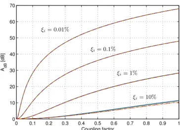
Figure 7.Attenuation AdBachievable with the four shunt layouts as a

function of the coupling factor ki(for the R-shunt) and of the enhanced coupling factor k˜ for the shunts with NCi (parallel, series and SP), for several values of structural damping xi. For each value of xi, four curves are merged, one for each configuration: parallel, series, SP and simple resistive shunt.

that for low structural damping x_iand a high coupling factor, several D curves are merged, so that D only slightly depends on x_i(for instance, the curves for x = 0.1%_i and x = 0.01%_i are merged fork˜i>0.2). As a consequence, with large cou-pling factors achievable using NCs, the amplitude at reso-nance depends mainly on the coupling factor and no longer on the damping factor.

4.4. Tuning of the resistance Rsh and performance evaluation for multi-mode control

When multi-mode control is required, numerical minimisa-tions can be carried out in order tofind the value of Rshwhich

fulfills the desired goal (e.g. H_∞ control, H2control). This

section explains how tofind the value of Rshwithout carrying

out any numerical minimisation and thus avoiding any

pos-sible problems relating to minimisation procedures(e.g. local

minima). This goal will be achieved by means of an

easy-to-apply graphical approach relying on an analytical formula-tion, as explained underneath.

For a given value of Rsh (and thus of te), we call wir the

resonance frequency of mode i, i.e. the frequency for which

the FRF modulus H∣ ∣ reaches its maximum. We havei

w_isc<w_ir<w_ioc _{when t}

e is varied. This resonance frequency

wir can be calculated by solving the following equation as a

function ofΩ: ¶ W ¶W = H 0 44 i 2 ∣ ( )∣ ( )

Once w t wir(e, i) is known as a function of te, the amplitude at

the resonance can be derived with equation (26):

w

= W =

Hi Hi i . 45

max r

∣ ( )∣ ( )

It must be noted that the performance indicator AdB

(equation (42)) is related to the value of H_imax for te=te opt

since Hsh=Himax∣t te= eopt.

To calculate wir, equation (44) gives (if xi is considered

null, as done when calculating wF) the following seventh

order equation inΩ: W W + W + W +₍a 6 b 4 c 2 d₎=0 ₍46₎ where t t w t w t w t w t w = = -= - = - -a b c d 2 , 4 2 , 2 4 , 2 47 e e i e i e i e i e i 4 2 oc 2 4 oc 2 2 oc 4 2 sc 4 2 sc 2 ( ) ( ) ( ) ( ) ( ) ( )

The terms w_isc and w_ioc must be calculated according to the configuration used (see table1).

Equation(46) leads to the trivial solution W = 0 and to

three other possible solutions for W2_{. The third order equation}

in W2 _{can be solved analytically by using the formula found}

by Tartaglia[21]. Let us define:

= - = -+ D = + p c a b a m d a bc a b a m p 3 , 3 2 27 , 4 27 48 2 2 2 3 3 2 3 ( ) ( ) ( ) ( )

If D < 0, the solutions of the cubic equation in W2 _(see

equation46) are: J W =1 2 -p 3 cos 3 -b 3a 49a 2 [ ] ( ) ( ) J p W =22 2 -p 3 cos[( +2 ) 3]-b (3a) (49b) J p W =3 2 -p 3 cos +4 3 -b 3a 49c 2 [( ) ] ( ) ( )

where J =arctan[ -D -m( 2)] and arctan must be

intended as the four-quadrant arctangent. If D0, the

solutions are not provided here because when Δ is higher

than or equal to zero, the attenuation provided by the shunt is usually so high that the resonance is canceled by the control action. As a result, the maximum of H∣ ∣ between wi i

sc_{and w} i oc

is lower than its static component (i.e.

w

W = =

Hi 0 1 isc 2

∣ ( )∣ ( ) ), and the only physical solution

provided by equation (46) is w = 0ir 5. Therefore, if the

Table 4.Definition of K.

R-shunt Parallel Series SP

K= 0 K= 0 K=_w c_- =k _-b_b C C i 1 i i 2 pi 2 2 K= = c w b b + - k -C C C i 1 i i 1 2 pi sp2 sp2

Figure 8.The magnification factor at resonance D due to the four

shunt layouts as a function of the coupling factor ki(for the R-shunt) and of the enhanced coupling factor k˜ for the shunts with NCi (parallel, series and SP), for several values of structural damping xi. For each value of xi, four curves are merged, one for each configuration: parallel, series, SP and simple resistive shunt.

5

This result was checked by means of simulations with

/ /

p <w < p

2 10 rad s i 2 3000 rad s, 0.001<ki<0.3, 0<b<1 and

teopt 100<te<100teopt. We chose the simulation values in order to cover

chosen value of tegives a value ofΔ higher than or equal to

zero, the maximum of the amplitude of Hi can be

approximated by its static component. If the chosen value

of tegives a value ofΔ lower than zero, the three solutions

(49a)–(c) must be taken into consideration. Only one of them

has a physical meaning and it is found to be (49a).5 If a

different situation with respect to the cases considered in footnote 5 is taken into account, and equation(49a) does not

provide a physical solution, solutions(49b) and (49c) must be

considered, because one of them will provide the correct one. Therefore, the curves relating the value of Rsh to Himax

can be drawn for all the modes to be controlled. This gives us

the possibility offinding out the optimal value of Rsh for a

given control problem with a graphical approach, as explained in the following example. Let us consider the

system described in table 5 (similar to that used for

exper-imental tests in the following), an NC in series and a H_∞

control problem on the velocity of a given point of the EMS. If xmis a point where the structural response is measured and

xf is a point where an excitation force is provided, the FRF

between this force and the displacement of the structure in xm is obtained by multiplying equation (26) by Fi(xm)Fi( ).xf

Hence, for each of the modes considered it is possible to draw

the curve relating Rsh to the maximum of the velocity FRF:

w

= F F

vimax ∣ i( )xf i(xm) irHimax∣ (50)

The resulting curves are plotted infigure9. In thisfigure, the

graph has te on the x-axis in place of Rsh because Cpi was

fixed to the same value for all four modes (indeed the values

of Cp1 to Cp4 were so close that an average value has been

used) and thus a given value of Rsh corresponds to the same

value of tefor all the modes. The portions of the solid curves

with an increased width (blue and orange in figure 9) are

those providing evidence of the highest peak of the velocity

FRF for the EMS as a function of te. The minimum of this

line corresponds to the value of Rsh to be chosen if an H¥

control must be performed. This figure clearly shows the

optimal value of te without the need to carry out numerical

minimisations, and evidence of this optimal value is provided

by a star in thefigure. The same procedure can be applied to

acceleration as well, just by multiplying equation(50) by w_ir.

This graphical approach can also lead us to find the

optimal value of Rsh for other control problems. As an

example, for an H2 control in velocity(i.e. minimisation of

the velocity root mean square value, RMS), one can consider

minimising the following approximated quantity:

å

The minimum of this curve (solid green curve in figure 9),

highlighted by a triangle infigure9, shows which value of te

makes the RMS minimum. Note that the H_∞ control (star)

and the H2control(triangle) require different solutions, which

can easily be found graphically, and the optimal values of te

for the H2and H∞problems do not correspond to the optimal

values of the four modes (minima of the solid thin lines of

figure9).

This graphical approach works with FRFs, but it even allows us to solve problems where the input disturbance is not

white random noise. Indeed, if the power-spectrum Gddof the

disturbance can be estimated, the control problem can be expressed not in terms of FRF but in terms of power-spectrum

of the EMS response Grr, which can be calculated in case of

low modal density as:

w = w F F w

Grr i Gdd i i xm i x Hf i i 52

r r r 2

( ) ( )∣ ( ) ( ) ( )∣ ( )

5. Real circuits

5.1. Negative capacitance layouts

Section1mentioned that an NC can be built using OP-AMPs

and that we distinguish two different types: ideal circuits (ICs), which can be modelled as pure NCs, and more

com-plicated circuits (real circuits, RCs), which cannot be

modelled as pure negative capacitances. RCs are often used in

practice because they offer significant advantages when

compared to ICs. Indeed, they are able to overcome some of the main issues relating to ICs. All the circuits are discussed in this section.

A negative impedance can be built in practice by using an OP-AMP along with three different impedances

Figure 9.The trend of vi

max

and ARMSfor the four modes of the EMS described in table5for an NC in series configuration. Cpi= 30.5 nF and C2= 36.6 nF. The values of the mode shape components used here are: F( )xf =[1.7167, 0.2450, 0.8020, 1.1987] and¢

F(xm)=[2.3452, 2.2935,-2.8761,-2.2822] .¢

Table 5.Modal data of the system used for the numerical simulations

and for the experimental tests.

Mode number wi (2p)[Hz] xi ki

1 39.72 0.0045 0.2716

2 187.34 0.0030 0.1037

3 509.00 0.0026 0.0710

(i.e. Z1, Z2, Z3), as shown in figure10. The impedance of this

circuit(the ratio between voltage and current intensity V I)

is: = -Z Z Z Z 53 nc 1 3 2 ( )

Equation(53) is valid as long as the OP-AMP is considered

ideal, which in turn means that the voltage difference between the inputs is null and no currentflows in the inputs [15]. Znc

becomes an NC if Z1, Z2and Z3are replaced by resistances

and a capacitance respectively. In order to obtain a pure

negative capacitance—as in figure 3(c)—two different

configurations are possible, labelled type A and type B

circuits, as shown infigures11(a), (b). In this case, we have

an equivalent negative capacitance -Cn with:

= C R C R 54 n 2 1 ˆ ( )

and the corresponding circuits are denoted as ideal

circuits(ICs).

Furthermore, some authors suggest adding a resistance Rˆ in parallel to the capacitance Cˆ [22], leading to the circuits of

figures11(c) and (d) (types AR and BR). These circuits, denoted

as real circuits(RCs) in the following, are not pure NCs: their

impedance Znc is equivalent to a pure NC, - Cn, (see

equation(54)) in parallel with a negative resistance, -R,˜ with:

= R R R R 55 1 2 ˜ ˆ _{( )}

The parallel between Cˆ and Rˆ constitutes an undesired but

necessary high-pass filter useful for solving practical

problems such as bias-current and offset-voltage induced errors[22].

The addition of Rˆ is often necessary when a series con-figuration is taken into consideration. Instead, in the parallel

configuration, the parallel between the capacitance of the

piezoelectric actuator and Rsh (see section 5.2) already

con-stitutes a high-passfilter. Nonetheless, the addition of Rˆ can

be useful even in this case (as found in the experiments

related to this paper) because the values of the capacitance of

the piezoelectric actuator and Rsh can be unsuitable for

properly stopping the low-frequency components. In such cases, it is useful to add Rˆ in order to produce a further

parallel between Cˆ and Rˆ and thus a more efficient high-pass

filter. Moreover, the polarity of the OP-AMP is of practical

importance (it has no influence in theory since equation (53)

is the same whatever the + - input pin wiring be). As for a

parallel configuration, the circuits of figure11 can be used.

For a series connection, the OP-AMP + - input pins must be inverted. Most of the circuits presented here and used to build an NC are employed in the literature, without providing any

comparison between the different solutions. Table 6 shows

how different authors have used different layouts.

The theoretical analyses carried out so far, in sections2, 3and 4, regard ICs without Rˆ. The effect of adding Rˆ to the circuit on the behaviour of the shunt is now addressed. 5.2. Parallel configuration for real circuits

An RC in parallel configuration can be modelled as shown in

figure 12(a). The total resistance in parallel to the

piezo-electric actuator is the parallel between Rshand -R˜(due to the

presence of Rˆ, see equation(55)), which is named Rp:

= -R RR R R 56 p sh sh ˜ ˜ ( )

This total resistance Rp can be considered as the new shunt

resistance, and thus the analytical treatment is the same as the

ICs in a parallel configuration with just one difference: the

resistance Rsh must be replaced by Rp in the equations of

sections 2, 3 and 4. Hence, the RCs in the parallel

configuration can be fully described by the model presented

so far. Therefore, the stability of the EMS is guaranteed if the

condition of equation (29) is fulfilled and Rp0, and the

tuning and performance of the shunt are those predicted in section4.

5.3. Series configuration for real circuits

An RC in a series configuration can be modelled as shown in

figure12(b). The impedance Zrsof the circuit composed by

-C2, -R˜ and Rsh in the Fourier domain is:

= -+ W Z R R j RC 1 57 rs sh 2 ˜ ˜ ( )

where the values of C2and R˜ depend upon the values of R1,

R2, Cˆ and Rˆ (see equations (54) and (55)). Generally

speaking, this circuit cannot be treated with the formalism

of sections 2, 3.3 and 4. Nevertheless, there are some cases

where the effect of R˜ can be neglected, depending on the

frequency band of interest, as shown in sections 5.3.1

and 5.3.2.

5.3.1. Similar behaviour of RCs and ICs. If Rˆ—and thus R˜—

tend to +¥, the impedance Zrs tends to that of an IC that

writes: = -W Z R j C 1 58 is sh 2 ( )

In the high frequency range W 1 ( ˜RC2), the effect of Rˆ can

be neglected sinceZrsZis(see figure13) and the behaviour

of the real circuit is the one of a pure negative capacitance(in series with Rsh). As a consequence, if all the controlled modes

Figure 10.A negative impedance built by means of an OP-AMP(a)

of the EMS have their natural frequency above1 ( ˜RC2), it is

possible to use the results of sections 2, 3.3 and 4 without

paying attention to Rˆ.

It is possible to use the analytical formulation derived for ICs in a further case, even if the frequency range considered is below1 ( ˜RC2). This is the case in which the value chosen for

Rshis high. In this case the values of teopt, wirand AdBobtained

with Zrsand Zisare usually very close. Such similar results for

Zrs and Zis are shown in section 6.2 (see figure 17 in

particular). The different behaviour between Zrs and Zis

becomes evident when Rshis low, and in this case significant

differences in the attenuation performance on the modes at low frequency become clear. Again, such a fact is shown in section6.2. It is noticed that low values of Rsh mean that the

control action is focused on the modes at high frequency.

5.3.2. Use of a compensation resistance. If the EMS shows natural frequencies to be controlled at low frequencies, below

RC

1 ( ˜ 2), and if the value of Rsh we use is low, the analytical

treatment used for ICs is not reliable for RCs. The IC and RC series circuits only differ for the presence of -R˜, which degrades the shunt performances. The effect of -R˜ can be cancelled by adding a further passive resistance Rsin parallel

to -R˜ and -C2, as shown in figure 12(c). The parallel

between Rsand -R˜ (which is physically obtained by placing

Rs between the upper connector of the impedances in

figures 11(c), (d) and the ground) gives an equivalent

resistance Req, defined as:

= -R RR R R 59 eq s s ˜ ˜ ( )

The aim is to achieve high negative values of Reqin order to

cancel out the effect of R˜. Consequently, the required values

of Rs should be close to R˜ ( Rs R˜), which produce high

negative values of Req(∣Req∣ +¥) and thus cancel out the

effect of Rˆ. In such a case, all the results of sections2, 3.3and

4are valid and it is not necessary to consider Rˆ. If the use of

the compensation resistance Rs must be avoided for any

practical reason (see section6.2), a new analytical treatment

can be developed for the shunt circuit in figure 12(b) (i.e.

composed of -C2, -R˜ and Rsh). This analytical treatment is

given in appendixA.

5.4. SP configuration for real circuits

The SP circuit has been treated in section3and it is possible

to deduce that this new configuration can be seen as an NC in

Figure 11.Practical circuits to build a negative capacitance: type A(a), type B (b), type AR (c) and type BR (d) circuits in parallel

configuration. For the series configuration, the pins of the OP-AMP must be exchanged.

Table 6.The NC layouts used in the literature, defined in figure11.

All series configurations have the OP-AMP + - input pins exchanged with respect tofigure11.

Authors Parallel configuration Series configuration

Behrens et al[4] - Type AR

Park and Baz[6] Type B

-de Marneffe and Preumont[3] Type B Type B Manzoni et al[7] - Type AR Kodejska et al[8] - Type BR Beck et al[9,10] - Type BR

This paper Type B(A, AR, BR