HAL Id: hal-01111981
https://hal.archives-ouvertes.fr/hal-01111981v2
Submitted on 17 Jul 2015
HAL is a multi-disciplinary open access
archive for the deposit and dissemination of
sci-entific research documents, whether they are
pub-lished or not. The documents may come from
teaching and research institutions in France or
abroad, or from public or private research centers.
L’archive ouverte pluridisciplinaire HAL, est
destinée au dépôt et à la diffusion de documents
scientifiques de niveau recherche, publiés ou non,
émanant des établissements d’enseignement et de
recherche français ou étrangers, des laboratoires
publics ou privés.
Maxime Lenormand, Bruno Goncalves, Antònia Tugores, José Javier Ramasco
To cite this version:
Maxime Lenormand, Bruno Goncalves, Antònia Tugores, José Javier Ramasco. Human diffusion
and city influence. Journal of the Royal Society Interface, the Royal Society, 2015, 12, pp.20150473.
�10.1098/rsif.2015.0473�. �hal-01111981v2�
Maxime Lenormand,1 Bruno Gon¸calves,2 Ant`onia Tugores,1 and Jos´e J. Ramasco1
1
Instituto de F´ısica Interdisciplinar y Sistemas Complejos IFISC (CSIC-UIB), 07122 Palma de Mallorca, Spain
2Aix Marseille Universit´e, Universit´e de Toulon,
CNRS, CPT, UMR 7332, 13288 Marseille, France
Cities are characterized by concentrating population, economic activity and services. However, not all cities are equal and a natural hierarchy at local, regional or global scales spontaneously emerges. In this work, we introduce a method to quantify city influence using geolocated tweets to characterize human mobility. Rome and Paris appear consistently as the cities attracting most diverse visitors. The ratio between locals and non-local visitors turns out to be fundamental for a city to truly be global. Focusing only on urban residents’ mobility flows, a city to city network can be constructed. This network allows us to analyze centrality measures at different scales. New York and London play a predominant role at the global scale, while urban rankings suffer substantial changes if the focus is set at a regional level.
Ever since Christaller proposed the central place theory in the 30’s [1], researchers have worked to un-derstand the relations and competition between cities leading to the emergence of a hierarchy. Christaller envisioned an exclusive area surrounding each city at a regional scale to which it provided services such as markets, hospitals, schools, universities, etc. The ser-vices display different level of specialization, induc-ing thus a hierarchy among urban areas accordinduc-ing to the type of services offered. In addition, this idea naturally brings an equidistant distribution of urban centers of similar category as long as no geographical constraints prevents it. Still, in the present global-ized world relations between cities go much beyond mere geographical distance. In order to take into ac-count this fact, it was necessary to introduce the con-cept of world city [2]. These are cities that concen-trate economic warehouses like the headquarters of large multinational companies or global financial dis-tricts, of knowledge and innovation as the cutting edge technological firms or universities, or political decision centers, and that play an eminent role of dominance over smaller, more local, counterparts. The concept of global city is, nevertheless, vague and in need of fur-ther mathematical formalization. This is attained by means of so-called world city networks, in which each pair of cities is linked whether they share a common resource or interchange goods or people [3–7]. For in-stance, a link can be established if two cities share headquarters of the same company [7–9], if both are part of good production chains [10], interchange fi-nance services [11], internet data [12] or if direct flights or boats connect them [4,13–15]. Centrality measures are then applied to the network and a ranking of the cities naturally emerges. Due in great part to their geographical locations and traditional roles as trans-Atlantic bridges, New York and London are typically the top rankers in many of these studies [5, 9, 14]. There are, however, inconsistencies in terms of the meaning and stability of the results obtained from dif-ferent networks or with difdif-ferent centrality measures [14, 16] and a more organic and stable definition is needed.
Here we use information and communication
tech-nologies (ICT) to approach the problem from a differ-ent perspective. How long would information originat-ing from a given city require to reach any other city if were to pass from person to person only through face to face conversations? Or, in other words, what is the likelihood that that information reaches a certain dis-tance away after a given time period. In this thought experiment, the most central place in the world would simply be the one where the message can reach ev-erywhere else in the shortest amount of time. This view allows us to easily define a temporal network of influence.
We perform this analysis by empirically observing how people travel worldwide and using that as a proxy for how quickly our message would be able to spread. The recent popularization and affordability of geolo-cated ICT services and devices such as mobile phones, credit or transport cards gets registered generating a large quantity of real time data on how people move [17–25]. This information has been used to study questions such as interactions in social networks [26–
29], information propagation [30], city structure and land use [23,31–40], or even road and long range train traffic [41]. It is bringing a new era in the so-called Sci-ence of Cities by providing a ground for a systematic comparison of the structure of urban areas of different sizes or in different countries [37,38,40,42–47]. Data coming from credit cards and mobile phones are usu-ally constrained to a limited geographical area such as a city or a country, while those coming from on-line social media as Twitter, Flickr or Foursquare can refer to the whole globe. This is the reason why we focus here on geolocated tweets, which have already proven to be an useful tool to analyze mobility be-tween countries [48] and provide the ideal framework for our analysis.
In particular, we select 58 out of the most populated cities of the world and analyze their influence in terms of the average radius traveled and the area covered by Twitter users visiting each of them as a function of time. Differences in the mobility for local residents and external visitors are taken into account, in such a way that cities can be ranked according to the exten-sion covered by the diffuexten-sion of visitors and residents,
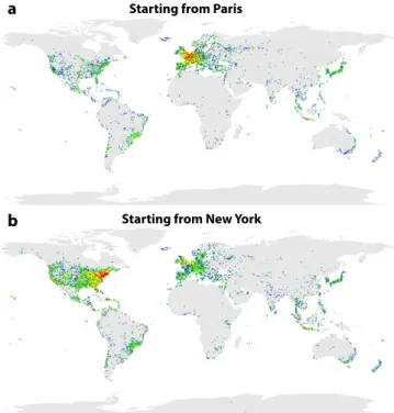
Figure 1: Positions of the geolocated tweets. Each tweet is represented as a point on the map location from which it was posted.
taken both together and separately, and by the at-tractiveness they exhibit towards visitors. Finally, we also consider the interaction between cities, forming a network that provide a framework to study urban communities and the role cities play within their own community (regional) versus a global perspective.
MATERIALS AND METHODS Twitter Dataset
Our database contains 21, 017, 892 tweets geolo-cated worldwide written by 571, 893 users in the tem-poral period ranging from October 2010 to June 2013 (1000 days). There are on average 36 tweets per user. Non-human behaviors or collective accounts have been excluded from the data by filtering out users travel-ing faster than a plane (750 km/h). For this, we have computed the distance and the time spent between two successive geolocated tweets posted by the same user. The geographical distribution of tweets is plot-ted in Figure1. The distribution matches population density in many countries, although it is important to note that some areas are under-represented as, for example, most of Africa and China.
We take as reference 58 cities around the world (see Table S1 in Appendix for a detailed account) that are both highly populated (most are among the 100 most populated cities in the world) and have a sufficiently large number of geolocated Twitter users. To avoid distortions imposed by different spatial scales and ur-ban area definitions that can be problematic [49,50], we operationally defined each city to be a circle of radius 50 km around the respective City Hall.
In order to assess the influence of a city, we need to characterize how users travel after visiting it. To do so, we consider the tweets posted by user υ ∆t
days after visiting city c. In Figure2, the locations of geolocated tweets are plotted according to the number of days since the first visit in Paris and New York as an example. Not surprisingly, a large part of the tweets are concentrated around these cities but one can observe how users eventually diffuse worldwide.
Starting from Paris
Starting from New York
a
b
Figure 2: Geolocated tweets of users who have been at least once in Paris (a) and New York (b). The color changes according to the number of days ∆t
since the first passage in the city. In red, one day; In yel-low, between 1 and 10 days; In green, between 10 and 100 days; And in blue, more than 100 days.
Definition of the user’s place of residence
To identify the Twitter users’ place of residence, we start by discretizing the space. To do so, we divide the world using a grid composed of 100 × 100 square kilometers cell in a cylindrical equal-area projection. In total there are approximately 5, 000 inhabited cells in our dataset. The place of residence of a user is a priori given by the cell from which he or she has posted most of his/her tweets. However, to avoid selecting users who did not show enough regularity, we consider only those users who posted at least one third of their tweets form the place of residence (representing more than 95% of the overall users). For each city, the number of valid users as well as the number of tweets posted from their first passage in the city are provided in Table S1 in Appendix.
We can now determine for each city if a user is res-ident (local user) or a visitor (non-local user). To do so, we compute the average position of the tweets posted from his/her cell of residence. If this position falls within the city boundaries (circle of radius 50 km around the City Hall) the user is considered as a local and as a non-local user otherwise.
∆
t(days)
R
(
km
)
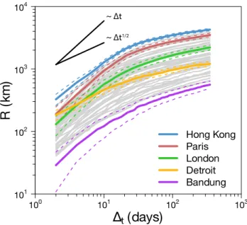
100 101 102 103 101 102 103 104 Hong Kong Paris London Detroit Bandung ~ Δt1/2 ~ ΔtFigure 3: Evolution of the average radius. Each
curve represents the evolution of the average radius R av-eraged over 100 independent extractions of a set of u = 300 users as a function of the number of days ∆tsince the first
passage in the city. In order to show the general trend, each gray curve corresponds to a city. The evolution of the radius for several cities is highlighted, such as the top and bottom rankers or representatives of the two main de-tected behaviors. Curves with a linear and square root growth are also shown as a guide to the eye. The dashed lines represent the standard deviation.
Metrics to assess city influence
We select a fixed number of users u in each city at random and track their displacements in a given pe-riod of time ∆t since their first tweet from it. Since
the results might depend on the specific set of users chosen, we average over 100 independent user extrac-tions. As shown in Figure S2 in Appendix, the longer ∆tis, the lower is the population of users who remain
active, so we must establish a tradeoff between num-ber of users and activity time. Unless otherwise stated we set u = 300 and ∆t = 350 days in the discussion
that follows.
Average radius
There are different aspects to take into account when trying to define how to properly measure the influence of a city due to Human Mobility. We start our discussion by considering the average radius trav-eled by Twitter users since their first tweet from a city c. We tracked for each user the positions from which he or she tweeted after visiting c, and compute the av-erage distance from these locations to the center of c. The average radius, R, is then defined as the average over all the u users of their individual radii.
The average radius is informative but can be biased
by the geography. Cities that are in relatively isolated positions such as islands may have a high average ra-dius just because a long trip is the only option to travel to them. To avoid this effect, we define the normal-ized average radius ˜R of a city c as the ratio between R (c) and the average distance of all the Twitter users’ places of residence to c (Figure S4 in Appendix).
Coverage
One possible way to overcome the limitation of the average ratio defined above is to discard geographic coherence all together and simply measure the geo-graphical area covered by those users, regardless of the distance at which it might be located from the originating city. In order to estimate the area cover by the users, the world surface has been divided in cells of 100 × 100 square kilometers as we have done to identify the users’ place of residence. By tracking the movements of the set of users passing through each city, we count the number of cells from which at least a tweet has been posted and define coverage as this number. This metric has the clear advantage of not being sensitive to isolated locations but it still does not consider how specific cells, specially the ones cor-responding to other important cities, are visited much more often than others.
RESULTS
Comparing the influence of cities
We start by taking the perspective from the city to the world and compare how effective the cities are as starting points for the Twitter users’ diffusion. The evolution of the average radius as a function of the time is plotted in Figure3for the 58 cities. The curves of the log-log plot show an initial fast increase followed by a much slower growth after approximately 15 − 20 days. The presence of these two regimes is mainly due to the presence of non-local users as it can be observed in Figure S5 in Appendix. In the initial phase, the ra-dius grows for all the cities at a rhythm faster than the square root of time, which is the classical predic-tion for 2D Wiener diffusion [51]. This is not fully surprising since the users’ mobility is better described by Levy flights than by a Wiener process. Still the dif-ferences between cities are remarkable. There are two main behaviors: the radius for cities such as Detroit grows slowly, while others like Paris show an increase that is close to linear. After this initial transient, the average radius enters in a regime of slow growth for all the cities that is even slower than√∆t. This
im-plies that the long displacements by the users are con-centrated in the first month, period during which the non-local users come back home, after which the ex-ploration becomes more localized. Even though the curves of different cities may cross in the first regime,
30 32 34 36 38 40 42 New York Shanghai San Francisco Taipei Lisbon Beijing Paris Rome Sydney Hong Kong R (x 103 km) a 0.35 0.40 0.45 0.50 Miami Vancouver Beijing Barcelona New York Hong Kong San Francisco Lisbon Paris Rome R~ b 520 540 560 580 600 620 Hong Kong Phoenix Brussels Barcelona Dallas Shanghai Beijing Lisbon Paris Rome Coverage c
Figure 4: Rankings of the cities according to the average radius and the coverage. (a) Top 10 cities ranked by the average radius R. (b) Top 10 cities ranked by the normalized average radius ˜R. (c) Top 10 cities ranked by the coverage (number of visited cells). All the metrics are averaged over 100 independent extractions of a set of u = 300 users.
they reach a relatively stable configuration in the sec-ond one. We can see that the top ranker in terms of capacity of diffusion is Hong Kong for the whole time window considered and the bottom one is Bandung (West Java, Indonesia).
The top 10 cities according to the average radius are plotted in Figure 4a. It is worth noting New York only appears in the last position, in contrast to previously published rankings based on different data [5,9,14]. Many cities on the top are in the Pa-cific Basin (Hong-Kong, Sydney, Beijing, Taipei, San Francisco and Shanghai), which is clear evidence for the impact of geography on R. We take geographical effects into account by calculating the normalized ra-dius ˜R as shown in Figure 4b. With this correction, the top cities are Rome, Paris and Lisbon. These cities are located in densely populated Europe but still man-age to send travelers further away than any other, a proof for their aptitude as sources for the informa-tion spreading thought experiment described in the introduction. Actually, all cities in the Top 10 set are also able to attract visitors at a worldwide scale, some are relatively far from other global cities and/or they may be the gate to extensive hinterlands (China). The same ranking for the coverage is shown in Figure
4c. Even though these two metrics are strongly corre-lated (see Figure S6 in Appendix) there are still some significant differences indicating that they are able to capture different information. The top cities, however, are again Rome, Paris and Lisbon probably due to a combination of the factors explained above. It should also be noted that even though the users extraction is stochastic and the rankings can variate slightly from a realization to another (see Figure S7 in Appendix), the ranking is stable when performed on the average over several realizations it becomes stable (Figure S8 in Appendix).
Local versus non-local Twitter users
We have yet to take into account that individual re-siding in a city might behave differently from visitors.
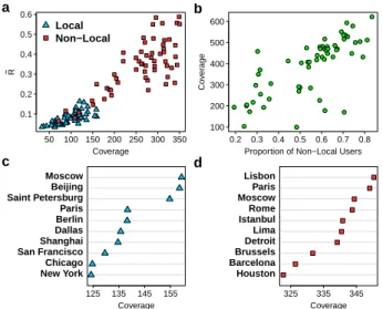
50 100 150 200 250 300 350 0.1 0.2 0.3 0.4 0.5 0.6 Coverage R ~ Local Non−Local a 100 200 300 400 500 600 0.2 0.3 0.4 0.5 0.6 0.7 0.8 Proportion of Non−Local Users
Co v er age b 125 135 145 155 New York Chicago San Francisco Shanghai Dallas Berlin Paris Saint Petersburg Beijing Moscow Coverage c 325 335 345 Houston Barcelona Brussels Detroit Lima Istanbul Rome Moscow Paris Lisbon Coverage d
Figure 5: Relation between local and non-local users. (a) Scatter-plot of ˜R as a function of the cover-age for locals (blue triangles) and non-locals (red squares). (b) Coverage as a function of the proportion of non-local Twitter users. (c) Top 10 ranking cities based only on lo-cal users according to the coverage. (d) The same ranking but based only on the movements of non-local users. In all the cases, the number of local and non-local users ex-tracted is u = 100 for every city and all the metrics are averaged over 100 independent extractions.
We consider a user to be a resident of a city if most of his/her tweets are posted from it. Otherwise, he/she is seen as an external visitor. Residents of the 58 cities we consider have a significantly lower coverage (about 96) than visitors (about 260). This means that the lo-cals move toward more concentrated locations, such as places of work or the residences of family and friends, while visitors have a comparatively higher diversity of origins and destinations.
The difference between locals and non-locals is even more dramatic when the normalized radius, ˜R, for each city is plotted as a function of the coverage for both types of users in Figure5a. Two clusters clearly emerge, showing that the locals tend to move less than
the visitors. Such difference between users is likely to be behind the change of behavior in the temporal evo-lution of the average radius detected in Figure3, and introduces the ratio of visitors over local users as a rel-evant parameter to describe the mobility from a city. Indeed, visitors contribute the most for the radius and the area covered (see Figure5b for the coverage) while residents contribute most to the local relevance of a city (Figure5c for the coverage and Figure S10a in Ap-pendix for ˜R). The top rankers in this classification are Hong Kong and San Francisco in ˜R and Moscow and Beijing in the coverage. All of them are cities that may act as gates for quite extense hinterlands. The rankings based on non-locals (Figures5d for the coverage and Figure S10b in Appendix for ˜R) get us back the more common top rankers such as Paris, New York and Lisbon.
City attractiveness
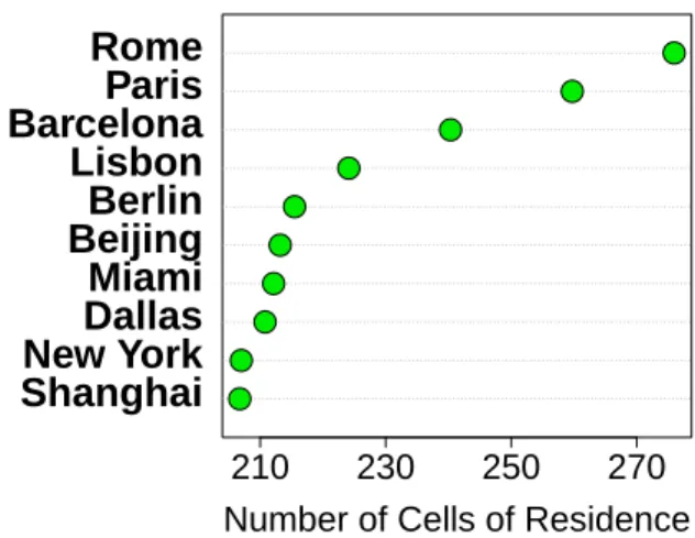
Thus far, we have considered a city as origin and an-alyzed how people visiting it diffuse across the planet. We now consider the attractiveness of a city by taking the opposite point of view and analyzing the origins of each user seen within the confines of a city. We modify the two metrics defined above to consider the normalized average distance of the users’ residences (represented by the centroid of the cell of residence) to the center of the considered city c and the number of different cells where these users come from. In this case, the to metrics are averaged over 100 indepen-dent extractions of u = 1000 Twitter users. The re-sulting rankings depict the attractiveness of each city from the perspective of external visitors: How far are people willing to travel to visit this city? The Top 10 cities are shown in Figure 6 for the coverage (see Figure S11 in Appendix for the normalized average radius). Rome, Paris and Lisbon are also quite con-sistently the top rankers in terms of attractiveness to external visitors.
A network of cities
Finally, we complete our analysis by considering travel between the 58 selected cities. We build a network connecting the 58 cities under consideration where the directed edge from city i to city j has a weight given by the fraction of local Twitter users in the city i which were observed at least once in city j. For simplicity, in what follows, we consider only local users who left their city at least once. This network captures the strength of connections between cities al-lowing us to analyze the communities that naturally arise due to human mobility. Using the OSLOM clus-tering detection algorithm [52, 53] we find 6 commu-nities as shown in Figure7. These communities follow approximately the natural boundaries between conti-nents: two communities in North and Center America,
210
230
250
270
Shanghai
New York
Dallas
Miami
Beijing
Berlin
Lisbon
Barcelona
Paris
Rome
Number of Cells of Residence
Figure 6: City attractiveness. Top 10 cities ranked by the number of distinct cells of residence for u = 1000 Twitter users drawn at random. The metric is averaged over 100 independent extractions.one community in South America, another in Europe, two communities in Asia (Japan and rest of Asia plus Sydney), indicating that they correspond to economic, cultural and geographical proximities. Similar results were obtained using the Infomap [54] cluster detection algorithm, confirming the robustness of the communi-ties detected.
North America
Global Ranking Regional Ranking
1. New York (1) 1. New York
2. Miami (6) 2. Los Angeles
3. San Francisco (8) 3. Chicago 4. Los Angeles (9) 4. Toronto 5. Chicago (18) 5. Detroit
6. Toronto (19) 6. Miami
7. San Diego (23) 7. Dallas 8. Detroit (25) 8. San Francisco 9. Montreal (26) 9. Washington 10. Atlanta (27) 10. Atlanta
Europe
Global Ranking Regional Ranking
1. London (2) 1. London 2. Paris (3) 2. Paris 3. Madrid (10) 3. Moscow 4. Barcelona (11) 4. Barcelona 5. Moscow (16) 5. Berlin 6. Berlin (20) 6. Rome 7. Rome (21) 7. Madrid 8. Amsterdam (24) 8. Lisbon 9. Lisbon (38) 9. Amsterdam
10. Milan (40) 10. Saint Petersburg
TABLE I: Comparison of the regional and the global betweenness rankings. In parenthesis the total global ranking position of each city.
With these empirical communities in hand we can now place each city into a local as well as a global
0 2 4 6 8 10
Los Angeles San FranciscoMiami
SingaporeTokyo Paris London New York Weighted Betwennness (x 102) Weighted degree
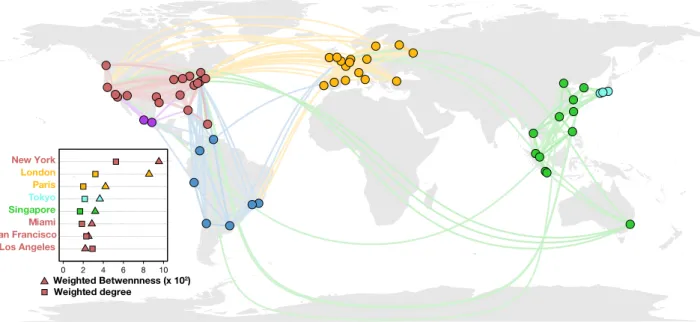
Figure 7: Mobility network. Local Twitter users mobility network between the 58 cities. Only the flows representing the top 95% of the total flow have been plotted. The flows are drawn from the least to the greatest. The inset shows the top 8 cities ranked by weighted betweenness and weighted degree.
context. In a network context, the importance of each node can be measured in different ways. Two classi-cal measures are the strength of a node [55] and the weighted betweenness [56, 57]. Given the way we de-fined our network above, these correspond, roughly, to the fraction of local users that travel out of a city and how important that city is in connecting trav-elers coming from other cities to their final destina-tions. In the inset of the Figure 7, we analyze the ranking resulting from these two metrics and iden-tify New York and London as the most central nodes in terms of degree and betweenness and, particularly, New York for the weighted degree at a global scale. However, when we restrict our analysis to just the regional scene of each community, the relative impor-tance of each city quickly changes. The rankings for the regional weighted degree are similar to the global ones since this metric depends only on the population of each city and not on who it is connected to. The most central cities occupy the same positions except for San Diego, which slipped down three places down. On the other hand, the weighted betweenness is prop-erty that depends strongly on the network topology, a property that can be seen by the dramatic shifts we observe when considering only the local commu-nity of each city with most cities moving several po-sitions up or down (see details in Table II and Ta-ble S2 in Appendix). For example, San Diego went down nine places meaning that this city has a global influence due to the fact that San Diego is a com-munication hub between United States and Central America. Dallas went up six places, indicating that its influence is higher at the regional scale rather than in the international arena. In the same way, Madrid went down four places whereas Barcelona stayed at
the same place, this means that Madrid is more in-fluential than Barcelona at a global scale as an inter-national bridge connecting Europe and Central and South America but not at a regional (European) scale.
DISCUSSION
The study of competition and interactions between cities has a long history in fields such as Geography, Spatial Economics and Urbanism. This research has traditionally taken as basis information on finance ex-changes, sharing of firm headquarters, number of pas-sengers transported by air or tons of cargo dispatched from one city to another. One can define a network relying on these data and identify the so-called World Cities, those with a higher level of centrality as the global economic or logistic centers. Here, we have taken a radically different approach to measure quan-titatively the influence of a city in the world. Nowa-days, geolocated devices generate a large quantity of real time and geolocated data permitting the char-acterization of people mobility. We have used Twit-ter data to track users and classify cities according to the mobility patterns of their visitors. Top cities as mobility sources or attraction points are identified as central places at a global scale for cultural and in-formation interchanges. This definition of city influ-ence makes possible its direct measurement instead of using indirect information such as firm headquar-ters or direct flights. Still, the quality of the results depends on the capacity of geolocated tweets to de-scribe local and global mobility. Indeed, observing the World through Twitter data can lead to possible dis-tortions, economic and sociodemographic biases, the
Twitter penetration rate may also vary from country to country leading to an under-representation of the population, for example, from Africa and from China. The cities selected for this work are those that, on one hand, concentrate large populations and, on the other, enough number of tweets to be part of the analysis. There are biases acting against our work, as the lack of coverage in some areas of the world, and others in favor, such as the fact that younger and wealth-ier individuals are more likely to both travel and use Twitter. The estimated mobility patterns are nat-urally partial since only refer to the selected cities. Still, as long as the users provide a significant sam-ple of the external urban mobility, the flow network is enough for the performed analysis. Furthermore, sev-eral recent works have proven the capacity of geolo-cated tweets to describe human mobility comparing different data sources as information collected from cell phone records, Twitter, traffic measure techniques and surveys [23,24,41].
More specifically and assuming data reliability, we consider the users’ displacements after visiting each city. The urban areas are ranked according to the area covered and the radius traveled by these users as a function of time. These metrics are inspired by the framework developed for random walks and Levy flights, which allows us to characterize the evolution of the system with well-defined mathematical tools and with a clear reference baseline in mind. Previ-ous literature rankings usually find a hierarchy cap-tained by New York and London as the most central world cities. The ranks dramatically change when one has into account users’ mobility. A triplet formed by Rome, Paris and Lisbon consistently appear on the top of the ranking by extension of visitor’s mobility but also by their attractiveness to travelers of very diverse origin. A combination of economic activity appealing to tourism and diversity of links to other lands, in some cases product of recent history, can ex-plain the presence of these cities on the top. These three cities are followed by others such as San Fran-cisco that without being one of the most populated cities in the US extends it influence over the large Pa-cific basin or Hong Kong, Beijing and Shanghai that replicates it on the other side of the Pacific region. These cities are in some cases gates to broad hinter-lands. This is relevant since our metrics have into account the diversity in the visitors’ origins.
These results rely on the full users population, dis-criminating only by the place of residence between lo-cals and non lolo-cals to each city. The influence of cities measured in this way includes their impact in rural as well as in other urban areas. However, the analysis can be restricted to users residing in an urban area
and to their displacements toward other cities. In this way, we obtain a weighted directed network between cities, whose links weights represent the (normalized) fluxes of users traveling from one city to another. This network provides the basis for a more traditional cen-trality analysis, in which we recover London and New York as the most central cities at a global scale. The match between our results and those from previous analysis brings further confidence on the quality of the flow measured from online data. The network framework permits to run clustering techniques and divide the world city network in communities or ar-eas of influence. When the centrality is studied only within each community, we obtain a regional perspec-tive that induces a new ranking of cities. The com-parison between the global and the regional ranking provides important insights in the change of roles of cities in the hierarchies when passing from global to regional.
Summarizing, we have introduced a new method to measure the influence of cities based on the Twitter user displacements as proxies for the mobility flows. The method, despite some possible biases due to the population using online social media, allows for a di-rect measurement of a city influence in the world. We proposed three types of rankings capturing differ-ent perspectives: rankings based on “city-to-world” and “world-to-city” interactions and rankings based on “city-to-city” interaction. It is interesting to note that the most influential cities are very different ac-cording to the perspective and the scale (regional and global). This introduces the possibility of studying re-lations among cities and between cities and rural areas with unprecedented detail and scale.
ACKNOWLEDGEMENTS
Partial financial support has been received from the Spanish Ministry of Economy (MINECO) and FEDER (EU) under projects MODASS (FIS2011-24785) and INTENSE@COSYP (FIS2012-30634), and from the EU Commission through projects EUNOIA, LASAGNE and INSIGHT. The work of ML has been funded under the PD/004/2013 project, from the Con-selleria de Educacin, Cultura y Universidades of the Government of the Balearic Islands and from the Eu-ropean Social Fund through the Balearic Islands ESF operational program for 2013-2017. JJR from the Ram´on y Cajal program of MINECO. BG was par-tially supported by the French ANR project HarMS-flu (ANR-12-MONU-0018).
[1] Christaller W. 1966 Die Zentralen Orte in
S¨uddeutschland: eine Okonomisch-Geographische¨ Untersuchung Uber¨ die Gesetz Massigkeit der
Verbreitung und Entwicklung der Siedlungen mit St¨adtischen Funktionen, Fischer Verlag, Jena (1933). (English translation: Christaller W, Baskin CW.
Central places in Southern Germany, Prentice Hall, Englewood Cliffs NJ.)
[2] Friedmann J, Wolff G. 1982 World city formation: an agenda for research and action. International Jour-nal of Urban and RegioJour-nal Research 6, 309–344. (doi:10.1111/j.1468-2427.1982.tb00384.x)
[3] Berry B. 1964 Cities as systems within a systems of cities. Papers of Regional Science Association 13, 147–163. (doi:10.1111/j.1435-5597.1964.tb01283.x) [4] Knox PL, Taylor PJ. 1995 World cities in a
world-system. Cambridge University Press.
[5] Rimmer P. 1998 Transport and Telecommunications among world cities. In Lo FC, Yeung YM (eds.). Glob-alization and the world of large cities, Tokyo: United Nations University Press, 433–470.
[6] Pumain D. 2000 Settlement systems in the evolution. Geografiska Annaler 82B, 73–97. (doi:10.1111/j.0435-3684.2000.00075.x)
[7] Taylor JP. 2001 Specification of the World City
Network. Geographical Analysis 33, 181–194.
(doi:10.1111/j.1538-4632.2001.tb00443.x)
[8] Derudder B, Taylor PJ, Witlox F, Catalano G. 2003 Hierarchical tendencies and regional patterns in the world city network: A global urban anal-ysis of 234 cities. Regional Studies 37, 875–886. (doi:10.1080/0034340032000143887)
[9] Derudder B, Witlox F. 2004 Assessing central places in a global age: on the networked localization strate-gies of advances producer services. J. Retailing and Consumer Services 11 171–180. (doi:10.1016/S0969-6989(03)00023-7)
[10] Brown E, Derudder B, Parnreiter C, Pelupessy W, Taylor PJ, Witlox F. 2010 World City Networks and Global Commodity Chains: towards a world-systems’ integration. Global Networks 10, 1470–2266. (doi:10.1111/j.1471-0374.2010.00272.x)
[11] Bassens D, Derudder B, Witlox F. 2010 Search-ing for the Mecca of finance: Islamic financial ser-vices and the world city network. Area 42, 35–46. (doi:10.1111/j.1475-4762.2009.00894.x)
[12] Neal Z. 2011 Differentiating centrality and power in the world city network. Urban Studies 48, 2733–2748. (doi:10.1177/0042098010388954)
[13] Zook MA, Brunn SD. 2005 Hierarchies, Regions and Legacies: European cities and global commercial pas-senger air travel. J. Contemporary European Studies 13, 203–220. (doi:10.1080/14782800500212459) [14] Derudder B, Witlox F. 2005 On the use of
inad-equate airline data in mappings of a global urban system. J. Air Transport Management 11, 231–237. (doi:10.1016/j.jairtraman.2005.01.001)
[15] Derudder B, Witlox F. 2008 Mapping world city networks through airline flows: context, relevance, an problems. J. Transport Geography 16, 305–312. (doi:10.1016/j.jtrangeo.2007.12.005)
[16] Allen J. 2010 Powerful city networks: More
than connections, less than domination and
control. Urban Studies 47, 2895–2911. (doi:
10.1177/0042098010377364)
[17] Brockmann D, Hufnagel L, Geisel T. 2006 The scal-ing laws of human travel. Nature 439, 462–465. (doi:10.1038/nature04292)
[18] Gonzalez MC, Hidalgo CA, Barabasi A-L. 2008 Un-derstanding individual human mobility patterns. Na-ture 453, 779–782. (doi:10.1038/naNa-ture06958) [19] Balcan D, Colizza V, Gon¸calves B, Hu H,
Ram-asco JJ, Vespignani V. 2009 Multiscale mobility net-works and the spatial spreading of infectious dis-eases. Proc. Natl. Acad. Sci. USA 106, 21484–21489. (doi:10.1073/pnas.0906910106)
[20] Noulas A, Scellato S, Lambiotte R, Pontil M, Mas-colo C. 2012 A tale of many cities: Universal pat-terns in human urban mobility. PloS one 7, e37027. (doi:10.1371/journal.pone.0037027)
[21] Bagrow JP, Lin Y-R. 2012 Mesoscopic structure and social aspects of human mobility. PLoS ONE 7, e37676. (doi:10.1371/journal.pone.0037676)
[22] Grabowicz PA, Ramasco JJ, Goncalves B, Eguiluz
VM. 2014 Entangling mobility and
interac-tions in social media. PLoS ONE 9, e92196.
(doi:10.1371/journal.pone.0092196)
[23] Lenormand M, Picornell M, Garcia Cant´u O, Tu-gores A, Louail T, Herranz R, Barthelemy M, Fr´ıas-Mart´ınez E, Ramasco JJ. 2014 Cross-checking dif-ferent source of mobility information. PLoS ONE 9, e105184. (doi:10.1371/journal.pone.0105184)
[24] Tizzoni M, Bajardi P, Decuyper A, Kon Kam King G, Schneider CM, Blondel V, Smoreda Z, Gonzlez MC, Colizza V. 2014 On the use of human mobility proxy for the modeling of epi-demics. PLoS Computational Biology 10, e1003716. (doi:10.1371/journal.pcbi.1003716)
[25] Jurdak R, Zhao K, Liu J, AbouJaoude M,
Cameron M, Newth D. 2014 Understanding hu-man mobility from Twitter. Available online at http://arxiv.org/abs/1412.2154.
[26] Java A, Song X, Finin T, Tseng B. 2007 Why we twitter: understanding microblogging usage and communities. In Proceedings of the 9th ACM WebKDD and 1st SNA-KDD 2007 workshop on Web mining and social network analysis, 56–65. (doi:10.1145/1348549.1348556)
[27] Krishnamurthy B, Gill P, Arlitt M. 2008 A few chirps about twitter. In WOSP ’08: ACM Proceedings of the first workshop on Online social networks, 19–24. (doi:10.1145/1397735.1397741)
[28] Huberman BA, Romero DM, Wu F. 2008
Social networks that matter: Twitter
un-der the microscope. First Monday 14.
(http://firstmonday.org/article/view/2317/2063)
[29] Grabowicz PA, Ramasco JJ, Moro E, Pujol
JM, Eguiluz VM. 2012 Social features of on-line networks: The strength of intermediary ties
in online social media. PLoS ONE 7, e29358.
(doi:10.1371/journal.pone.0029358)
[30] Ferrara E, Varol O, Menczer F, Flammini A. 2013 Traveling trends: social butterflies or frequent fliers? In Proceedings of the first ACM Conference on On-line Social Networks COSN ’13, 213–222, New York. (doi:10.1145/2512938.2512956)
[31] Reades J, Calabrese F, Sevtsuk A, Ratti C.
2007 Cellular census: Explorations in urban
data collection. Pervasive Computing 6, 30–38. (doi:10.1109/MPRV.2007.53)
[32] Reades J, Calabrese F, Ratti C. 2009
Eigen-places: analysing cities using the space-time struc-ture of the mobile phone network. Environment and Planning B: Planning and Design 36, 824–836. (doi:10.1068/b34133t)
[33] Cheng Z, Caverlee J, Lee, K. 2010 You Are
Where You Tweet: A Content-based Approach
19th ACM International Conference on
Informa-tion and Knowledge Management 17, 759-768.
(doi:10.1080/10095020.2014.941316)
[34] Soto V, Fr´ıas-Mart´ınez E. 2011 Automated land use identification using cell-phone records, Procs. of the ACM conference HotPlanet’11 17–22, New York. (doi:10.1145/2000172.2000179)
[35] Fr´ıas-Mart´ınez V, Soto V, Hohwald H, Fr´ıas-Mart´ınez E. 2012 Characterizing urban landscapes using ge-olocated tweets. In SOCIALCOM-PASSAT ’12 Pro-ceedings of the 2012 ASE/IEEE International Con-ference on Social Computing and 2012 ASE/IEEE International Conference on Privacy, Security, Risk and Trust, 239–248. (doi:10.1109/SocialCom-PASSAT.2012.19)
[36] Noulas A, Mascol C, Frias-Martinez E. 2013 Exploit-ing Foursquare and Cellular Data to Infer User Ac-tivity in Urban Environments, Procs. MDM ’13, 167– 176.
[37] Louail T, Lenormand M, Garcia Cant´u O, Picor-nell M, Herranz R, Fr´ıas-Mart´ınez E, Ramasco JJ, Barthelemy M. 2014 From mobile phone data to the spatial structure of cities. Scientific Reports 4, 5276. (doi:10.1038/srep05276)
[38] Grauwin S, Sobolevsky S, Moritz S, Godor I, Ratti C. 2015 Towards a comparative science of cities: us-ing mobile traffic records in New York, London and Hong Kong. In Helbich M, Jokar Arsanjani J, Leitner M (Eds.) Computational Approaches for Urban Envi-ronments 13, 363–387.
[39] Fran¸ca U, Sayama H, McSwiggen C,
Danesh-var R, Bar-Yam Y. 2014 Visualizing the ”Heart-beat” of a City with Tweets. Available online at http://arxiv.org/abs/1411.0722.
[40] Louail T, Lenormand M, Picornell M, Garcia Cant´u O, Herranz R, Fr´ıas-Mart´ınez E, Ramasco JJ, Barthelemy M. 2015 Uncovering the spatial struc-ture of mobility networks. Nastruc-ture Communications 6, 6007. (doi:10.1038/ncomms7007)
[41] Lenormand M, Tugores A, Colet P, Ramasco JJ. 2014 Tweets on the road. PLoS ONE 9, e105407. (doi:10.1371/journal.pone.0105407)
[42] Bettencourt L, Lobo J, Helbing D, Kuhnert C, West G. 2007 Growth, innovation, scaling, and the pace of life in cities. Proc. Natl. Acad. Sci. USA 104, 7301– 7306. ( doi: 10.1073/pnas.0610172104)
[43] Batty M. 2008 The Size, Scale, and Shape of Cities. Science 319, 769–771. (doi:10.1126/science.1151419)
[44] Bettencourt L, West G. 2010 A unified
the-ory of urban living. Nature 467, 912–913.
(doi:10.1038/467912a)
[45] Bettencourt L. 2013 The Origins of
Scal-ing in Cities. Science 340, 1438–1441.
(doi:10.1126/science.1235823)
[46] Adnan A, Leak A, Longley P. 2014 A geocomputa-tional analysis of Twitter activity around different world cities. Geo-spatial Information Science 17, 145-152. (doi:10.1080/10095020.2014.941316)
[47] Batty M. 2013 The New Science of Cities. The MIT Press.
[48] Hawelka B, Sitko I, Beinat E, Sobolevsky S, Kaza-kopoulos P, Ratti C. 2014 Geo-located twitter as a proxy for global mobility patterns. Cartography and Geographic Information Science 41, 260–271. (doi:10.1080/15230406.2014.890072)
[49] Oliveira EA, Andrade Jr JS, Makse HA. 2014 Large
cities are less green. Scientific Reports 4, 4235. (doi:10.1038/srep04235)
[50] Arcaute E, Hatna E, Ferguson P, Youn H, Jo-hansson A, Batty M. 2015 Constructing cities, de-constructing scaling laws. J. R. Soc. Interface 12. (doi:10.1098/rsif.2014.0745)
[51] Weiss, GH. 1994 Aspects and Applications of the Ran-dom Walk. North-Holland Publishing Co.
[52] Lancichinetti A, Radicchi F, Ramasco JJ.
2010 Statistical significance of
communi-ties in networks. Phys. Rev. E 81, 046110.
(doi:10.1103/PhysRevE.81.046110)
[53] Lancichinetti A, Radicchi F, Ramasco JJ, For-tunato S. 2011 Finding Statistically Significant Communities in Networks. PLoS ONE 6, e18961. (doi:10.1371/journal.pone.0018961)
[54] Rosvall M, Bergstrom CT. 2008 Maps of random walks on complex networks reveal community struc-ture. Proc. Natl. Acad. Sci. USA 105, 1118–1123. (doi:10.1073/pnas.0706851105)
[55] Barrat A, Barthelemy M, Pastor-Satorras R, Vespig-nani A. 2004 The architecture of complex weighted networks. Proc. Natl. Acad. Sci. USA 101, 3747–3752. (doi:10.1073/pnas.0400087101)
[56] Newman MEJ. 2001 Scientific collaboration
networks. II. Shortest paths, weighted
net-works, and centrality. Phys. Rev. E 64, 016132. (doi:10.1103/PhysRevE.64.016132)
[57] Brandes U. 2001 A faster algorithm for
be-tweenness centrality. J. Math. Soc. 25, 163–177. (doi:10.1.1.11.2024)
APPENDIX
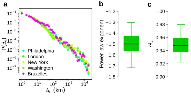
As a first characterization of the data, we have computed the great circle distance ∆r between successive
positions of the same Twitter user living in one of the 58 cities (Figure S1). The distribution P (∆r) for each
city is well approximated by a power law with an average exponent value of 1.5. These results are consistent with the exponent obtained in other studies [17,18,48]. It is interesting to note that the distributions are very similar for all the cities.
● ● ● ●●●● ●●●● ●●● ●● ● ● ●●●●● ● ● ●●● ●●● ●●●● ●● ● ● ● ●●● ● ●● ● ● ● ●● ●●●●● ●●● ●● ●●● ● ●● ●●●● ●●● ●● ● ●●●● ● ●● ●● ● ● ●●● ● ● ● ● ● ●●●●●● ●●●● ● ● ●● ● ● ●● ●●● ●●●● ●● ●●●●●● ●● ● ● ● ● ●● ●●● ● ● ● ●● ●●●●●●●● ●● ● ● ● ● ●● ●●●●●●● ●●● ●● ●●●● ● ● ● ●●●● ●● ● ● ● ● ●● ●●● ●●●●●●● ●●●● ●● ●● ●● ●●● ●●●● ●● ● ●● ● ● ●● ● ●●● ● ● ●
∆
r(
km
)
P
(
∆
r)
10
010
110
210
310
410
−710
−610
−510
−410
−310
−210
−1 ● ● ● ● ●Philadelphia
London
New York
Washington
Bruxelles
a
−1.8
−1.7
−1.6
−1.5
−1.4
−1.3
−1.2
P
o
w
er la
w e
xponent
b
0.90
0.92
0.94
0.96
0.98
1.00
R
2c
Figure S1: Probablity density function of distance travelled by the local Twitter users. (a) Probablity density function P (∆r) of the distance travelled by the local Twitter users for 5 cities drawn at random among the 58
case studies. ∆r is the great circle distance between each successive position of the local Twitter users. (b) Boxplot of
the 58 power-law exponent. (c) Boxplot of the R2. The boxplot is composed of the minimum value, the lower hinge, the
median, the upper hinge and the maximum value.
200
400
600
800
1000
0
200
400
600
800
∆
t(day)
Number of activ
e users
●
(350,300)
Figure S2: Minimum number of active users as a function of ∆t (blue line). The gray lines represent the
● ●● ● ●●● ● ● ●● ● ● ● ● ● ●● ● ● ● ● ● ● ● ● ● ● ● ● ● ●●● ● ● ● ●●● ● ● ● ●● ● ●● ● ● ●● ● ● ● ● ● ● ● ● ● ● ● ● ● ● ●● ● ● ● ●●● ● ● ●●● ●● ● ● ● ●● ● ● ● ● ● ● ● ●● ● ● ●● ● ● ● ● ●
R (km)
P
(
R
)
10
010
110
210
310
410
−610
−510
−410
−310
−2a
● ● ● ● ●Rome
Paris
New York
Lisbon
London
●●● ● ●● ● ● ●● ● ●● ● ● ● ● ● ●● ● ● ● ● ● ● ● ● ● ● ● ●● ● ● ● ● ● ● ● ● ● ● ● ● ● ●● ● ● ● ● ●● ●● ●●Ranking Average
Ranking Median
0
10
20
30
40
50
60
0
10
20
30
40
50
60
b
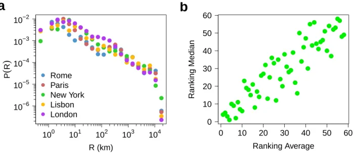
Figure S3: Radius. (a) Probablity density function of the radius per Twitter users for 5 cities. (b) Ranking by median radius as a function of the ranking by average radius. The rankings are based on an average of the two statistics over 100 independent extractions of a set of u = 300 users.
70
80
90
100
110
120
Toronto
MontrealDetroit
Chicago
New YorkBoston
PhiladelphiaWashington AtlantaDallas Dublin ManchesterHouston London AmsterdamBrussels VancouverParis Miami Phoenix StockholmBerlin Los Angeles
San FranciscoSan Diego
Madrid
LisbonMilan
Barcelona
Saint PetersburgRome
Mexico Guadalajara
Santo DomingoMoscow
Istanbul CaracasBogota Lima BeijingSeoul Tokyo NagoyaOsaka
Rio de JaneiroSao Paulo
ShanghaiTaipei
Hong KongSantiago
Buenos AiresBangkok
Manila
Kuala LumpurSingapore
Jakarta
BandungSydney
Average Distance (x 10
3
km)
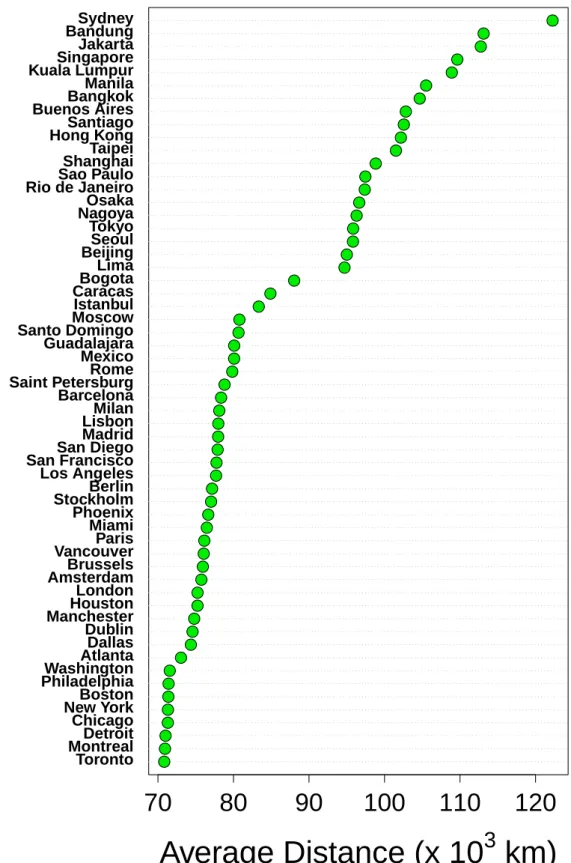
Figure S4: Ranking of the cities according the the average distance between the center of the city and all the Twitter users’ place of residence (represented by the centroid of the cell of residence).
∆
t(days)
R (km)
100 101 102 103 101 102 103 104a
∆
t(days)
R (km)
100 101 102 103 101 102 103 104b
Hong Kong Paris London Detroit BandungFigure S5: Evolution of the average radius for the local users (a) and for the non-local users (b). Each curve represents the evolution of the average radius R averaged over 100 independent extractions of a set of u = 100 users as a function of the number of days ∆tsince the first passage in the city. In order to show the general trend, each
gray curve corresponds to a city. The evolution of the radius for several cities is highlighted, such as the top and bottom rankers or representatives of the two main detected behaviors.
0.1
0.2
0.3
0.4
0.5
100
200
300
400
500
600
R
~
Coverage
Figure S6: Coverage as a function of ˜R for the 58 cities. A certain level of correlation can be observed between both metrics. Both metrics are averaged over 100 independent extractions of a set of u = 300 users.
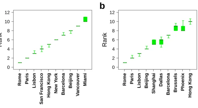
0 5 10 15
Rank
Rome Paris Lisbon
San Francisco Hong K ong Ne w Y ork Bar celona Beijing V ancouver Miami
a
0 5 10 15 20 25Rank
Rome Paris Lisbon
Beijing Shanghai Dallas Bar celona Brussels Phoenix Hong K ong
b
Figure S7: Variations of the rankings over 100 realizations. (a) Ranking for the normalized average radius. (b) Ranking for the coverage. The boxplot is composed of the minimum value, the lower hinge, the median, the upper hinge and the maximum value. The rankings are averaged over 100 independent extractions of a set of u = 300 users.
0 2 4 6 8 10 12
Rank
Rome P aris Lisbon San Francisco Hong K ong Ne w Y ork Bar celona Beijing V ancouver Miamia
0 2 4 6 8 10 12Rank
Rome P aris Lisbon Beijing Shanghai Dallas Bar celona Brussels Phoenix Hong K ongb
Figure S8: Variations of the rankings over 10 realizations performed on the average over 10 realizations. (a) Ranking for the normalized average radius. (b) Ranking for the coverage. The boxplot is composed of the minimum value, the lower hinge, the median, the upper hinge and the maximum value. The rankings are averaged over 100 independent extractions of a set of u = 300 users.
Entropy index
The natural way of taking the heterogeneity of visiting frequencies into consideration is to introduce an entropy measure. If we define the probability pti than an individual tweet originating from the users we are considering originated in a cell i, then the entropy S for a given time interval ∆t is given by:
S (t) = − PN i=1p t ilog(pti) log (N (t)) (1)
where the normalizing factor N (t), the number of cells with non-zero number of tweets, corresponds to the uniform case where each tweet has the same probability of being produced within each cell. With this normalization, the entropy is defined to vary just between 0 and 1, regardless of the number of cells and tweets we might consider in each case.
The entropy as a function of the number of visited cells is plotted in Figure7a. The entropy enhances with the number of visited cells despite the normalization, which implies that the tweets tend to distribute more uniformly for those cities with larger areas covered and therefore with a larger global projection. Besides the general trend, there are some interesting outliers such as Moscow and Saint Petersburg, with a high area covered given the size of Russia but low entropy meaning that the travels concentrate toward a few cells (likely the cities in a vast territory). On the other extreme, we find Osaka and Nagoya with a low are covered but high entropy. A possible reason is that the travels can be mostly within Japan but since the population in the country is well distributed, the trip destinations are well mixed.
As can be seen in Figure7b, the entropy measured in the cities based only in local users is way lower than for the non-locals. This means that the locals move toward more concentrated locations, in contrast to the comparatively higher diversity of origins of the non-local visitors.
0.4
0.5
0.6
0.7
100 200 300 400 500 600
Coverage
E
nt
ro
py
a
Moscow
Osaka
Nagoya
Saint Petersburg
0.1
0.2
0.3
0.4
0.5
0.6
0.7
E
nt
ro
py
Local
Non Local
b
Figure S9: Entropy index according to the Twitter user type. (a) Entropy index as a function of the number of cells visited by u = 300 Twitter users drawn at random. (b) Box plot with the entropy measured for the different cities separating the users as locals and non-locals. The number of users is u = 100 in this case.
0.12
0.14
0.16
Taipei
Rome
London
Beijing
New York
Vancouver
Sydney
Paris
San Francisco
Hong Kong
R
~
a
0.48
0.52
0.56
0.60
Beijing
Barcelona
Hong Kong
Sydney
San Francisco
Lisbon
Vancouver
Rome
New York
Paris
R
~
b
Figure S10: Relation between local and non-local users. (a) Top 10 ranking cities based only on local users according to the average radius. (b) Top 10 ranking cities based only on non-local users according to the average radius. In all the cases, the number of local and non-local users extracted is u = 100 for every city and all the metrics are averaged over 100 independent extractions.
0.30
0.35
0.40
0.45
Shanghai
New York
Dallas
Miami
Beijing
Berlin
Lisbon
Barcelona
Paris
Rome
Average Distance (km)
Figure S11: City attractiveness. Top 10 cities ranked by the average distance between the Twitter users’ residences (represented by the centroid of the cell of residence) and the city center for u = 1000 Twitter users drawn at random. The metric is averaged over 100 independent extractions.
Table SI: Description of the case studies
City Number ofusers Number ofTweets
Number of Tweets per user Amsterdam 2661 305363 114.75 Atlanta 2863 296390 103.52 Bandung 5620 405241 72.11 Bangkok 2604 239514 91.98 Barcelona 1713 165934 96.87 Beijing 1299 131922 101.56 Berlin 678 45238 66.72 Bogota 2226 213739 96.02 Boston 752 73561 97.82 Brussels 1243 97688 78.59 Buenos Aires 411 28500 69.34 Caracas 3625 375933 103.71 Chicago 2191 257572 117.56 Dallas 1214 128834 106.12 Detroit 13608 938524 68.97 Dublin 704 78434 111.41 Guadalajara 721 57031 79.10 Hong Kong 1098 108203 98.55 Houston 1582 186830 118.10 Istanbul 1321 103117 78.06 Jakarta 1919 196188 102.23 Kuala Lumpur 509 42665 83.82 Lima 360 42186 117.18 Lisbon 6782 698998 103.07 London 6392 580084 90.75 Los Angeles 1760 159781 90.78 Madrid 1566 202650 129.41 Manchester 1792 163090 91.01 Manila 4118 293015 71.15 Mexico 2534 247486 97.67 Miami 688 84544 122.88 Milan 666 61175 91.85 Montreal 1239 133461 107.72 Moscow 2334 263132 112.74 Nagoya 9668 892442 92.31 New York 4044 398769 98.61 Osaka 2567 247449 96.40 Paris 432 43301 100.23 Philadelphia 2206 247159 112.04 Phoenix 1380 150468 109.03 Rio de Janeiro 3292 352777 107.16 Rome 824 88402 107.28 Saint Petersburg 497 51601 103.82 San Diego 1810 182035 100.57 San Francisco 4628 419032 90.54 Santiago 2471 250639 101.43 Santo Domingo 302 20245 67.04 Sao Paulo 6479 653909 100.93 Seoul 1898 152666 80.44 Shanghai 526 49282 93.69 Singapore 3501 288267 82.34 Stockholm 745 106366 142.77 Sydney 1176 121426 103.25 Taipei 485 40259 83.01 Tokyo 10333 844602 81.74 Toronto 1476 135914 92.08 Vancouver 796 70018 87.96 Washington 3755 421374 112.22
Table SII: Comparison of the regional and the global betweenness rankings.
Community Global Ranking Regional Ranking
North America 1. New York (1) 1. New York
2. Miami (6) 2. Los Angeles
3. San Francisco (8) 3. Chicago
4. Los Angeles (9) 4. Toronto
5. Chicago (18) 5. Detroit
6. Toronto (19) 6. Miami
7. San Diego (23) 7. Dallas
8. Detroit (25) 8. San Francisco
9. Montreal (26) 9. Washington 10. Atlanta (27) 10. Atlanta 11. Washington (29) 11. Phoenix 12. Vancouver (35) 12. Vancouver 13. Dallas (36) 13. Montreal 14. Phoenix (46) 14. Boston 15. Boston (47) 15. Houston
16. Houston (48) 16. San Diego
17. Philadelphia (50) 17. Philadelphia
18. Santo Domingo (58) 18. Santo Domingo
Europe 1. London (2) 1. London
2. Paris (3) 2. Paris 3. Madrid (10) 3. Moscow 4. Barcelona (11) 4. Barcelona 5. Moscow (16) 5. Berlin 6. Berlin (20) 6. Rome 7. Rome (21) 7. Madrid 8. Amsterdam (24) 8. Lisbon 9. Lisbon (38) 9. Amsterdam
10. Milan (40) 10. Saint Petersburg
11. Brussels (41) 11. Dublin
12. Istanbul (42) 12. Istanbul
13. Saint Petersburg (45) 13. Manchester
14. Dublin (49) 14. Brussels
15. Manchester (51) 15. Milan
16. Stockholm (57) 16. Stockholm
Asia 1. Singapore (5) 1. Singapore
2. Hong Kong (7) 2. Hong Kong
3. Taipei (13) 3. Jakarta
4. Jakarta (15) 4. Bangkok
5. Kuala Lumpur (22) 5. Shanghai
6. Seoul (30) 6. Taipei
7. Bangkok (31) 7. Sydney
8. Shanghai (32) 8. Kuala Lumpur
9. Beijing (33) 9. Seoul
10. Sydney (34) 10. Manila
11. Manila (43) 11. Bandung
12. Bandung (56) 12. Beijing
South America 1. Buenos Aires (12) 1. Buenos Aires
2. Sao Paulo (14) 2. Sao Paulo
3. Bogota (28) 3. Bogota
4. Santiago (37) 4. Rio de Janeiro
5. Rio de Janeiro (39) 5. Santiago
6. Lima (44) 6. Caracas
7. Caracas (55) 7. Lima
Japan 1. Tokyo (4) 1. Tokyo
2. Osaka (53) 2. Osaka
3. Nagoya (54) 3. Nagoya
Mexico 1. Mexico (17) 1. Guadalajara