Experimental and numerical study of the mechanical behavior of metal/polymer multilayer composite for ballistic protection

HAL Id: tel-01719634

https://tel.archives-ouvertes.fr/tel-01719634

HAL is a multi-disciplinary open access archive for the deposit and dissemination of sci-entific research documents, whether they are pub-lished or not. The documents may come from teaching and research institutions in France or abroad, or from public or private research centers.

L’archive ouverte pluridisciplinaire HAL, est destinée au dépôt et à la diffusion de documents scientifiques de niveau recherche, publiés ou non, émanant des établissements d’enseignement et de recherche français ou étrangers, des laboratoires publics ou privés.

Experimental and numerical study of the mechanical

behavior of metal/polymer multilayer composite for

ballistic protection

Charles Francart

To cite this version:

Charles Francart. Experimental and numerical study of the mechanical behavior of metal/polymer multilayer composite for ballistic protection. Mechanics of materials [physics.class-ph]. Université de Strasbourg, 2017. English. �NNT : 2017STRAD033�. �tel-01719634�

UNIVERSITÉ DE STRASBOURG

ÉCOLE DOCTORALE ED269

ICUBE – Equipe MMB

THÈSE

Charles FRANCART

soutenue le : 13th _{Octobre 2017}

pour obtenir le grade de :

Docteur de l’université de Strasbourg

: Mécanique des Matériaux

Experimental and numerical study of the

mechanical behavior of metal/polymer

multilayer composite for ballistic protection

THÈSE dirigée par :

Mr AHZI Said Pr., ICUBE – Université de Strasbourg

Mme BAHLOULI Nadia Pr., ICUBE – Université de Strasbourg

RAPPORTEURS :

Mr LAURO Franck Pr., LAMIH – Université de Valenciennes

Mr RUSINEK Alexis Pr., LEM3 – Université de Lorraine

AUTRES MEMBRES DU JURY :

Mme DEMARTY Yaël Dr., French-German Institute of Saint-Louis (ISL)

Mr RITTEL Daniel Pr., Technion (Israël)

2

Symbol Signification Unit

Fitting parameter of kinetic of microstructure change - Empirical coefficient for Taylor equation - Preexponential parameter for damage evolution MPa Burger’s vector (metals)

Temperature sensitivity of locking parameter (polymers)

nm K-1

Plastic modulus MPa

Exponential parameter for damage evolution -

Specific heat J.kg-1_.K-1

Sound velocity m.s-1

Rubber modulus MPa

First parameter of William-Lundon-Ferry relation - Second parameter of William-Lundon-Ferry relation K Damage variable

Diameter of the projectile

- mm

Interdislocation distance nm

, , ,

Triaxiality sensitivity parameters of the plastic strain at initiation of

failure ( for epoxy resin only) -

Grain size µm

Young’s modulus GPa

〈 〉 Average Young’s modulus (in case of viscoelasticity) GPa

Damage energy MPa

True elastic strain -

True plastic strain -

Nominal strain -

Plastic strain at initiation of failure -

Plastic strain at ultimate failure -

Plastic strain at initiation of failure at low strain rate in

shear-compression state of stress -

Minimum limit value of plastic strain at initiation of failure at high

strain rates for polymers materials -

! Elastic strain rate s-1

3 ! Reference strain rate of the calorific model (metals)

Reference strain rate of the cooperative model (polymers) s

-1

! Reference strain rate of the elastic modulus model s-1

!

" Reference strain rate of the stress model s-1

! Athermal transition strain rate s-1

! Reference strain rate for the failure model s-1

# Stress loss during per Kelvin adiabatic heating Pa.K-nT

%& Strain hardening function MPa

%' Strain rate sensitivity function of internal stress -

%(∗ State of stress sensitivity function of plastic strain at initiation of

failure -

%* Strain rate sensitivity function of plastic strain at initiation of failure -

%+, Temperature sensitivity function of plastic strain at initiation of failure -

%# Adiabatic heating sensitivity function -

- Adimensional energy of thermo-activation of overcoming of Peierls

barriers -

. Total energy required to overcome the obstacles through thermal

activation for one atom eV

/ Shear strain -

0 Target thickness mm

ℎ Depth of penetration of the projectile in the target mm

ℎ Limit value of ℎ for plug detachment mm

Δ0 Enthalpy of activation of 3 relaxation phenomenon of polymers kJ.mol-1 4 Third invariant of stress deviator MPa3

5 Average coefficient of annihilation of dislocations -

6 Kocks formula parameter -

57 Boltzmann’s constant 5₇= 1.381= − 23 m2_.kg.s-2_.K-1

6 Kocks formula parameter -

@* Phenomenological parameter of internal stress strain rate sensitivity -

@* Phenomenological parameter of strain rate sensitivity of plastic strain

at initiation of failure -

A Effective projectile length mm

B Stretch parameter -

C Shear modulus GPa

4 E

Temperature sensitivity for Johnson-Cook model (metals) Temperature sensitivity for cooperative model (polymers)

Temperature sensitivity for strain at initiation of failure (polymers)

-

F Elastic Poisson’s ratio -

F Plastic Poisson’s ratio -

Number of change of microstructure for calorific ratio (metals)

Locking parameter (polymers) -

G

Value of parameter for the type of microstructure change in calorific ratio (0 or 1)

Parameter of cooperative model (polymers)

-

G Isotropic hardening coefficient -

G+ Adiabatic heating sensitivity -

G* Phenomenological parameter of internal stress strain rate sensitivity -

G*

Phenomenological parameter of strain rate sensitivity of plastic strain

at initiation of failure -

Ω Calorific ratio (stress modeling) -

℧ = ΩJ _{Inverse calorific ratio (failure modeling) -}

K Kocks’ formula parameter -

K Attempt frequency (Debye frequency) s-1 L Temperature of microstructural change strain rate sensitivity K

M Normalized energetic balance function (polymers) -

N _{- C}57 K-1

O Kinematic hardening coefficient

Perfect gas constant O = 8.314

MPa J.mol-1_.K-1

Q Volumetric mass of the material kg.m-3

QR Equivalent volumetric mass of the target kg.m-3 Q Equivalent volumetric mass of the projectile kg.m-3

Q Density of mobile dislocations m-2

S True plastic stress MPa

ST True equivalent stress MPa

SU Experimental stress MPa

S Nominal stress MPa

S True elastic stress MPa

5

S Effective stress (metals) MPa

SVRW Athermal stress (metals) MPa

SRW Thermal stress (metals) MPa

SX' Viscous drag stress (metals) MPa

S7 Back stress from hyperelasticity phenomenon (polymers) MPa

SY Yield stress (polymers) MPa

S" Effective resistive stress of the target MPa

Z Absolute temperature K

[ Time s

Z Critical temperature (metals) K

Z Melting temperature (metals) K

Z Temperature of microstructural change (metals) – calorific model K

Z" Reference temperature of the considered model K

ZR

Range of temperature of microstructural change – calorific ratio and

cooperative model) K

Z Glass transition temperature (polymers) K or °C

Z\ Temperature of 3 relaxation phenomenon (polymers) K or °C

Z] Temperature of / relaxation phenomenon (polymers) K or °C

Z^ Temperature of degradation (polymers) K or °C

Z Initial temperature K

_ True shear stress MPa

`∗ _{Homologous temperature of the elastic modulus model -}

` Homologous temperature of the calorific model -

a Activation volume for chains crawling (polymers) m3 b Phenomenological parameter of internal stress strain rate sensitivity -

b Phenomenological parameter of strain rate sensitivity of plastic strain

at initiation of failure -

a Impact velocity of the projectile m.s-1

a" Residual velocity of the projectile m.s-1

a Plug velocity m.s-1

ac Theoretical ballistic limit velocity m.s-1

d Taylor-Quinney coefficient -

e Yield stress (metals) MPa

6

e" Reference yield stress at "! and Z_" MPa

f Normalized third stress invariant -

7

INTRODUCTION ... 8

CONSTITUTIVE BEHAVIOR OF METALLIC AND POLYMER MATERIALS ... 12

Description of strain mechanisms ... 15

Constitutive modeling of mechanical behavior ... 39

Description of failure mechanisms ... 60

Constitutive modeling of failure behavior ... 66

MECHANICAL CHARACTERIZATION OF METALLIC AND POLYMER MATERIALS ... 78

Descriptions of the materials ... 81

Descriptions of the experimental tests ... 88

Analysis of the mechanical behavior of the materials ... 97

Analysis of the failure and damage behavior of the materials... 120

CONCLUSION OF THE CHAPTER ... 149

CONSTITUTIVE MODELING OF MECHANICAL BEHAVIOR ... 155

Constitutive modeling of elastic behavior ... 158

Constitutive modeling of inelastic behavior ... 162

Constitutive modeling of the strain at initiation of failure ... 187

Constitutive modeling of the damage evolution ... 196

CONCLUSION OF THE CHAPTER ... 198

NUMERICAL VALIDATION OF MODELING THROUGH APPLICATION TO BALL IMPACT ... 201

A. Experimental performing of ball impacts ... 203

B. Simulation parameterization ... 208

C. Monolayer cases ... 210

D. Application to numerical modeling of multilayer targets ... 237

E. CONCLUSION OF THE CHAPTER ... 252

CONCLUSION ... 256

8

INTRODUCTION

9

Nowadays, one of the main issues addressed to the industry of transportation consists into the development of lightweight materials aiming to reduce fuel consumption and increase the autonomy of the vehicles. This problematic is also pertinent in the military industry for strategic purposes. Indeed, the higher the autonomy of the vehicles is, the larger their area of action will become. Therefore, the development of lightweight protective materials are currently under investigation. This work concerns more precisely light structures submitted to extreme conditions undergone during an impact loading. This study aims to develop a numerical model (using ABAQUS®/Explicit) allowing the evaluation of the dynamic mechanical response of a sintered polymer/metal multilayer composite due to high velocity impact. Both materials have been sintered using Spark Plasma Sintering process (SPS) and are developed at the French-German Institute of Saint-Louis (ISL). This work has for objective to evaluate their protective potential. The metallic material is a sintered 7020 aluminum alloy [1] which can be compared to the commercial AA7020-T651 aluminum alloy, well-known for its efficiency as a ballistic protection. The polymer is a thermoplastic amorphous sintered polyimide [2]. The polyimide presents very high mechanical properties (for a polymer) and thermal stability with a temperature of glass transition around 310 °C. The density of the sintered polyimide is around half of the one of the aluminum alloy; leading to high potential improvement to mass reduction. The sintered aluminum alloy and thermoplastic polyimide layers are assembled together using an epoxy resin. Besides, the multilayer composite has to be designed in order to keep a high level of mechanical performances for diverse kind of solicitations encountered during an impact loading [3]. For this purpose, the stacking sequence of the layers, their number and their respective thicknesses have to be numerically investigated to optimize the efficiency and the cost of the study by keeping the experimental impact tests for the validation of the numerical model. The mechanical behavior of the epoxy resin interface is addressed by considering the presence of this material as an interlayer possessing its own material properties.

Such an approach has already been followed in the literature (with spaced layers [4, 5], with stacked metallic plates [5-8] or with stacked polymer plates [9]) but the use of SPS sintered materials and more particularly the involvement of such polymer in a protective architecture can be considered as innovative ideas. As a first step, the different materials have been separately studied and then a numerical model has been built from the consideration of the mechanical properties of each layer.

This work aims to present a methodology to develop such predictive numerical model which might be adapted for other kinds of materials. The numerical tool would then offer the possibility to optimize multilayer composite structures to reach the targeted specifications (weight, volume and performances) but which is not the purpose of this work. The first chapter of this manuscript aims to explain the main strain and failure mechanisms occurring in metals and amorphous polymers. The modeling of metallic materials is also discussed and is generally performed using analytical expressions such as the Johnson-Cook [10] or the Mechanical Threshold [11] models. Concerning the mechanical modeling of the

10

polymers, models such as Ree-Eyring [12] or cooperative [13] models (for the yield stress) coupled with a hyperelastic expression (e.g. 8-chains model [14], Gent model [15] …) can be employed. The choice of the constitutive expressions has to be done with the consideration of the different mechanism behavior leading to the strain of the material. This can only be carried out through experimental mechanical characterization tests.

Therefore, the second chapter of this work concerns the experimental characterization of the mechanical behavior of each material (sintered 7020 aluminum alloy, thermoplastic polyimide and epoxy resin). Such sintered materials can be studied over three different scales which are the macroscopic scale (sample size), the mesoscopic scale (powder grains scale) and microscopic-nanoscopic scale (crystal for metals and chains for the polymers). The mechanical responses of the stress and failure behaviors (including damage evolution) have to be investigated in order to understand the phenomena leading to the strain, strain rate and temperature sensitivities of each material (including epoxy resin). Indeed, the phenomena leading to the deformation of metallic materials and polymers are very different due to their respective microstructures: crystalline lattices with propagation/multiplication of dislocations [16] and entanglement of cross-linked long molecules (chains) which crawl and slip between each other [17]. The identification of these different phenomena allows a better and more efficient development of constitutive modeling of the mechanical behavior of the materials.

In the third chapter, a new approach to develop constitutive models describing the level of stress of FCC metals according to the temperature, strain and strain rate is suggested. The resulting model allows an accurate modeling of the mechanical behavior of the 7020 aluminum alloy from quasi-static up to ballistic conditions and takes into account microstructural phenomena such as the dissolution of the precipitates [18]. The constitutive modeling of the sintered polyimide is based on the expression of the cooperative model [19] coupled with the hyperelastic Gent model [20]. The failure behavior is modeled with two coupled phenomena: the evaluation of the plastic strain at initiation of failure (with the state of stress, temperature and strain rate) and the damage energy evolution. Specific analytical expressions are suggested to take into account the observed failure behavior with an improved accuracy.

The last chapter of the manuscript consists in the implementation of the identified constitutive models in a Finite Element Software ABAQUS®/Explicit by the development of VUMAT subroutines in FORTRAN. The simulations are performed by modeling the experimental setup used for impact tests in order to keep the same boundary conditions for constitutive model validation. Comparison between the simulated and experimental data, acquired during steel ball impact tests, is performed in order to validate the development of the numerical models.

11

References

1. Queudet, H., et al., One-step consolidation and precipitation hardening of an ultrafine-grained

Al-Zn-Mg alloy powder by Spark Plasma Sintering. Materials Science and Engineering: A,

2017. 685: p. 227-234.

2. Schwertz, M., Technologie Spark Plasma Sintering (SPS) appliquée aux composites

polymère/métal pour allègement de structure, 2014.

3. Rosenberg, Z. and E. Dekel, Terminal ballistics2016: Springer.

4. Wielewski, E., A. Birkbeck, and R. Thomson, Ballistic resistance of spaced multi-layer plate

structures: Experiments on Fibre Reinforced Plastic targets and an analytical framework for calculating the ballistic limit. Materials & Design, 2013. 50: p. 737-741.

5. Jankowiak, T., A. Rusinek, and P. Wood, A numerical analysis of the dynamic behaviour of

sheet steel perforated by a conical projectile under ballistic conditions. Finite Elements in

Analysis and Design, 2013. 65: p. 39-49.

6. Børvik, T., M. Forrestal, and T. Warren, Perforation of 5083-H116 aluminum armor plates with

ogive-nose rods and 7.62 mm APM2 bullets. Experimental mechanics, 2010. 50(7): p. 969-978.

7. Woodward, R. and S. Cimpoeru, A study of the perforation of aluminium laminate targets. International Journal of Impact Engineering, 1998. 21(3): p. 117-131.

8. Børvik, T., S. Dey, and A. Clausen, Perforation resistance of five different high-strength steel

plates subjected to small-arms projectiles. International Journal of Impact Engineering, 2009.

36(7): p. 948-964.

9. Hsieh, A.J., et al., The effects of PMMA on ballistic impact performance of hybrid hard/ductile

all-plastic-and glass-plastic-based composites, 2004, DTIC Document.

10. Wright, S., N. Fleck, and W. Stronge, Ballistic impact of polycarbonate—an experimental

investigation. International Journal of Impact Engineering, 1993. 13(1): p. 1-20.

11. Mohagheghian, I., G. McShane, and W. Stronge, Impact perforation of monolithic polyethylene

plates: Projectile nose shape dependence. International Journal of Impact Engineering, 2015.

80: p. 162-176.

12. Ree, T. and H. Eyring, Theory of Non‐Newtonian Flow. I. Solid Plastic System. Journal of

Applied Physics, 1955. 26(7): p. 793-800.

13. Richeton, J., et al., Influence of temperature and strain rate on the mechanical behavior of three

amorphous polymers: Characterization and modeling of the compressive yield stress.

International Journal of Solids and Structures, 2006. 43(7–8): p. 2318-2335.

14. Klepaczko, J. and C. Chiem, On rate sensitivity of fcc metals, instantaneous rate sensitivity and

rate sensitivity of strain hardening. Journal of the Mechanics and Physics of Solids, 1986. 34(1):

p. 29-54.

15. Drucker, D.C. and W. Prager, Soil mechanics and plastic analysis or limit design. Quarterly of applied mathematics, 1952. 10(2): p. 157-165.

16. Hull, D. and D.J. Bacon, Introduction to dislocations. Vol. 257. 1984: Pergamon Press Oxford. 17. Bergstrom, J.S., Mechanics of solid polymers: theory and computational modeling2015:

William Andrew.

18. Francart, C., et al., Application of the Crystallo-Calorific Hardening approach to the

constitutive modeling of the dynamic yield behavior of various metals with different crystalline structures. International Journal of Impact Engineering, 2017.

19. Richeton, J., et al., Modeling and validation of the large deformation inelastic response of

amorphous polymers over a wide range of temperatures and strain rates. International Journal

of Solids and Structures, 2007. 44(24): p. 7938-7954.

20. Horgan, C.O., The remarkable Gent constitutive model for hyperelastic materials. International Journal of Non-Linear Mechanics, 2015. 68(0): p. 9-16.

12

Chapter 1

CONSTITUTIVE BEHAVIOR OF

METALLIC AND POLYMER

MATERIALS

13

A. Description of strain mechanisms ... 15

1. Elasticity and plasticity strain domains ... 15

a. Elastic behavior ... 15

b. Plasticity criteria ... 17

i. Construction of yield surfaces ... 17

ii. Von Mises yield criterion for isotropic materials ... 19

2. Strain mechanisms in metallic materials ... 20

a. Internal stress and structural strain hardening ... 20

b. Effective stress and overcoming of Peierls’ barriers ... 23

c. Athermal stress ... 24

d. Strain rate sensitivity of internal stress and viscous drag effect ... 25

e. Temperature and strain rate coupling ... 26

f. Microstructural changes ... 27

3. Strain mechanisms in amorphous polymers ... 28

a. Structure of amorphous polymers ... 28

i. Molecular chains ... 28

ii. Random coil ... 29

iii. Chain entanglement ... 30

iv. Temperature of glass transition ... 32

b. Physical signification of the yield stress in amorphous polymers ... 33

i. Chain motion ... 33

ii. Yield stress ... 35

c. Strain softening and relaxation of the chains... 37

d. Hyperelasticity phenomenon ... 38

B. Constitutive modeling of mechanical behavior ... 39

1. Constitutive of mechanical behavior ... 39

2. Constitutive modeling of metallic materials ... 42

a. Phenomenological constitutive models ... 42

i. Johnson-Cook model ... 43

ii. Molinari-Clifton model ... 43

b. Physically-based constitutive models ... 44

i. Zerilli-Armstrong model ... 44

ii. Modified Rusinek-Klepaczko model ... 45

iii. Mechanical Threshold Stress model ... 46

c. Models comparison ... 47

3. Constitutive modeling of amorphous polymers... 49

14

i. G’Sell-Jonas model ... 50

ii. Mastuoka’s model ... 51

b. Constitutive modeling of the yield stress ... 51

i. Argon model ... 51

ii. Ree-Eyring theory ... 52

iii. Cooperative model... 53

iv. Models comparison ... 54

c. Constitutive modeling of hyperelasticity phenomenon ... 56

i. Neo-Hookean model ... 57

ii. Gent model ... 58

iii. 8-chains model ... 59

C. Description of failure mechanisms ... 60

1. Threshold failure criteria in yielding materials ... 60

2. Sensitivities of threshold failure criteria ... 61

a. Effect of triaxiality ... 61

i. Definition ... 61

ii. Effect of triaxiality in cohesive materials ... 62

iii. Effect of triaxiality in low-cohesive materials ... 63

b. Effect of temperature ... 63

c. Effect of strain rate on isothermal strain at initiation of failure ... 65

D. Constitutive modeling of failure behavior ... 66

1. Constitutive modeling of the strain at initiation of failure ... 66

15

The present study aims to develop a numerical model of high velocity impacts on a metal/polymer (sintered 7020 aluminum alloy and sintered thermoplastic polyimide (amorphous)) multilayer composite assembled using a thermoset epoxy resin (amorphous). To address the problematic of this work, the mechanical behavior of each material has to be investigated in order to obtain the experimental data required for the simulations. However, before starting the experiments, it is important to have an overview of the mechanical phenomena of each material concerning the strain mechanisms leading to their mechanical resistance and the failure mechanisms leading to their limits under different loadings. This first part of the report aims to provide some explanations about the mechanical behavior of metallic and polymer materials by describing the different phenomena, which are responsible of their mechanical response. Some models from the open literature are as well discussed to understand their range of application and their limits.

Description of strain mechanisms

Elasticity and plasticity strain domains

The understanding of mechanisms linked to the strain are mandatory for any constitutive modeling of the mechanical behavior of the material. Indeed, the resistance of all materials is always a response to the strain imposed by a loading.

The first part of this chapter focuses on the description of the different mechanical phenomena observed in metallic and polymer materials under thermomechanical loading.

Elastic behavior

Elasticity is a reversible strain mechanism and is present for all materials as a first step of strain. Therefore the evolution of the internal thermodynamic variables a_i is neglected. Concerning metallic materials, at low strain, the mechanical resistance Sjjj is directly function of the elastic strain tensor k following a linear relation called the Hook law (Eq 1.1) [1].

Sjjj =jjjjjj k lmi ( 1.1 )

With jjjjjj the stiffness matrix of the material. _lmi

The generalized Hook law can be considered for higher strain ranges and is described by the Eq 1.2 [1]:

Sjjj = 1 > Fnk o1 > 2F Zpq k rsF ̿u ( 1.2 ) With F the Poisson’s ratio of the material.

16

Another type of elasticity behavior can be encountered: the viscoelasticity. It concerns generally soft materials such as polymers.

Viscoelasticity is, as linear elasticity, a reversible mechanism. It is based on the Boltzmann’s superposition principle which states that the overall viscoelastic behavior is the superposition of many independent linear elasticity mechanisms. Therefore, the modeling of the elastic strain k is performed through an integral equation (for small strain) which uses the Heaviside step time function 0q[r defined by Eq 1.3 [2]: 0q[r = v 0, y% [ < 0 1 2 , y% [ = 0 1, y% [ > 0 ( 1.3 )

The function 0([) is then used as follows (Eq 1.4) to compute the strain in function of the time:

([) = 0([)

( 1.4 ) With = ((R)

|(R) the applied strain jump and "([) the stress relaxation modulus.

The model can be then generalized for an infinite number of steps to get an arbitrary strain history, by decomposing it into a sum an infinitesimal strain steps (see Eq 1.5):

([) = } Δ 0([ − _ )

~ •

( 1.5 ) With Δ the strain increment applied at the time _ . The stress is computed as follow (Eq 1.6):

S([) = } Δ "([ − _ ) ~

•

( 1.6 ) The integral form of the viscoelastic law (Eq 1.7) can be written from the previous equation:

S([) = € "([ − _) ([) R J~ = € "([ − _) (_) _ _ R J~ ( 1.7 ) With _"([) = =J •

‚ƒ (for [ ≥ 0), being the instantaneous Young’s modulus and _ the characteristic relaxation time.

In the case of a monotonic loading response, the applied strain increases linearly with the time and can therefore be written as follow (Eq 1.8):

([) = …0, y% [ ≤ 0_{! [, y% [ ≥ 0} ( 1.8 ) And the stress becomes Eq 1.9:

17

Sq[r = ! _ ‡1 > =JˆqRrˆ!‰ƒŠ ( 1.9 )

Plasticity criteria

Construction of yield surfaces

In case of plastic deformation, the variation of internal thermodynamic variables a_i can be neglected. Indeed, phenomena such as dislocation motion, the formation of voids or thermoactivated microstructural changes lead to the evolution of thermodynamic variables such as the entropy ‹ or the plastic stress Sjjj. For simplification, Sjjj will be written as Sj for the rest of the manuscript.

The threshold level value % of a thermodynamic criterion is most commonly used to mathematically model the transition of an elastic behavior to a plastic behavior for a particular microstructural mechanism (as kinematic hardening) [3, 4].

The consideration of a %_i criterion associated with thermodynamic variables a_i allows to apply the following mathematical modeling:

- %_iqSj, _ir z 0 , elastic behavior

- %_iqSj, _ir 8 0 , possible evolution of thermodynamic variables a_i - %_iqSj, _ir { 0 , impossible for a non-time dependent behavior

18

Figure 1 - Exemple of loading surface

The Hill’s principle (or principle of maximum dissipation) imposes two conditions on the criterion %:

- The loading surface is convex (Figure 1).

- The flow of normality rule over the loading surface is verified (Figure 1, only for metallic materials) and corresponds to the following mathematical expression (Eq 1.10):

a!i 8 B!i_Œ#Œ_• if %_iB!_i 8 0 and B!_i ≥ 0 ( 1.10 ) With B!_i a multiplicative coefficient of plasticity, damage (corresponding to the a_i thermodynamic variables) and _i = >Q_ŒXŒŽ

• with M = = > Z• the specific free energy (= the mass density of internal

energy, • the mass density of entropy and Z the temperature).

This normality corresponds to a physical reality for metals for which the surface of the flowing material is normal to the sliding speed which is collinear to the force applied. However, for polymeric materials (and more generally, materials for which internal entropy tends to change greatly), the normality of the flow with respect to the load surface is no longer valid. Another function called dissipation potential is then introduced and is denoted by N (Eq 1.11):

N = NqSj, i, -p Zr ( 1.11 )

The law of evolution of thermodynamic variables for polymer materials is then (Eq 1.12):

19

The thermodynamic system can therefore be defined for a plastic regime from the following functions [4]:

- The thermodynamic potential: Q=! 8 QZ•! o Sj: !̿ > _ia!_i ’p QΨ! 8 >Q•Z! o Sj: !̿ > _ia!_i

- The dissipation potential (for polymers): N 8 NqSj, _i, -p Zr

- Loads criteria: %_i8 %_iqSj, _ir

The construction of the potentials is performed through experimental observations by conducting well-chosen experiments to uncouple each contribution.

Von Mises yield criterion for isotropic materials

In the isotropic case, only the stress tensor is involved in the expression of the load test. The boundary field of flow stress is then written in the general case with Eq 1.13 [3]:

%qS”, S””, S”””, S'r 8 0 ( 1.13 )

Using these criteria provides a good approximation for most mechanical problems involving materials with low anisotropy. These expressions are also used in finite element softwares. It is therefore essential to choose and define the proper charge criterion for the concerned materials if a predictable numerical calculation is desired.

For materials insensitive to hydrostatic stresses and for moderate strain rates, the expression can be simplified in this manner (Eq 1.14):

%qS””, S”””, S'r 8 0 ( 1.14 )

The Von Mises criterion is suitable for metallic materials in the sense that it is based on the consideration of shear energy as the slides of crystal planes governed by the shear stresses. The yield stress is related to the shear energy. This latter is given by Eq 1.15:

• 8 € Sj: ̿

ˆ

( 1.15 ) By separating the magnitudes in terms of spherical and deviatoric parts, the following equation is obtained (Eq 1.16):

• 8 € –Sjjj o— 1_{3 ZpqSjrs}̿˜: – !jjj o 1— _{3 Zpq !}̿rs̿˜ ˆ

( 1.16 ) The shear strain energy (or distortion) is (with C the Lamé coefficient) describes by Eq 1.17:

20

The Von Mises criterion expresses the fact that when the distortion energy •_— reaches a threshold value in the material, dislocation movements are initiated and the flow begins. The criterion can then be written (Eq 1.18):

%q•—, S'r 8 0 ( 1.18 )

For a simple case of tension or compression, one can write Eq 1.19 (with S_' the yield strength of the material for the corresponding level of strain hardening):

S—

jjj: Sjjj 8— 2_{3 S}'² ( 1.19 )

Then by using the equivalent stress flow threshold (Eq 1.20):

S T8 š3_{2 S}jjj: S— jjj — ( 1.20 )

The following yield criterion is considered (Eq 1.21 and 1.22):

% 8 S T> S' ( 1.21 )

qS > S r² o qS > S r² o qS > S r² 8 2S'² ( 1.22 ) This is the equation of a circular cylinder which its axis is the trisector of the orthonormal coordinate system qS_”, S_””, S_”””r and of radius O 8 › S_'

Strain mechanisms in metallic materials

The current section aims to describe the different phenomena which are encountered in metallic materials and impact the deformation of the metal (e.g. structural strain hardening, temperature and strain rate sensitivities …).

Internal stress and structural strain hardening

Generally, metallic materials harden with the strain. This strain hardening is caused by the elevation of the density of dislocations in the metal. The stress resulting from the evolution of the density of dislocations is called the internal stress. Indeed, the internal stress S _R and the plastic strain are linked by two relations referring to a single variable which is the density of dislocations (Eq 1.23 and 1.24) [5-7].

S R 8 œQ_^ ( 1.23 )

8 Q g ( 1.24 )

With an empirical parameter, the Young’s modulus, the Burgers’ vector, the dislocations spacing, g the average distance crossed by the dislocations, Q the density of mobile dislocations and

21

The evolution of Q_^ is specific for each lattice structure (FCC, BCC, HCP …) and leads to specific hardening behaviors [8, 9] and is directly linked to the value of density of mobile dislocations Q and their associate propagation velocity [6, 10]. An example of evolution of Q with the strain is given for the FCC metals in the Figure 2. For instance, BCC materials generate nearly no forests of dislocations and a homogeneous germination of dislocations [11] (homogeneous hardening) contrary to the FCC metals for which the propagation of forests of dislocations takes generally the major part of the total density of dislocations [11] (heterogeneous hardening). Some sources of mobile dislocations can be enounced such as the Franck & Read sources [6, 12] or the grain boundaries [6, 13].

The meeting of two mobile dislocations leads to their annihilation. Therefore, the greater their density is, the higher the probability of annihilation will be and the density will grow slower and slower. This phenomenon can be seen as an asymptotic behavior of the stress at high strain. However, since forest dislocations are not mobile, this last phenomenon is greatly delayed for metallic materials presenting lattice structures such as FCC and HCP.

Figure 2 - Evolution of the density of mobile dislocations with the strain plastic strain computed for a random monocrystalline FCC metal with Matlab®

The velocity of mobile dislocations increases with the temperature [6, 10, 14] (thermo-activated phenomenon) causing an augmentation of the probability of annihilation of mobile dislocations. This can be observed directly on the internal stress of FCC metals for phenomena such as adiabatic heating leading to the softening of the material at high strain or at elevated temperatures where the stress is generally decreasing (in the absence of other structural hardening phenomenon such as precipitation).

0.0 0.1 0.2 0.3 0.4 0.5 0.6 0.7 0.8 0.9 0.00E+000 5.00E+014 1.00E+015 1.50E+015 2.00E+015 2.50E+015 3.00E+015 3.50E+015 FCC metal T = 293 K Isothermal Condition Model Computations D e n s it y o f M o b ile D is lo c a ti o n s ( m -2 )

True Equivalent Plastic Strain (-)

10-4 /s 10-2 /s 1 /s 102 /s 103 /s 104 /s 105 /s 5.105 /s

22

The strain hardening is macroscopically divided in four stages when increasing plastic strain (Figure 3) [5, 6]. Stage I corresponds to the “easy glide” process at the beginning of the stress. No multiplication happens and the dislocations are only gliding along the lowest energy paths until reaching a “dead-end” requiring higher energy and therefore multiplication. It essentially depends on the lattice orientation and is not observable anymore as long as different slips systems are involved (polycrystalline metal). At this point, stage II starts, the multiplication of the dislocations is very quick in all directions, (there is no saturation) leading to the steepest part of the hardening. Stages I and II correspond generally to small ranges of plastic strain and are only dependent on the slip system orientation and on the shear modulus. However, stages III and IV show an important material dependency. During stage III, the saturation in dislocations of the lattice starts to appear and the hardening is slower with the strain than for stage II. Stage IV shows an asymptotic behavior: it continuously increases until its gradient becomes zero at infinite plastic strain. During stage IV, the saturation in dislocations is nearly maximal and the rate multiplication is very low due to the high rate of annihilation.

Figure 3 – Illustration of the different hardening stages which might be observed during yielding of a 99,999% pure single crystal copper (the asymptotic stage IV is not present) [5]

23

Effective stress and overcoming of Peierls’ barriers

The Peierls’ barriers are considered as the linear short-range obstacle (thermo-activated phenomenon) with the biggest impact on the effective stress S [11, 15]. The effective stress corresponds to the part of the stress which is not dependent on the level of plastic strain . A Peierls’ barrier consists in the energy required for a dislocation to move between two positions of equilibrium. This energy is generally low for FCC metals and high for BCC metals. The highest the Peierls’ energy [16] is, the stronger the resistance of the metal to the strain will be important and this will result in a high effective stress. Besides, strain rate and temperature sensitivities of the effective stress exist. The strain rate sensitivity of such thermo-activated phenomenon (Figure 4) is caused by an increase of the Peierls’ energy (which is quasi nonexistent for FCC metals). The effective stress follows an exponential relation with the strain rate and can be modeled by an expression such as Eq 1.25 [17]:

S 8 e"•1 > ž_{- C ln ž}57Z "_{! ¡¡ ¢}! T

( 1.25 ) With e_" a reference value of the effective stress at !_" and 0 £, ¤ and ¥ empirical parameters, C the shear modulus and - a dimensionless energy inversely proportional to the Peierls’ energy.

Furthermore, the elevation of the temperature brings more energy to the system, consequently, the amount of energy required to move the dislocations is reduced. This decrease of the Peierls’ energy leads to the thermal softening of the effective stress (Figure 4).

Other linear short-range mechanisms can be found in metallic materials such as cross-slip or Cottrel-Lomer [10, 18] or localized obstacles such as solute atoms creating stress fields [10, 19-21] or repulsive dislocation trees [10, 22]. However, this manuscript will exclusively assimilate the contribution of the Peierls’ barriers as all short-range obstacles for simplification.

24

Figure 4 - Evolution of the normalized effective stress with the strain rate

Athermal stress

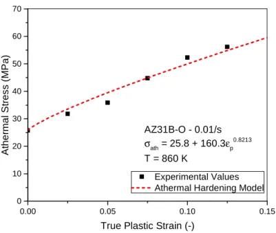
As stated by its name, the athermal stress S_VRW corresponds to the part of the overall stress which is considered independent to the temperature. It is generally generated by the presence of inherent and conditional long range-obstacles [10]. The inherent obstacles (Fisher’s SRO [10, 23] or cutting APBs [10, 24]) are directly linked to the chemical composition of the metal and the conditional obstacles to the level of density of dislocations (cutting attractive junctions or long-range stresses). These last obstacles lead technically to thermo-activated mechanisms but the energies involved along such long ranges (grains size) are very important. Therefore the thermal sensitivities are so small that the mechanisms generated by the conditional long-range obstacles are supposed athermal.

As for the thermal stress, S_VRW is composed of an initial effective stress e_V and of a hardening internal part corresponding respectively to the inherent and conditional contribution of the long range-obstacles [10]. The conditional part of the athermal stress is generally neglected in FCC and BCC metals (the internal thermal stress of this last being considered temperature independent) but is present in other lattice structure such as HCP. An AZ31B-O magnesium alloy is taken as an example (Figure 5).

-5 -4 -3 -2 -1 0 1 2 3 4 5 6 7 0.6 0.8 1.0 1.2 1.4 1.6 1.8 2.0 N o rm a liz e d I s o th e rm a l E ff e c ti v e S tr e s s ( -)

log₁₀(True Strain Rate)

g₀ = 1 g₀ = 0.5 g₀ = 0,2 g₀ = 0.1 g₀ = 0.06

25

Figure 5 - Example of athermal stress presenting a hardening phenomenon due to long range interaction (Mg alloy AZ31B-O)

Strain rate sensitivity of internal stress and viscous drag effect

The evolution of the density of dislocations represents the strain history of the metal. If only the density of mobile dislocations is considered, the history will be identical whatever the strain rate because the statistical mean path of propagation of mobile dislocations stays the same for any value of strain. However, if the density of stored dislocations is taken into consideration, the impact of the strain rate on the internal stress can be important [25] (depending on the density of initial dislocations and amplitude of slip plane activation stress).

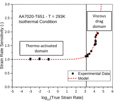
Consequently, FCC metallic materials present generally a positive strain rate sensitivity of the strain hardening [26, 27] (Figure 6) (contrary to the BCC metals for which it is null). However, this sensitivity is not always monotonous. Indeed, phenomenon such as dynamical strain ageing (DSA) can be encountered in metallic alloys. DSA effect causes a negative strain rate sensitivity due to the presence of specific precipitates preventing a smooth motion of the dislocations in their neighborhood [28, 29]. Many dislocations are therefore stacked in a small space causing a high rate of annihilation which increases with the strain rate.

At high strain rates, viscous drag mechanisms (see Appendix D for detailed information) start to be preponderant on the thermo-activated phenomena. The strain rate sensitivity of the stress becomes exponentially important with the rate of deformation [10].

0.00 0.05 0.10 0.15 0 10 20 30 40 50 60 70 Experimental Values Athermal Hardening Model

A th e rm a l S tr e s s ( M P a )

True Plastic Strain (-) AZ31B-O - 0.01/s

σath = 25.8 + 160.3εp 0.8213

26

Figure 6 - Normalized strain rate sensitivity of the internal stress of a AA7020-T651 aluminum alloy

Temperature and strain rate coupling

It has been reported many times in the literature that the thermo-mechanical behavior of metallic materials is greatly dependent on the strain rate. Indeed, the mechanical response of the metals increases with the rate of deformation for a given temperature.

This behavior is mainly caused by the fact that metallic materials do not follow a thermal softening based on a fix reference temperature (generally taken as the melting point). Indeed, the reference temperature, called critical temperature Z , can be lower or higher than the melting point and is function of the strain rate as shown (Eq 1.26 and 1.27) [11, 30, 31]:

Z 8 –>5_{. ln –}7 _!! ˜˜J ( 1.26 )

! 8 _{Q K ( 1.27 )}

With 5₇ the Boltzman constant, . the total energy which is required to overcome the obstacles through thermal activation, ! the athermal transition strain rate, the Burgers’ vector, the dislocation spacing, Q the density of mobile dislocation and K ~10 /• the attempt frequency. The evolution of the critical temperature for different metallic material is shown in Figure 7.

Furthermore, in the case of metallic alloys, a conflict may appear between rates of deformation and kinetics of microstructural changes at very high strain rates (high speed impact …) and a modeling of such phenomena might be needed in some cases.

-5 -4 -3 -2 -1 0 1 2 3 4 5 6 0.0 0.5 1.0 1.5 2.0 2.5 3.0 Experimental Data Model S tr a in R a te S e n s it iv it y ( -)

log₁₀(True Strain Rate) AA7020-T651 - T = 293K Isothermal Condition Thermo-activated domain Viscous drag domain

27

Figure 7 - Theoretical evolution of the critical temperature with the strain rate for several metals

Microstructural changes

Most of metals and metallic alloys presents microstructural changes with the temperature. The only possible change for pure metals is the variation of the grain size but it is much more complex in the cases of multiphasic alloys. Indeed, the thermodynamic equilibrium of the different phases is temperature dependent and these lasts interact between each other. This lead to phenomena such as dissolution or precipitation of phases in a dominant matrix (for instance, the MgZn2 precipitates in the

AA7020 aluminum alloys follow a dissolution process in the aluminum matrix around 490 K [32, 33] (Figure 8)). Besides, the specificities and amount of the phases present in the matrix, condition the mechanical behavior because of their huge impact on the generation and motion of dislocations. Furthermore, for each metallic alloy, many phases can exist outside of the thermodynamic equilibrium: the metastable phases and can be computed using different dedicated software. The Figure 8, shows the evolution of the calorific ratio [34, 35] which consists into the normalized isothermal thermal stress at a given temperature and strain rate (here at room temperature).

-5 -4 -3 -2 -1 0 1 2 3 4 5 6 7 0 2000 4000 6000 8000 10000 C ri ti c a l T e m p e ra tu re ( K )

log₁₀(True Strain Rate) Cua1 AA7020-T651 Mo AZ31B-O 36NiCrMo16 Ti-6Al-4V

28

Figure 8 - Normalized evolution of the thermal stress (isothermal condition) with the temperature in quasi-static and dynamic conditions of the AA7020-T651 aluminum alloy

The two main phenomena which can lead to a significant change in the mechanical behavior are the dissolution of a phase or the precipitation of a phase. The dissolution causes a sudden drop of the stress due to the annihilation of the dislocations around these phases. The precipitation phenomenon leads to a sudden jump of the stress due to the appearing of phases with hardening potential (such as some high strength steels or nickel-based alloys [36-38]).

To fully understand the thermo-mechanic behavior of a metallic alloy over a wide range of temperature, its phase composition has to be investigated and eventually modeled.

Strain mechanisms in amorphous polymers

Polymer materials can be sorted in two categories: amorphous or semi-crystalline. Amorphous polymers are assumed composed of a unique phase of randomly assembled molecule chains. The semi-crystalline polymers are bi-phasic structures, one is amorphous (as for the previous category) and the other is crystalline (the molecule are sorted in a lattice structure in which slips and strain hardening occurs). In this work, only assumed amorphous polymers are studied (Polyimide and epoxy resin). Therefore, only strain mechanisms related to amorphous polymers are explained in this section of the manuscript.

Structure of amorphous polymers

The amorphous polymers do not have an ordered structure as other types of materials possessing a crystalline microstructure [4, 39]. 0 100 200 300 400 500 600 700 800 900 0.0 0.5 1.0 1.5 2.0 Al-Fe-Mn-Si Experimental Data 0.01 /s Experimental Data 2000 /s Johnson-Cook Model Arrhenius law Molinari-Clifton C a lo ri fi c R a ti o ( -) Temperature (K) AA7020-T651 Isothermal Condition ε_p = 0,10 MgZn₂ + Al₆Mn

29

The main concept to be retained concerning the structure of an amorphous polymer is the molecular chain (see Figure 9). An elementary segment [AB] is an element of the macromolecular skeleton containing a single rotatable link and is characterized by its length @ as well as by the angle Θ which it makes with the adjacent elementary segments [BC]; these two quantities being considered as constant. A polymer molecular chain is a succession of elementary segments (which may be different) and have branches. This chain is characterized by various properties such as the molar mass D or its tortuosity.

Figure 9 - Schematic representation of a polymer chain

Random coil

The tortuosity of a molecular chain arises from the probability that an elementary segment is in a trans-left + or - conformation. At each node of elementary segments, the main skeleton of the chain takes the direction imposed by the configuration defined by the following segment (trans = locally straight chain). The end result is a string in the form of a random coil.

The average distance between the ends can easily be calculated by calculating the modulus of the vector OM (Figure 10) (Eq 1.28) [2, 4, 39, 40]:

p² 8 q©Dr 8 ª}

«

¬ ( 1.28 )

With ai the length of the yRW elementary segment and N the number of elementary segments in the

molecular chain. If one considers a molecule at rest (isotropic), for a sufficiently long chain, the sum of scalar products ai.aj vanishes and one can then write Eq 1.29:

p² 8 q©Dr 8 }

«

30

Figure 10 - Schematic representation of the random coil in an amorphous polymer.

If @ characterizes the average length of an elementary segment, one can write Eq 1.30:

p² 8 @² ( 1.30 )

Note that the average distance of the two ends is proportional to the square root of the "deployed" length of the chain.

It is then possible to define the characteristic ratio _~ of the chain defining a quantity closer to reality (Eq 1.31):

~8 lim_«→~žp²_@²¡ ( 1.31 )

The lower the _~, the more compact the statistic ball will be, indicating a great tortuosity of the chain (generally between 1 and 20).

Chain entanglement

When the chains become too long (usually corresponding to a critical molar mass D of several kg / mol), the macromolecules are assembled into a structure which has a very important influence on the thermomechanical behavior of the material [4, 41, 42]. This critical molar mass defines the beginning of a critical entanglement of the polymer molecules [43, 44].

31

(a)

(b)

(c)

Figure 11 - Evolution with the molecular mass of (a) the viscosity, (b) the rigidity and (c) the energy of propagation of the chains [4]

32 - The viscosity for the melted state ° increases much more rapidly with the molar mass beyond

this critical molar mass (Figure 11.a).

- The modulus of elasticity (at a temperature above Z_*) also increases much more rapidly beyond the critical molar mass and tends towards a finite value (Figure 11.b).

- The propagation energy . (critical rate of restitution of the elastic energy) exhibits the same tendency as the modulus of elasticity and tends towards a finite . value (Figure 11.c).

These large increases in mechanical magnitudes are mainly due to the multiplication of intermolecular interactions (increase in cohesion energy) caused by the entanglement of molecules (Debye interactions, London, Hydrogen bonds, etc.). Indeed, the longer the molecules, the more they create links with other molecules, so that they can all become linked to one another (extreme case causing infinite viscosity). In an intermediate case, it is easy to see that the molecules thus entangled have more difficulty to move by crawling than weakly bound molecules leading to a higher viscosity. In the end, this leads to a greater cohesion of the molecules between them, leading to an increase in the modulus of elasticity and toughness of the material (through the increase of the propagation energy .).

Temperature of glass transition

The glass transition temperature Z marks the transition from a thermodynamic state of equilibrium to an unbalanced state (transition from glassy state to rubber state). This is the vitrification state of the polymer [4, 40, 45].

This condition occurs when the cooling of a polymer material is too fast in response to the rate of conformational changes imposed by thermodynamics. The chains thus remain in the configuration which they had just before the cooling. This phenomenon can be compared with the quenching of metals which pass to a metastable state outside the thermodynamic equilibrium by retaining the crystallographic structure which they had at high temperature. The slower the polymer was cooled, the closer its structure was to thermodynamic equilibrium [46].

One can define four temperature domains defining the evolution of the molecular structure without thermodynamic equilibrium [4, 46]:

- If Z { Z , the polymer reaches very quickly thermodynamic equilibrium.

- If Z { Z { Z > ±Z, (±Z corresponds to a few tens of degrees) this domain is called "annealing". The polymer may reach thermodynamic equilibrium after a specific duration.

- If Z > ±Z { Z { Z_\ , this domain is called "physical aging". The structure of the polymer evolves but will never reach the thermodynamic equilibrium (even over very long durations).

33

It is important to know that the glass transition temperature is a very difficult quantity to evaluate experimentally because it depends on many parameters such as cooling rate and measurement frequency (to not miss the transition of thermodynamic behavior). This is why the values found in literature are those measured under industrial conditions so that they are relevant (in most cases) under the conditions of use of engineers and researchers.

The value of Z strongly depends on the strength of cohesion between the chains (intermolecular interactions), the static rigidity of the material and on the density of patella (particularly in presence of aromatic cycles). However, the influence of these quantities may also greatly varies with the level of entanglement of the chains, therefore, the molecular mass plays also a major role in the value of Z .

Physical signification of the yield stress in amorphous polymers

The movement of the molecular chains is induced by a phenomenon of crawling of the latter. The intensity of this phenomenon increases with the rise in temperature. To understand its origin, we must consider the different conformations of the secondary groups around the axis of the main skeleton of the macromolecule (representation of Newman). These conformations are defined as a function of the steric hindrance of the secondary groups [4, 40].

In general, the conformation trans (0°) is the most thermodynamically stable contrary to the left conformations (± 120°). Indeed, the energy is then the most important. The energy necessary to stabilize this conformation is therefore the lowest. Consequently, the energy necessary to achieve a conformational jump increases with the gap of this activation energy (Figure 12). However, raising the temperature makes it possible to increase the probability of a conformation jump and is defined by the relation (Eq 1.32) [39, 42]:

¤ 8 =J ²+ ( 1.32 )

With ³ the energy to be crossed to accomplish the conformation jump, O the perfect gas constant and Z the absolute temperature (K).

It is noted that if { OZ, the jumps are rare events characterizing a rigid chain. However, if z OZ, the jumps have a high probability and the conformational changes are numerous then producing significant motions in the molecular chain and then causing its breakdown.

34

Figure 12 - Potential energy of secondary groups according to their spatial conformation [4]

There are several critical temperatures for each type of polymer molecules defining the transition from a low probability of conformation jump to a high probability because not all conformation sites necessarily have the same secondary group configuration.

These temperatures are called the transition temperatures Z_\, Z_], … and correspond in general to the secondary relaxation mechanisms of the following groups (A, B and C) (see Figure 13):

35

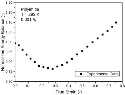
Another phenomenon may be responsible for the movement of the polymer chains, it is the slipping of these chains induced by an external stress (see Eyring theory in the next section about the yield stress). Another characteristic aspect of amorphous polymer can be enounced: the free volume a [47-49]. It corresponds to the volume of the polymer which is not occupied by the chain segments (occupied volume a ) and is consequently composed of voids. The free volume increases linearly with the temperature up to the glass transition temperature Z (temperature of activation for jumps of full chain segments) above which its sensitivity is much stronger (Figure 14). The higher the free volume is, the easier the flow will be. Therefore, at high temperature (above Z ), the yield stress is much smaller than at lower temperature. At a given temperature Z, the fraction of free volume %qZr can be written by Eq 1.33.

%qZr 8_{a o a}a ( 1.33 )

Figure 14 - Evolution of the free and occupied volume with the temperature

Yield stress

The theory developed by Eyring aims to model yield stress [50, 51] . This one is based on the state transition theory. This theory makes possible to model all the thermo-activated phenomena in amorphous polymers. The primary concept consists in the jumps of the segments of the macromolecules from one configuration to another (causing the macromolecule to break). The energy provided by a constraint will allow such jumps. It is assumed that such phenomena start when the stress reaches the

36

flow constraint (even if it is a simplification because other phenomena exist such as adiabatic heating, expansion effects, etc.). Eyring posed three hypotheses:

- In the absence of stress, the ends of the chains of the macromolecules are in a state of thermodynamic equilibrium.

- The deformation of the polymer materials involves the displacement of the chain segments from one thermodynamic state of equilibrium to another.

- The displacement of the polymer chain segments follows a stochastic process. The existence of energy barriers is due to the presence of neighboring polymer chains.

The basic deformation process can be either intermolecular (chain slippage) or intramolecular (chain conformation change). In the absence of stress, the system is in thermodynamic equilibrium and the chain segments move with an oscillation frequency F between the equilibrium positions (Eq 1.34):

F 8 F =J ´&iµ+ ( 1.34 )

With F the fundamental vibration frequency of the chains, Δ0 the activation energy required for molecular displacement, Z the temperature and 5_c the Boltzmann constant. It is assumed that the applied stress σ is responsible for the variation of a symmetrical offset of the activation energy Δ0. Indeed, under constraint, the frequency of conformal jumps increases in the direction of application of the latter. The activation energy thus tends to decrease in this direction by an amount corresponding to the work performed by the displacement of the chains by sliding. This work is expressed by the following expression (Eq 1.35):

¶ 8Sa₂ ( 1.35 )

With a an activation volume (or Eyring volume) representing the volume in which a polymer chain must be able to move to activate the flow. The factor 1/2 is explained by the presence of two chains for each equilibrium position. Whenever an equilibrium position changes, two polymer chains will move. The frequency of the flow F is given by the following expression (Eq 1.36):

F = F =J ´&iµ+· (X

iµ+ ( 1.36 )

Symmetrically, the probability of molecular change in the opposite direction to the direction of stress application decreases. The flow frequency F_c in this backward direction is expressed by the following expression (Eq 1.37):

Fc = F =J ´&iµ+J (X

iµ+ ( 1.37 )

The rate of deformation of a polymer chain being proportional to the difference of the two frequencies

37 ! ∝ F > Fc 8 F =J ´&iµ+ž= (X iµ+> =J (Xiµ+¡ ( 1.38 ) ! 8 ! =J ´&iµ+sinh – Sa 25cZ˜ ( 1.39 )

With the consideration of the limited expansion of the first order, one can write the flow constraint (Eqs 1.40 and 1.41) with the following expression corresponding to the linear Ree-Eyring model [50, 51]:

sinhJ _{» 8 ln 2» ( 1.40 )}

SY82Δ0_{a o}25_{a ln –}cZ 2 !_{! ˜} ( 1.41 ) The effect of the hydrostatic pressure on the amorphous polymer can be implemented in the Ree-Eyring model by simply writing (Eq 1.42):

! = ! =J´&J(X·¼½iµ+ ( 1.42 )

With ¾ the hydrostatic pressure and Ω = a the activation volume under pressure ( is a coefficient modeling the sensitivity of the polymer to pressure).

Strain softening and relaxation of the chains

After yielding, the polymer presents irreversible microstructural changes which can be interpreted as an increase of the internal entropy of the material. Indeed, once the molecules start to slip, the complexity of the chain network can be observed. On one hand, a strong friction, influenced by the local state of stress between the chains, increases the strength of the material with the strain. On the other hand, the chains are not yet in tension and an important freedom of motion of the chain segments is present, leading to a decrease of the resistance of the polymer [52, 53] (depending on the entanglement, the length and the tortuosity of the chains [54]). The strain softening can be seen as the slow extension of the chain fragments (Figure 15) [2]. This relative free motion of the chains lasts until a majority of those chains starts to be locally strained due to excessive tension, causing the hyperelasticity phenomenon.

38

Figure 15 - Illustration of mechanisms and resultant stress of strain softening phenomenon

The relaxation of chains is a phenomenon which can be observed when the tension on a chain segment is locally released. The hyperelasticity being a reversible phenomenon, the chain segment springs back to an energetically optimal position in the chain network depending on the available local free volume [52]. The corresponding time of this phenomenon is called the characteristic relaxation time of the polymer [2].

Hyperelasticity phenomenon

The hyperelasticity phenomenon is caused by the overall resistance to the applied strain of the polymer chains network and results in a back stress [2, 55]. The higher the strain is, the higher the back stress will become. This increase of the hyperelastic stress can be microscopically explained by the alignment of all the chains, which can be considered as strings, in the direction of the highest local equivalent strain. Therefore, at macroscopic level, the back stress will be highly dependent on the state of stress which will condition the alignment behavior of the chains. Thermodynamically speaking, hyperelasticity is associated with a decrease in the entropy of chain configuration during the extension of the material and an increase during the compression (Figure 16).

The back stress is generally computed from an energy density of deformation function ¶. Two hypotheses are made [56]:

- The strain energy density is a function of the strain gradient.

39

The energy density of deformation can be written (by considering the two first principles of thermodynamics) with the following expression (Eq 1.43):

¶¿jjjjj 8 CÀÁ _{2 nZp¿}jjjjjÂu o 26Zp nÀÁ jjjjj u ÀÁ ( 1.43 )

With jjjjj the strain tensor of Green-Lagrange and 6 and C are elastic constants of the hyperelastic _ÀÁ material.

Figure 16 - Illustration of hyperelasticity phenomenon and resultant stress

Constitutive modeling of mechanical behavior

Constitutive of mechanical behavior

The necessity of using constitutive mechanical law is of the upmost importance. There are several analytical methods to address the problems of mechanics. The first historically uses the concept of force while newer methods use the energy or power concepts. This last is the most practical to use (since the force can be directly measured through force cell) for modeling of complex mechanical systems and is becoming one on which is based the finite element method widely used by simulation softwares. The virtual power is expressed (Eq 1.44) in terms of the velocity field b and force à which may correspond to any type of action (internal or external). For a system Σ [4, 57]:

¾ 8 € Ã. b E

Å

( 1.44 ) With E an infinitesimal fraction of the system Σ.

The action which may be encountered:

- External ¾ if there is an exchange of energy with the outer part of Σ (contact or remote)

- Interior ¾ if the action concerns interactions between particles within the system. The power of deformation is opposed to the power of internal actions and is expressed as follow (Eq 1.45):

40

¾^ 8 >¾ _{( 1.45 )}

- The acceleration actions ¾_V corresponds to the volumetric field >Q/ with Q the density and / the acceleration.

Assuming that there are at any time and for any movement a Galilean space in which the sum of the virtual power related to Σ vanishes (especially when considering eulerian tensor systems):

¾ o ¾ o ¾V= 0 ( 1.46 )

The principle of virtual power is stated entirely on equation (Eq 1.46).

If we consider the eulerian Cauchy strain tensor k is considered (Eq 1.47), the tensor of the associated constraints, also eulerian, is called Cauchy stress tensor Sj.

k = 1_{2 n ∇}jjjjb + ∇kbu + ( 1.47 )

Assuming that the system Σ is subjected to forces only on a part of ÇΣ_È and the displacements on the complementary part ÇΣ_X to be zero. The motion is considered kinetically admissible to zero. We then find (Eq 1.48):

¾^ = € Sj. k Å

a ( 1.48 )

With a an infinitesimal volume fraction of the system Σ.

By considering the strength of external actions, the forces of volume actions % (always related to the density Q) have to be taken into account separately from the surface forces É exerted on ÇΣ_È. If coupled masses are neglected, we get Eqs 1.49 and 1.50:

¾ = € Q%. b a Å + € É. b ‹ ŒÅÊ ( 1.49 ) With: ¾V= − € Q/. b a Å ( 1.50 ) We can then write the full form of the virtual power principle (Eq 1.51) [58, 59]:

€ Sj. k Å a − •€ Q%. b a Å + € É. b ‹ ŒÅÊ ¢ + € Q/. b a Å = 0 ( 1.51 )

Considering the expression of the Cauchy strain tensor k and the symmetry of Sj, the formulation becomes Eq 1.52:

41 € Sj: ∇kb a > € Qq% > /r. b a > € É. b ‹ = 0, ∀b ŒÅÊ Å Å ( 1.52 ) By integration by part of the first integral and using the Ostrogradski relationship, we get Eq 1.53:

€ ªÇS_{Ç» o Qq% > / r¬ b}Ì Ì a > € SÌG bÌ ‹ ŒÅÊ Å o € É bÌ ‹ = 0 ŒÅÊ ( 1.53 ) Virtual movements are random, if any b are taken in Σ and if b is considered null on ÇΣ_È, then the first integral should be zero regardless of b (Eq 1.54):

ÇSÌ

Ç» o Qq% > / r = 0 ( 1.54 )

Eq 1.38 is also called the indefinite equations of motion (3 in number) or of equilibrium if / is zero. A more practical expression (Eq 1.55) [59]:

ybSj o Qq% > /r = 0 ( 1.55 )

The virtual movement being always random, a second equality comes from both remaining surface integrals on ÇΣ_È (Eq 1.56):

SÌG = É or SjG = É ( 1.56 )

These three equations (given by Eq 1.39) from the latter formulation give the boundary conditions of the principle of virtual power and raise the unknowns of the problem.

These formulations allow the determination of the value of the Cauchy stress tensor Sj for all the system according to the deformation and also to be able to know the power levels and thus the energy of the system.

The discretization in small elements is easy to do and allows very precise computations across complex systems. However, the calculation time is very long. For this reason, the finite element method and diverse algorithms have been created (size and shape of the surface elements or discretization volume for example). Conversely, the finite element method can be used to solve other problems from thermal to magnetic ones (with integral formulations from other principles than the one of virtual power). A summary of all the equations available after processing the principle of virtual power can be found in Table 1 [4].