Comparison of managed and unmanaged forest stands in France based on diameter diversity and spatial forest structure indices

HAL Id: hal-02602149

https://hal.inrae.fr/hal-02602149

HAL is a multi-disciplinary open access

archive for the deposit and dissemination of sci-entific research documents, whether they are pub-lished or not. The documents may come from teaching and research institutions in France or abroad, or from public or private research centers.

L’archive ouverte pluridisciplinaire HAL, est destinée au dépôt et à la diffusion de documents scientifiques de niveau recherche, publiés ou non, émanant des établissements d’enseignement et de recherche français ou étrangers, des laboratoires publics ou privés.

France based on diameter diversity and spatial forest

structure indices

A. Gillespie

To cite this version:

A. Gillespie. Comparison of managed and unmanaged forest stands in France based on diameter diversity and spatial forest structure indices. Environmental Sciences. 2014. �hal-02602149�

- 1 -

Master Thesis

Presented by

Alexandra GILLESPIE

In order to obtain the diploma of

MSc Sustainable Tropical Forestry

Subject :

Comparison of managed and unmanaged forest stands in

France based on diameter diversity and spatial forest

structure indices

Defended publically on the 19

of December 2014

at AgroParisTech,

Montpellier Center

In front of the following jury :

M. Yoan PAILLET

Supervisor

Dr. Ghislain VIEILLEDENT

Researcher, CIRAD

ACKNOWLEDGEMENT

I would first like to thank my master thesis supervisor, Yoan Paillet, for his help and advice during my time with Irstea. I would also like to thank Philippe Balandier for his ideas and opinions. Sylvie LeRoux provided excellent administrative support and I thank her for all her help with travel arrangements and reimbursements as well as Jean-Pascal Barrau for dealing with French administration questions.

I would also like to extend my gratitude to Christian Rippert, Carl Molliard, Fanny Le Bagousse and Philippe Janssen for their assistance in the field.

Thomas Perot should also be mentioned for his help with spatial point processes and Anne for her ingenious help with R loops.

I am grateful to Irstea, the Irstea team and the CONSPIIRE project for having given me the opportunity to work on this subject and assist various events and conferences at their behest. Finally, I would like to thank my AgroParistech tutor, Raphaël Manlay, for being available to respond to any questions I might have and for all his support and help in organizing the thesis defense.

FOREWORD

The six-month internship took place within the Institut de recherche en sciences et technologies pour l’environnement et l’agriculture (Irstea), a French research body with more than 30 years’ experience in studying major issues including: a responsible agriculture, the sustainable land management of territories, water management and associated risks, droughts, floods, the study of complex ecosystems and of biodiversity and its relationship with human activity. The multi-disciplinary research conducted supports public policies and works in partnership with regional authorities and socio-economic entities (Irstea, 2014).

The project I worked for during my six-month internship is a research project called “Construction and potential indicator value of multi-scale forest structure indices (CONSPIIRE)”. It aims at increasing the knowledge on the link between forest structure and biodiversity and improving the indicator value of forest structure indices. Funded by Irstea, the project started in late 2013 for a duration of two years and is a collaboration between researchers in the Nogent-sur Vernisson, Grenoble and Aix-en-Provence Irstea centers.

- 5 -

ABSTRACT

Nineteen forest structure indices were compiled and compared to test how they differ in their characterization of managed and unmanaged stands in French forests. Thirteen distance-independent diameter diversity forest structure indices and six distance-dependent indices were used to characterize and compare 257 managed and unmanaged stands in 20 lowland and mountain sites part of a national stand network in France. Most spatially-implicit diameter diversity indices characterized unmanaged lowland forest stands as more complex to a certain degree with significantly superior basal areas, variability, diversity, dominance and inequality than their managed counterparts. Management differences were not as evident in the case of mountain forest sites due to their uneven-aged long rotation cycles. Distance-dependent indices were unable to provide clear results as to the spatial pattern of stands, due to the small fixed area plot size. Additional neighbor measurements as part of the larger angle-count method could help characterize the stands spatially. Indices with the best discriminant ability and reliability that can be used to monitor the forest structure of these stands and the shift from forest management to natural forest development include the basal area, the coefficient of variation of the diameter, the Shannon index, and the Gini coefficient.

RESUME

Dix-neuf indices de structure forestière furent compilés et comparés pour déterminer en quoi ils diffèrent dans leur description de placettes exploitées et non-exploitées françaises. Treize indices de diamètre et six indices spatiaux quantifièrent la structure de 257 placettes forestières exploitées et non-exploitées réparties sur 20 massifs de plaines et de montagnes dans un réseau national de placettes en France. La majorité des indices de diamètre caractérisèrent les zones non-exploitées en plaine avec des surfaces terrières plus élevées, et des diamètres plus variables, diverses, dominants, et inégaux, que les forêts exploitées. En montagne, les écarts étaient moins significatifs à cause de la structure équienne et des rotations à long terme des placettes exploitées. Pour la structure spatiale des placettes, les résultats obtenus ne furent pas concluants car la dimension des placettes à rayon fixe était trop petite. La mesure d’arbres voisins supplémentaires dans la mesure d’arbres à angle fixe aiderait à caractériser les placettes spatialement. Les indices les mieux capables de discerner entre placettes exploitées et non-exploitées peuvent cerner leur structure forestière et leur passage d’une forêt exploitée à une forêt naturelle – ceux-ci sont : la surface terrière, le coefficient de variation du diamètre, l’indice de Shannon et l’indice de Gini.

TABLE OF CONTENTS

A

... 3

F

... 4

A

... 5

R

... 5

1.

I

... 9

2.

M

... 12

2.1. Description of the study sites 12 2.2. Data collection 14 2.3. Description of the indices 14 2.3.1. Distance-independent indices ... 21

2.3.2. Distance-dependent indices ... 22

2.3.3. Combination indices ... 23

2.4. Calculation of the indices 23 2.4.1. Distance-independent indices ... 23

2.4.2. Distance-dependent indices and combination indices... 24

2.5. Data analysis 25

3.

R

... 28

3.1.1. Distance-independent indices ... 31

3.1.2. Distance-dependent indices ... 32

3.1.3. Combination indices ... 33

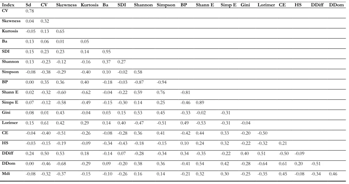
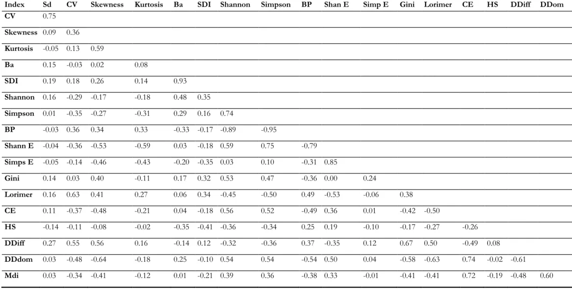
3.1.4. Correlations between indices ... 34

4.

D

... 35

indices 35

4.2. Differences between lowland and mountain sites 35

4.3. Indices that rejected the null hypothesis 36

- 7 -

5.

C

... 39

6.

R

... 40

7.

L

... 48

8.

T

... 49

9.

T

... 50

10.

A

... 51

T

A

... 51

Annex 1 – Description of CONSPIIRE project 52

Annex 2 – Summary data per forest stand 57

Annex 3 – GNB Secondary protocol 71

Annex 4 – Systematic Review Protocol 75

Annex 5 – R script: Calculation of diameter differentiation, dominance and mean directional

index 78

Annex 6 – R script: Calculation of 16 other indices 87

Annex 7 – R script: Linear mixed model analysis of indices 95 Annex 8 – Results of Tests in R: Tukey multiple comparison of means and Analysis of variance115

Annex 9 – Correlation Tables 120

9

-1. INTRODUCTION

The importance of forest ecosystems and their management have risen to the public attention in the past few decades since the establishment of the Convention on Biological Diversity (CBD) in 1992. While tropical forests are experiencing high rates of deforestation, the area of temperate forests has broadly stabilized, with a slight increase in Europe (CBD, 2014a, CBD, 2014b, United Nations Environment Programme et al., 2009).

In mainland France, forests cover about 30% of the territory with 17.6 million hectares, out of which one quarter are public and the rest are private (Ministère de l'écologie, 2015). France has put the accent on biodiversity and its preservation with its adherence to the CBD, its own national policies towards protecting the environment under its National Strategy for Biodiversity adopted in 2004 and the adoption of the Grenelle Environment framework of 2007, which includes forest logging and biodiversity (Gosselin & Laroussinie, 2004). The French state monitors whether it has met its biodiversity and forestry targets mainly via the National Observatory of Biodiversity (ONB) indicators, which focus on dead wood and forest surfaces with multi-stories (ONB, 2011). At a European level, six criteria are used for sustainable forest management, including the promotion of forests’ biological diversity, health and vitality and productive functions (Forest Europe, 2014).

French forest management along with forest and biodiversity levels has also been monitored via the comparison of the structure of managed (i.e. exploited) and unmanaged (i.e. forest reserves) stands (Paillet et al., 2010). Natural dynamics, lacking in anthropogenic pressures,tend to result in more complex forest structures (Hett & Loucks, 1976, Paillet et al., 2010), whereas management decisions can lead to structures that are more uniform (Lähde et al., 1999). Forest structure can thus be a proxy to biodiversity since a positive correlation has been found between structural variables and richness (Tews et al., 2004).

Forest structure is an important element of biodiversity, and more precisely forest stand biodiversity (LeMay & Staudhammer, 2005, MacArthur & MacArthur, 1961). Stands with a variation of tree sizes tend to have higher biodiversity and structural diversity, which is why tree size is one of the most significant indicators of forest diversity (Buongiorno et al., 1994, MacArthur & MacArthur, 1961).

Since forest stands tend to have multiple dimensions, it is sometimes challenging to describe forest structure adequately. McElhinny (2002) defined forest structure as a polysemic term divided into three different attribute groupings: structure, function and composition, whereby structure means the spatial arrangement between components of an ecosystem, function stands for ecological processes and composition refers to the variety and identity of elements (McElhinny, 2002). Stand structure includes vertical structure (e.g. understory trees, number of tree layers), defined as the differentiation of layers between ground and the canopy (Bourgeron, 1983, Maltamo et al., 2005, Zimble et al., 2003), and horizontal structures (e.g. spatial pattern of trees, gaps), referring to the diameter size distribution of either individual or trees species within one community (Davis & Johnson, 1987, Maltamo et al., 2005, Zimble et al., 2003).

According to Pretzsch (2009), the most important aspects of stand structure are the horizontal distribution configuration of trees, density of the stand, the differentiation of sizes, and species intermingling since they affect habitats, growth processes, and the stability of the ecosystems. Since the most common elements of stand structure measured in France include (but is not limited to) live tree diameter and geographical position (Bruciamacchie et al., 2007, Tomppo et al., 2010), this study focuses on these elements of horizontal structure and defines stand structure as the distribution of live tree sizes within a forest stand (Newton, 2007).

Indices are often used for describing changes in the structure of a forest stand or for stand comparison since they compress multiple dimensions concisely into a single number (Magurran, 2004, McElhinny et al., 2005). Measurements of a few structural attributes such as live-tree sizes

or horizontal variation in canopy density can help estimate other structural conditions and the ecological state of a forest (Spies, 1998). Structural complexity can be a surrogate for the potential of forest stands for biodiversity, and as such differentiating stands with different structural states can be useful as metrics and indices but also provide clues as to the driving structure of ecological processes (Peck et al., 2013). Structural complexity can be defined as the spatial horizontal and vertical arrangement of plant dimensions (Zenner, 2000).

The majority of comparative studies in the past have focused on classical old growth forest structure measures such as basal area, large trees and dead wood for the characterization of unmanaged old growth stands and their comparison to managed stands (Christensen & Emborg, 1996, McElhinny, 2002, Nilsson & Baranowski, 1997, Pernot et al., 2013). In terms of other measures or indices that can be used, there is no single forest structure index preferred over the others, so selecting an appropriate index for the comparison of stands can be difficult (McElhinny et al., 2005). Authors differ in their preference of stand elements (e.g. diameter, height, tree spacing) or structural attributes1_{, construction of the index as well as the use of spatial patterns} (LeMay & Staudhammer, 2005, McElhinny, 2002).

Authors that have applied structural indices to forest stands have made a distinction between plantations, even-aged, managed stands and uneven-aged, semi-natural and natural (or primary) forests stands (Commarmot et al., 2005, Ex & Smith, 2013, Lexerød & Eid, 2006, Marinšek & Dlaci, 2011, Mason et al., 2007, Sterba, 2008, Sterba & Zingg, 2006, Szmyt, 2012, Uuttera et al., 2000, Vencurik et al., 2012). One case-study by Bilek et al. (2011) in Central Bohemia compared spatially-implicit (i.e. distance-independent) and spatially-explicit (i.e. distance-dependent) indices in managed and unmanaged stands over time. Nevertheless, a large scale comparative investigation of forest structural complexities through a broad national stand network has not been attempted to date (to this author’s knowledge) and can help represent the structural variability of French temperate forests between managed and unmanaged stands (Clark, 2007, Wagner et al., 2010).

The six-month internship that led to the writing of this master thesis took place within the Institut de recherche en sciences et technologies pour l’environnement et l’agriculture (Irstea). The Irstea project that funded the internship is called the “Construction and indicator value of multi-scale forest structural indices” (CONSPIIRE) project and aims at finding a relevant indicator value of forest structure indices and its link to biodiversity (Irstea, 2015). The research will feed into the ongoing efforts to improve the Indicators of Sustainable French Forests Management and the European reporting on the state of forests coordinated by Forest Europe (see Annex 1 for more details on the CONSPIIRE project).

The internship focused purely on horizontal and spatial forest structure indices, because, as was argued above, they can be a reliable proxy to biodiversity and management differences. The internship represents a first step towards increasing the knowledge on forest structure indices already in use in the literature and their usefulness in comparing management structures. The first internship objective was to conduct a literature review of forest structure indices and the subsequent selection of appropriate indices for a comparison of managed and unmanaged stands. The selected indices were narrowed down based on the literature review on diameter diversity and spatial forest structure indices at the stand level as well as data availability so that the second aim of the study can be completed.

Once indices have been selected, the second objectives of the study is to calculate the selected indices in order to compare managed and unmanaged stands using pre-existing data. The data for the calculation of the indices stems from data compiled in a French national forest stand network, which included the measurements of live tree diameter and location and further narrowed down the choice of indices. Once calculated, the thesis will investigate which indices can best indicate which diameter diversity and spatial forest structure indices can detect a management difference.

1 _{Stand attributes describe the identity and variety of stand elements, their spatial arrangement or the types}

and rates of ecological processes; common stand attributes are tree diameter at breast height (DBH), standard deviation of DBH, diameter distribution, and basal area (McElhinny et al, 2005).

- 11 -

The study will examine whether managed and unmanaged forest stands differ in a French plot network according to diameter diversity and spatial forest structure indices. The null hypothesis is that there is no significant difference in the forest structure indices selected between managed and unmanaged zones.

The problem statement of the thesis is therefore: how do the forest structure indices selected differ between managed and unmanaged stands? The aim of the thesis is to look at the difference in diameter sizes and spatial patterns characteristics in managed stands where human interventions have influenced forest stands and how these stands differ from unmanaged adjacent plots (for a minimum of 20 years and an average of 50 years) in similar stand conditions2_{. With} the majority of forest structures exploited in Europe at a time or another, forest structures between managed and unmanaged stands would be expected to show a variation ranging from old growth characteristics to forest plantations although unmanaged stands would be expected to have more old growth characteristics (Wolf, 2005). Managed plots can be used as a benchmark or a control since they are the starting point for restored unmanaged plots and how these are progressing to a more natural state (Sterba, 2008).

This study will take place in the Forest Management, Naturality and Biodiversity (GNB, http://gnb.irstea.fr) stand network in France comprising of a total of 20 forests and 257 stands inventoried. Nineteen indices were calculated for the stands in order to gauge which indices can detect a difference in management. In the first part of the study, materials and methods are described which includes the study site description, and details on data collection and data analysis. A short review of index literature and a list of the indices selected for the analysis and details on their calculation is included in this first part. In the second part of the study, the results of the indices are revealed. The last part includes a discussion on the characteristics of managed and unmanaged stands, on the management differences between lowland and mountain stands, and on which indices were able to detect a management difference and can be relevant for future studies. The relevance of the spatial indices and the sampling method used for the study are also discussed.

2 _{For a study on how discontinuing logging activity affects forest structure in French forest reserves, please}

2. MATERIAL AND METHODS

2.1. Description of the study sites

The study uses data gathered as part of the Gestion forestière, Naturalité et Biodiversité (GNB, http://gnb.irstea.fr) forest stand network illustrated in Figure 1. The GNB project began in 2008 in partnership with the National Forest Service (ONF) and the Natural Reserves of France (NR) and aims at evaluating the impact of forest exploitation on biodiversity (Irstea, 2015, Pernot et al., 2013). The network comprises of a total of 20 beech-dominated forest sites, representing around 40% of the total woodland in mainland France (IGN, 2014), including managed and unmanaged areas in controlled site conditions.

Figure 1: Existing GNB forest stand network in metropolitan France as of mid-2014 (Modified from GNB, 2014)

Legend

GNB Forest sites Forest cover

- 13 -

The GNB forest sites were selected according to the following criteria3_:

 Existence of a strict reserve at least 20 years old;

 Forests were also chosen based on their predominant tree species - beech (Fagus sylvatica L.) and oak (Quercus robur L.) were favored for lowland/plain sites (elevation ≤ 800 meters (m)) and fir (Abies alba Mill.) and spruce (Picea abies Karst.) were favored in mountain sites (elevation > 800m).

Table 1: GNB forest sites as of mid-2014

Forest sites MAN

stands UNM stands Average altitude Class of altitude *

Management

type Surface (ha) UNM surfac e (ha)

Anost (ANO) 4 4 686 LOW Even-aged 1,030 68

Auberive (AUB) 12 12 455 LOW Uneven-aged 5 ,580 232 Bois du Parc (BDP) 5 5 183 LOW Even-aged 1,600 45 Chatillon-sur-Seine

(CHS) 4 4 354 LOW Even-aged & uneven-aged 8,900 76 Chizé (CHZ) 12 12 80 LOW Even-aged 4 ,820 2,579 Citeaux (CIT) 6 6 232 LOW Even-aged 3 ,561 47 Combe-Lavaux (CL) 4 4 428 LOW Even-aged 4,056 300 Fontainebleau (FTB) 13 16 132 LOW Even-aged 17 ,072 444 Haut Tuileau (HT) 7 7 164 LOW Even-aged 2 ,567 127

Parroy (PAR) 4 4 272 LOW Even-aged 2,790 161

Rambouillet (RMB) 8 8 168 LOW Even-aged 14,090 115 Verrières (VER) 4 4 173 LOW Even-aged 576 42 Ballons-Comtois

(BC) 8 8 1,013 MON Uneven-aged 2,259 274

Chartreuse (CHA) 5 5 1,278 MON Uneven-aged NA 50

Ecouges (ECO) 5 5 NA MON Uneven-aged NA 248

Engins (ENG) 5 5 1,581 MON Uneven-aged 1, 016 190 Haute Chaîne du

Jura (HCJ) 8 8 816 MON Uneven-aged 7, 989 2,130 Lure (LR) 4 4 1,463 MON Uneven-aged 3,981 553 Ventoux (VTX) 5 5 1,343 MON Uneven-aged 3 ,474 907 Ventron (VEN) 4 4 933 MON Uneven-aged 1, 648 397

Total 127 130 39,282 8,985

* LOW stands for lowland sites and MON for mountain sites; MAN stands for managed stands and UNM for unmanaged stands; NA= Not available.

In order to avoid a possible bias because of site factors (such as biogeographic regions, altitude, slope and soil acidity) between unmanaged and managed stands, the locations of the stands were picked at random with a site-specific constraint to make sure each managed stand had an unmanaged stand equivalent. Managed plots were selected in a radius of 5 kilometers from the forest reserve boundary and included only native tree species. The 257 sites cover a broad array of

stand structural stages ranging from regeneration to old growth stands. Due to field constraints, the final sample of 257 stands is not entirely balanced and comprises of more lowland sites than mountain sites. Most of the unaged forests were located in the mountains whereas the even-aged high forests were located in lowland sites as shown by Table 1. As of mid-2014, the project had inventoried a total of 257 individual stands in 20 forests in lowland/plain and mountain sites (see Figure 1), which are divided into lowland and mountain categories in Table 1.

2.2. Data collection

GNB data were recorded for the 257 stands from 2008 to mid-2014 by Irstea, ONF and NR staff members as well as Irstea interns. The year period for the inventories vary (details of when inventories took place are available in Annex 2).

The GNB protocol followed the national forest evaluation protocol (Bruciamacchie et al., 2007, Paillet et al., In prep) and included diametermeasurements and species documenting of live trees, dead and regenerating trees as well as biodiversity data on seven taxa (vascular flora, bryophytes, mushrooms, beetles, birds, bats and deer) (GNB, 2014).

Relevant measures to the study include diameter at breast height (1.3 m above the ground, dbh) at two different angles and tree locations using a combination of fixed-angle and fixed-area tree-sampling methods (see Figure 2 for an illustration of the two methods). Within a fixed area with a radius of 10 m (314 m²), the dbh of living trees was measured for trees ranging from 7.5 to 20 cm in the plains (7.5 to 30cm in mountain stands). A fixed-angle method was used to inventory living trees over 20 cm in dbh (30 cm in mountains) where trees within a fixed relascopic angle of 2% (3% in mountains) were measured at a maximum distance of 40 m. The Global Positioning System (GPS) coordinates of each stand center were recorded, as well as

the azimuth and distance of each live tree from the center of the stand. The protocol varied in mountains due to rougher conditions. Annex 2

contains summary statistics for each of the 257 stands, including mean dbh, the number of

trees at 40 m, 20 m and 10 m as well as the XY GPS coordinates of each stand.

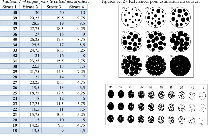
During the internship, a second complementary protocol to the GNB protocol was developed and carried out, available in French in Annex 3. The two-month fieldwork consisted of measuring the height of the five trees with the largest diameters in the 257 stands, the canopy cover of each stand, and the cover of vertical strata of each stand. While the data extracted from the internship fieldwork was not used in the purview of this study, it will be used for future CONSPIIRE work.

2.3. Description of the indices

During the internship, a literature review of forest structure indices has been carried out and 19 forest structure indices were selected at the stand level for the comparison of managed and unmanaged stands. The literature protocol in Annex 4, based on Pullin and Stewart (2006) guidelines for systematic literature reviews, was used to conduct the literature review.

Since there are a myriad of indices in the literature used for analyzing forest stands, reviews can be particularly useful for grouping and selecting indices. Reviews on forest structure indices at the stand level include works from Staudhammer (1999), McElhinny (2002), Pommerening (2002), and LeMay and Staudhammer (2005). These and other authors have grouped indices in various Figure 2: Illustration of the two sampling methods used by GNB

- 15 -

ways. LeMay and Staudhammer (2005) have the following groupings: indices based on tree attributes, indices based on spatial heterogeneity, and a combination of the two. Pommerening (2002 & 2006) classed them in terms of their diversity of tree dimensions; tree species diversity; and tree positions diversity (or spatial distribution), and then further divided them into distance-dependent and distance–indistance-dependent measures. Valbuena et al. (2012) identified four types of distance-independent indices that describe the diversity of tree size classes: adapted species biodiversity indices, adapted species equitability indices, indices based on dispersion estimates of tree size and methods based on descriptors of a histogram’s shape. On the other hand, distance-dependent indices can be divided as tree-level nearest neighbor or competition indices; stand level aggregation or neighborhood indices (Aguirre et al., 2003, Gadow & Hui, 2002, Hui et al., 1998); and second order characteristics (Neumann & Starlinger, 2001, Ni et al., 2014, Pommerening, 2006, Sterba & Zingg, 2006, Szmyt, 2014). Some authors have also developed multi-attribute (or complex) indices and synthetic (or composite) indices which incorporate more than one index (Becagli et al., 2009, Jaehne & Dohrenbusch, 1997, LeMay & Staudhammer, 2006, Pastorella & Paletto, 2013, Staudhammer & LeMay, 2001). Figure 2 provides an overview of the different groups of forest structure indices found within the literature (with the exclusion of the species diversity indices as it is outside the scope of this study).

Figure 3: Overview of the groups of indices by which forest structure is assessed (modified from Pommerening, 2002)

The 19 indices selected for the study were based on the following criteria:

 Appropriateness, mention and use in literature – at least two journal articles on forest structure need to have mentioned the indices;

 Use of diameter, diameter classes and/or location (since this is the data available for the study);

 Resulting in a single index value;

 Ease of calculation as well as access and availability of R scripts and R packages for their calculation;

 At least one index (and a maximum of three indices) per the categories illustrated in Figure 2 was selected – apart from complex and synthetic indices, which lay outside the bounds of this study.

Table 2 gives an overview of the indices used in this study based on the criteria above. The indices have been divided into distance-independent and distance-dependent categories and are

17 -Table 2: Description of indices selected and related R software resources

Index Formula Where Range R package / script

Standard deviation _ 







x

x

N

s

)

(

1

1

i=ith observation in sample N=sample size

stats (R Core Team, 2014)

Coefficient of

variation (%) ( )*100

x s

cv  (2) s=standard deviation x=sample population stats (R Core Team, 2014)

Basal area

4 2 d g

(3) d = tree dbh stats (R Core Team,

2014) Stand density

index SDI = N*(QMD/25.4)1.605 ₍₄₎

QMD= Quadratic mean diameter i= ranges from 1 to N

N = number of trees per hectare

stats (R Core Team, 2014) Shannon index     s j i i p p H 1 ln (5)

pi= proportion of individuals in the ith diameter class,

S= number of size classes

[0; 2.39*] * H’max=ln(S) BiodiversityR (Kindt, 2005) Simpson index Ds=



1 ₍₆₎ pi= relative frequency of number of stems

at each size class [0;11*]

*Dmax=S

BiodiversityR (Kindt, 2005)

Berger-Parker

index DBP=1/max(pi) (7) p= relative frequency of number of stems _{at each size class} [0;1] BiodiversityR (Kindt, ₂₀₀₅₎ Shannon

Evenness EH'/H'_maxH'/lnS (8)

H’=Shannon index H’ max= Max Shannon S= number of size classes

[0;1] BiodiversityR (Kindt, 2005) Simpson Evenness                  11 (₂ ) s s D pi Var E (9) Ds= Simpson index

Var(pi)=variance of abundance pi

[0;1] BiodiversityR (Kindt,

Index Formula Where Range R package / script Gini index

_

_













1

1

2

n

di

di

n

i

G

d= dbh in diameter size class i= rank of a tree in ascending order n=total number of trees

[0;1]

= 0 – equality = 1 – inequality

reldist (Handcock, 2014)

Skewness (11) n= number of sample trees/ plot xi= individual tree dbh,

x

s= standard deviation of tree dbh

< 0 - negatively skewed = 0 - symmetric > 0 - positively skewed moments (Komsta, 2012) Lorimer index L L

X

X

X

M

I







XL= the lower threshold dbh

X0.95 = the 95th percentile of the diameter distribution

< 0.5 - negatively skewed = 0.5 - symmetric > 0.5 - positively skewed

stats (R Core Team, 2014)

Kurtosis (13) n= number of sample trees/ plot xi= individual tree dbh,

x

s= standard deviation of tree dbh

> 3 – leptokurtic = 3 – mesokurtic < 3 – platykurtic moments (Komsta, 2012) Mean directional index (14)        n j ij n j ij i a a R 4 4cos( ) sin( ) 1

aij= angle between i and j points = 0 – square lattice arrangement

> 0 – clustered arrangement Diversity script (Pommerening, indices 2012) Clark Evans index (15) ) (r E observed r R

r ̅observed = observed mean distances between trees

E(r)= mean nearest neighbor distance in stand with completely random tree locations of intensity N/A, whereby:





r

E( )1/2 / (16) A = area of forest stand (m2₎ N = number of trees [0;2.1491] > 1 - regular pattern = 1 - a random pattern < 1 - a clustered pattern spatstat (Baddeley, 20 05)

- 19 -

Index Formula Where Range R package / script

Hopkins-Skellam index          _N i i N i i N i i A 1 1 1  

 (17) ω’i= quadratic distance from sample point to nearest tree

ωi= quadratic distance from tree to nearest neighboring tree

> 1 - aggregated population = 1 - randomly distributed population < 1 - regular population spatstat (Baddeley, 2005) Ripley L function K d _d d L    ) ( ˆ ) ( ˆ (18)      j x i x s x_i x_j d K 0 2 ( ) 1 ) (  (19)  ) 2 2 ( ) (r ab r a b r s     (20) stand λ = density r= distance j x i

x  = distance between tree i and j

s(r) = edge effect correction where a, b are dimensions of the rectangular plot

[0;1] = 0 – random population > 0 – clustering <0 - regularity splancs (Rowlingson, 2014) Dbh Differentiation ) , max( ) , min( 1 j i j i ij DBH DBH DBH DBH T  

(21) DBH = breast height diameter [0;1]

= 0 - No differentiation = 1 - very strong differentiation

Diversity indices script (Pommerening, 2012) Dbh dominance



_

n

U

1

uj = 1, if DBHj ≥ DBHi; otherwise 0

[0;1]

= 0 - No dominance

= 1 - very strong dominance

Diversity indices script (Pommerening, 2012)

21

-2.3.1. Distance-independent indices

The distance independent indices are the following:

2.3.1.1 Simple indices

The standard deviation (Husch et al., 2003) of tree dbh measures the variability in tree dimension, thus is a straightforward attribute to calculate. It has been compared in its usefulness to describe stand structure to more complex attributes and indices (Neumann & Starlinger, 2001).

The coefficient of variation of tree dbh measures size inequality (Hutchings, 1997) – it is the percentage of the arithmetic mean of the standard deviation and is used to compare population samples in relative variability.

Basal area is a useful measure of stand density and competition since it incorporates the number of trees and diameters in a stand. It is calculated by summing the section at 1.30m of each individual tree (Husch et al., 2003).

The stand density index (Reineke, 1933) describes stand density by calculating the quadratic mean diameter and number of stems per unit area. It uses an index tree diameter of 25cm in Europe (10 inches in the U.S.) and a constant b of -1.605, which Reineke (1933) found was consistent with several species and age and site quality independent (Pretzsch & Biber, 2005).

2.3.1.2 Adapted species biodiversity indices

A straightforward way to describe forest complexity would be to just determine the number of size classes in a stand (richness) (Valbuena et al., 2012). The following six indices are based on size classes.

Adapted from the Shannon diversity index for species (Shannon & Weaver, 1949), the Shannon index for diameter classes describes the class richness and relative abundance of every class as well as its rarity by measuring the uncertainty of a tree belonging to a class as a weighted average (Buongiorno et al., 1994, LeMay & Staudhammer, 2005, Pommerening, 2002, Staudhammer, 1999, Valbuena et al., 2012). In this case, the Shannon index has a minimum of zero when all trees are in the same diameter class and a maximum of the logarithm of the total number of classes when trees are evenly distributed in all diameter classes (Lexerød & Eid, 2006).

The Simpson concentration index (Simpson, 1949) for diameter classes is an index of dominance (weighted to the most abundant class) and expresses the chance that any two random trees belong to the same size class (Lexerød & Eid, 2006, Valbuena et al., 2012). A reciprocal form of the index was used in this study (1/index value), also known as the inverse Simpson index of diversity, so that the index values increase with any diversity increase (Lexerød & Eid, 2006). The Simpson index ranges from a minimum of zero to a maximum equaling the total number of diameter classes. It accounts for dominance in a similar way to Shannon (the more dominant a class, the higher its Simpson index).

Described as one of the “most satisfactory indices of diversity available” (Magurran, 2004), the Berger-Parker index (Berger & Parker, 1970) is another dominance measure independent of the number of classes of diameter. It is the reciprocal of probability of the most dominant diameter class, therefore ignoring the frequency of the rarer size classes (Lexerød & Eid, 2006, Valbuena et al., 2012). The reciprocal value of the Berger-Parker index ranges from 0 to 1 and increases with more evenness and lower dominance.

2.3.1.3 Adapted equitability biodiversity indices

The Shannon or Pielou index (Pielou, 1969) is a measure of evenness between size classes as it is the ratio of absolute diversity to the maximum diversity of classes possible (Lexerød & Eid, 2006, Staudhammer, 1999).

The Simpson evenness (Magurran, 2004, Pielou, 1969) measures the relative abundance of the size classes in a stand – and therefore normalizes the figures with respect to the maximum value possible (Valbuena et al., 2012).

Both Shannon evenness and Simpson evenness indices range from 0 (distribution between size classes not even) to 1 (distribution between size classes completely even) and measure the abundance of the different dbh classes within a forest stand.

2.3.1.4 Dispersion indices

The Gini index (Gini, 1921) measures size inequality and quantifies the deviation from perfect equality by calculating the area under the Lorenz curve derived by plotting the cumulative size classes of trees per hectare against the proportions of the number of stems per hectare (Bilek et al., 2011, McCarthy & Weetman, 2007). It has been described as an indicator that performs better than other forest structure indices at gauging the heterogeneity of tree sizes (Lexerød & Eid, 2006, Valbuena et al., 2012). The Gini coefficient has a value close to 0 for a homogeneous forest stand and closer to 1 for a heterogeneous forest stand.

2.3.1.5 Descriptors of histogram’s shape

Skewness or asymmetry of the diameter distribution is an important diversity measure and is described as the departure from symmetry, with the assumption of normal distribution (Hui & Pommerening, 2014, McCarthy & Weetman, 2007, Siipilehto, 2011, Sterba & Zingg, 2006). Lorimer’s index of symmetry (Lorimer & Krug, 1983) can distinguish between descending monotonic, skewed and symmetric unimodal tree diameters (McCarthy & Weetman, 2007). The skewness and Lorimer index are both related to the shape of the histogram and its symmetry, whereby a symmetric distribution would have a skewness of 0 and a lorimer index of 0.5. A positively skewed distribution would have a positive skewness (>0) and a lorimer index above 0 and under 0.5 while a negative skewed distribution would have a negative skewness value (<0) and a lorimer index above 0.5 and under 1. The main difference between the two is that Lorimer takes into account the difference between median and mode while for skewness the distribution is symmetrical around the mean and median.

Kurtosis is an indicator of the diameter distribution as well that describes the shape (or peakedness) of a distribution that is assumed to be normal; it tends to be more influenced by a few extreme differences from the mean than a lot of small differences (McCarthy & Weetman, 2007, Siipilehto, 2011). The kurtosis distribution analysis distinguishes between the normal distribution or mesokurtic (=3), platykurtic (<3) and leptokurtic (>3) distribution. A higher kurtosis means there is more variability due to a few extreme differences from the mean.

2.3.2. Distance-dependent indices

Spatially explicit indices indicate whether a spatial point process has complete spatial randomness (CSR), i.e. if it follows a non-heterogeneous Poisson process, regularity or clustering in a stand (Diggle, 1983). The distance-dependent indices are the following:

2.3.2.1 Nearest neighbor indices

An angle-based index, the mean directional index (Corral-Rivas, 2006) is a nearest neighbor tree parameter index representing the spatial arrangement of trees. It aims to characterize a reference tree by the different directions under which the n nearest neighbors can be seen (Corral-Rivas, 2006, Motz et al., 2010). It is easy to calculate and interpret as it does not require tree to tree distances and is a good estimation of non-randomness: if it has a value of 0, it means the spatial arrangement is in a square lattice and increasing values indicate more clustered patterns (Corral-Rivas et al., 2010, Motz et al., 2010, Szmyt, 2014).

- 23 -

The aggregation, clumping or Clark-Evans index (Clark & Evans, 1965) represents the variability of tree locations in a forest stand. It is based on the distance of a tree to its nearest neighbor and describes the degree of departure from CSR in a spatial point process (Sterba & Zingg, 2006). The Hopkins-Skellam aggregation index (Hopkins & Skellam, 1954) can be used in combination with the Clark-Evans index in order to evaluate the spatial pattern of stands. It is the sum of the squared distances from point to plant divided by the sum of the squared distances from tree to tree (Bilek et al., 2011).

Clark-Evans aggregation index (CE) and Hopkins-Skellam aggregation index (HS) are both distance methods used to evaluate the pattern of tree locations based on an assumption of a randomly distributed population. If a population is random, both indices equal 1 (=1). For an aggregated distribution of trees, CE would be inferior to 1 (CE<1) and HS superior to 1 (HS>1), while a regular distribution CE would be greater than 1 (CE>1) and HS would be below 1 (HS<1).

2.3.2.3 Second order characteristics

The K function (Ripley, 1976, Ripley, 1977) tends to be a good indicator for spatial forest structures as it provides an idea of how many trees are within a certain distance from the average tree (its formula is available in Table 2) (Besag, 1977, Diggle, 1983, Mason et al., 2007). It tests the departures of tree distances from CSR and considers the distances between all trees in a population (Mason et al., 2007, Szmyt, 2014). Its output is normally a graph where Ripley’s K is graphed against an increasing radius (LeMay & Staudhammer, 2005). In this case, due to practical limitations, Ripley’s K has been determined as a single index value at a distance of 5 m and 10 m. In order to make the results easy to interpret, Besag’s L transformation (Besag, 1977) has been used, which linearizes and standardizes the variance of Ripley’s K function, where L=0 if there is CSR (Mason et al., 2007, Montes et al., 2008, Szmyt, 2014).

2.3.3. Combination indices

The size differentiation index and dominance index are single tree parameter indices used to calculate the neighbors around one single tree (i.e. the reference tree). The dbh differentiation index describes the variability of dbh in neighboring trees in a stand (Füldner, 1995, Motz et al., 2010, Sterba & Zingg, 2006). The larger the differences between the dbh of the reference tree and its n nearest neighbors, the larger the index value which ranges from 0 to 1 (Füldner, 1995, Motz et al., 2010, Pommerening, 2002).

The dominance index (or size/dbh dominance index) (Hui et al., 1998) measures the diversity of tree dimensions based on dbh, and gives the proportion of the n nearest neighbor trees smaller than the reference tree (Motz et al., 2010). Similar to the dbh differentiation index, the larger the dominance of a reference tree to its neighbors, the larger the index value ranging from 0 to 1(Motz et al., 2010).

2.4. Calculation of the indices

The R v.3.1.1 software (R Core Team, 2014) was used to calculate all the selected indices – the R packages or scripts used for each index are detailed in Table 2. One R script called “Diversity

indices script” is available online at

http://www.crancod.org/wiki/images/8/84/TreeDiversityIndices.R for the calculation of the diameter differentiation index, the diameter dominance index and the mean directional index (Pommerening, 2012) – its modified version is available in Annex 5. The rest of the 16 indices were calculated in R by the thesis author and are available in Annex 6.

2.4.1. Distance-independent indices

Spatially inexplicit indices of structural diversity were calculated based on a stand radius of 40 meters, where both angle count and fixed radius plot sampling were used (see Section 2.2). Basal area and dbh related diversity indices (i.e. Shannon and Simpson indices) can be estimated by both sampling methods with at least the same accuracy according to Motz et al. (2010).

Mean dbh in cm was calculated by taking the average of the two dbh measurements collected – when only one measurement was available, that same measurement was used. For some indices (Berger Parker, Shannon evenness, Simpson evenness, Gini index), the particular R function (see table 2 for more details on the functions used) required that stands with no trees (representing three regeneration stands in the data) be removed, while the Lorimer index function required that stands with no trees and only one tree (a total of two stands in the data) be removed for the function to work.

The adapted species indices, adapted equitability indices and dispersion index are based on size classes and therefore required that the stems be divided into different classes. Eleven classes were created and each tree was classified in 10 centimeter (cm) diameter classes ranging from under 10 cm (<10) to over 100 cm (>100) in tree dbh.

2.4.2. Distance-dependent indices and combination indices

Since most spatially explicit indices are more accurately estimated by using fixed angle stands instead of angle count sampling (Motz et al., 2010, Zenner, 2014), spatial indices have been calculated using a 10 m radius from the center of the plots (includes all the trees above 7.5 cm). Indices were also calculated at 20 m and 40 m (includes trees identified by angle count) for comparison purposes, however unless a significant result was identified, only the 10 m results will be used for accuracy purposes. Since spatial indices require that at least two trees be present in a stand, stands with less than two trees were removed from the data, leaving a total of 244 stands for the calculation of the mean directional index, the Clark Evans index, the size differentiation and the size dominance index. The Hopkins Skellam index and the L function index required a minimum of one tree per stand and therefore included a total of 249 stands at 10 meters.

Bearing (azimuth) coordinates for each live tree from the center of the plot was converted to xy coordinates in order to be able to calculate the spatially-implicit indices. Each azimuth in grades was converted to an arithmetic angle by converting the grades to degrees (degrees=grades*360/400). The distance and bearing was then translated into a Cartesian coordinate:

x coordinate = distance * cos(bearing degree) y coordinate = distance * sin (bearing degree)

Each coordinate was then included in a plot with maximum and minimum coordinates for x and y from the plot center. In order to correct for the edge effect, calculations of the Clark-Evans index and the Hopkins-Skellam index took place within a finite study area with a radius of 10 m, 20 m or 40 m – points outside this boundary were not included in any calculations. The L function also took place within a finite window area and was calculated for five default distances from 0 to 10 meters – the L function single index value for 5 m and 10 m was then selected for each modality. The mean directional index, size differentiation and size dominance indices are tree-parameter indices, nevertheless their arithmetic mean can be calculated to describe the structure of a stand (Motz et al., 2010, Pommerening, 2006). These three indices were calculated for the four nearest neighbors (n=4). Since the number of trees for each stand at a 10 meter radius is under 100, no edge correction was used since in order to avoid large bias values as explained in Pommerening and Stoyan (2006). Nonetheless, no edge correction results were compared with the nearest neighbor edge-correction concept (NN1) results (which eliminates trees not within the plot), which is proposed by Pommerening and Stoyan (2006) particularly for angle-dependent indices. The differences detected between the two sets of results were minimal for the mean directional index, size differentiation index and size dominance index, therefore no edge correction results are used here.

- 25 -

2.5. Data analysis

The analysis is based on a bivariate interaction linear mixed model used to test the effect of management, with the incorporation of nested random effects (Bolker et al., 2009). The interaction term informs the reader whether there are any differences between managed and unmanaged stands. The response variable for each model is each of the 19 indices calculated. The explanatory variable used for the analysis was the management type, i.e. whether a forest stand was managed (Man) or unmanaged (Unm). A covariate was also added to take into account the altitude factor by differentiating mountain (Mon) and lowland (Low) sites. This gave rise to four modalities: Man Low; Unm Low; Man Mon; Unm Mon.

Taking care of numerous random effects that are hierarchically structured is also particularly important in the data because the probability that two stands from the same forest site share the same characteristics is higher than if the two stands came from two different forest sites (Bolker et al., 2009). In order to account for this source of spatial correlation, a random “site” effect was included in the model.

An interaction bivariate model was selected instead of a multivariate model to analyze the data because including the forest sites as an additional variable would have mainly shown a difference between forest sites (per discussion and previous modeling trials on the same data; (Paillet, 2014) as related from the master thesis supervisor). Moreover, the analysis only looked for a clear two-way relationship between indices and management (and potentially altitude) as a first stage of the analysis (Zuur, 2010). Future analysis could include models with multiple explanatory variables to see whether they provide a good fit as well as further examination of outliers, which was not performed in this case.

Analyses in the R v.3.1.1 software (R Core Team, 2014) used the linear mixed-effects model (lme) function of the linear and nonlinear mixed effects models (nlme) package, which fits and compares Gaussian linear mixed-effects models (Pinheiro, 2014), in order to model the response of the indices to management type and elevation class.

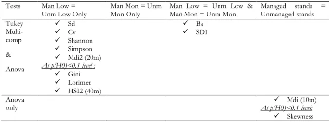
The R script and coding of the model and the analyses of the indices is available in Annex 7. Analyses results consisted of a coefficient for each modality, which were then compared to each other to reject the null hypothesis that managed lowland indices equal unmanaged Lowland indices ( Low=Unm Low) and that managed mountain indices equal unmanaged mountain indices (Man Mon=Unm Mon). To detect differences between the four modalities, a Tukey multiple comparison test was performed with the general linear hypotheses glht function of the simultaneous inference in general parametric models multcomp package (Hothorn et al., 2008). The letter summary of similarities and differences multcompletters function of the visualizations of paired comparisons multcompView package (Graves, 2012) permitted to assign a letter to each modality to flag whether there was a significance difference between modalities.

According to Pinheiro and Bates (2013), the linear mixed-effects model in matrix notation is as follows:

Y

=X

β

+Z

b

+

ε

fixed random error

Where

Xiβ is the fixed effects term,

Zibi is the random effects term, and

Specifically, 𝒀𝒊 = ( 𝒚_𝒊𝟏 𝒚_𝒊𝟐 ⋮ 𝒚_𝒊𝒏𝒊 ) (24)

𝒀

𝑿_𝒊= ( 𝟏 𝒙_𝒊𝟏𝟏 𝒙_𝒊𝟏𝟐 ⋯ 𝒙_𝒊𝟏𝒑 𝟏 𝒙_𝒊𝟐𝟏 𝒙_𝒊𝟐𝟐 ⋯ 𝒙_𝒊𝟐𝒑 ⋮ ⋮ ⋮ ⋯ ⋮ 𝟏 𝒙_𝒊𝒏 𝒊𝟐 𝒙𝒊𝒏𝒊𝟐 ⋯ 𝒙𝒊𝒏𝒊𝒑 ) (25)

𝑿𝒊 is the matrix of the p predictor variables for every single observation in i with a corresponding

p-length fixed effects regression coefficient vector β, 𝒃_𝒊 = ( 𝒃_𝒊𝟎 𝒃_𝒊𝟏 ⋮ 𝒃_𝒊𝒎 ) (26)

𝒃

i

𝒁𝒊 = ( 𝟏 𝒛_𝒊𝟏𝟏 𝒛_𝒊𝟏𝟐 ⋯ 𝒛_𝒊𝟏𝒎 𝟏 𝒙_𝒊𝟐𝟏 𝒛_𝒊𝟐𝟐 ⋯ 𝒛_𝒊𝟐𝒎 ⋮ ⋮ ⋮ ⋯ ⋮ 𝟏 𝒛_𝒊𝒏 𝒊𝟐 𝒛𝒊𝒏𝒊𝟐 ⋯ 𝒛𝒊𝒏𝒊𝒎 ) (27)

𝒁𝒊 is the random effects design matrix for group i and

ɛ_𝒊 = ( ɛ𝒊𝟏 ɛ𝒊𝟐 ⋮ ɛ_𝒊𝒏𝒊 ) (28)

ɛ

i

The assumptions for the linear mixed-effects model are as follows:

 The random-effect vector, b, and the error vector, ε, are independent from each other and have as prior distributions:

b~N(0,σ2D(θ)) (29)

ε~N(0,σ2I) (30)

where D is a positive semi-definite and symmetric matrix, parametrized by a variance component vector θ, I is an n-by-n identity matrix, and σ2 _{is the error variance} (MathWorks, 2015).

In clustered-data situations though as is the case with the GNB data, it is more convenient to organize the model as a series of M clusters and to use the following similar model:

Y

=X

β

+Z

b

+

ε

(Laird & Ware, 1982) Where

- 27 -

Xiβ is the fixed effects term represented by four clusters borne out of the interaction of the parameters “Management” and “Altitude” (Management *Altitude) (i.e. Managed Lowlands, Unmanaged Lowlands, Managed Mountains, Unmanaged Mountains),

Zjbj is the random effects term represented by the 257 forest sites,

εj is the residual variation unaccounted for by the rest of the model,

j=1,…,M, with cluster j including nj observations. The response Yj includes the rows of Y

corresponding to the jth cluster, with Xj and εj defined in the same way. The random effects bj are M realizations of a 𝑞 × 1 vector normally distributed (with mean 0) and a variance matrix Σ 𝑞 × 𝑞, while the matrix Zj is the 𝑛𝑗× 𝑞 design matrix for the jth cluster random effects (Laird & Ware, 1982): Z = ( Z₁ 0 ⋯ 0 0 Z2 ⋯ 0 ⋮ ⋮ ⋱ ⋮ 0 0 0 Z_𝑀 ) (32)

A second simplified analysis test was performed in addition to the Tukey multiple comparison test: an analysis of variance (Anova) with the Anova function of the stats package (R Core Team, 2014). This was meant to test any significant difference between the modality means for management only, not taking into account altitude. The model for this simplified test is:

Y

=X

β

+Z

b

+

ε

Where

Xkβ is the fixed effects term represented by the parameter of “Management”,

Zkbk is the random effects term represented by the 257 forest sites, and

εk is the residual variation unaccounted for by the rest of the model.

Residuals, homoscedasticity and outliers were also reviewed as part of the analyses; however those will not be taken into account at this first stage of analysis. The output of the Tukey multiple comparison tests and the Anova tests for management is available in Annex 8. Statistical significance for all tests was assessed by using the critical probability value (p-value) threshold *p(H0)<0.05.

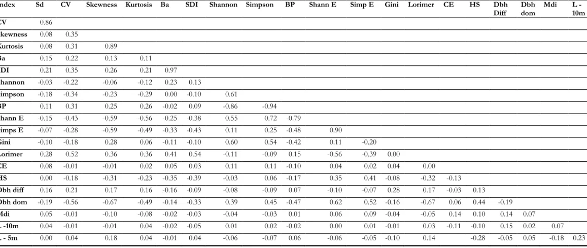
A pairwise correlation analysis was applied to the indices at 10m, 20m and 40m by using the corr.test function of the psych package (Revelle, 2014), which provides the correlation (R2₎ between all the indices (available in Annex 9).

3. RESULTS

The estimators of the four modalities for the 19 indices are shown in Table 4 and are also illustrated as graphs in Annex 10. The values represented in Table 4 are the mean coefficients for each index and the four modalities (Man Low; Unm Low; Man Mon; Unm Mon) at a distance of 40 meters (m), 20 m or 10 m.

The margin of error of the sample means is represented with the notation "±" to indicate the radius (i.e. half the width) of the 95% confidence interval for each mean represented. The margin error was calculated as follows:

Margin of error =Standard error * t distribution critical value

A critical value of 2 (t=2) at a confidence level of 95% was used to calculate the margin of error since the degrees of freedom for each modality were as follows:

Table 3: T distribution critical value

Modality Degrees of freedom value

Managed *Lowland 85 1.99

Unmanaged *Lowland 82 1.99

Managed*Mountain 43 2.02

Unmanaged*Mountain 43 2.02

The results of the Tukey multi-comparison test among the set of modalities are also shown in Table 4 illustrated by a letter display ranging from the letter “a” to the letter “d”. Modalities with means that do not differ significantly at the *p(H0)<0.05 threshold are connected by the same common letter (e.g. “a” is displayed for each modality or “ab” is displayed for a modality not significantly different from a modality with the group label “a” or “b”), while modalities that are significantly different have different letters (e.g. “a”, “b”, “c”, “d”). The different letters only show a significant difference between one or more of the four modalities but the order of the letters is not increasing or descending in terms of the magnitude of the significant difference. This letter display follows the letter-based representation system developed by Piepho (2004) and applied with the multcompletters and multcompView functions in the R software (Graves, 2012) (see Section 2.5 for more details).

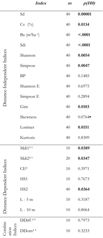
Table 5 illustrates the results of the Anova test meant to test significant differences between the modality means for management only (managed stands vs. unmanaged stands), not taking into account the lowland/mountain altitude dichotomy. The Anova p-values represent the p-values resulting from the Anova test for management, the significance codes are: ***p(H0)< 0.001,

29 -Table 4: Means of indices, margins of error and significant differences4 _{by modality*}

*The indices are: distance-independent indices (standard deviation (Sd), coefficient of variation (Cv),

basal area (Ba), stand density index (SDI), Shannon, Simpson, Berger-Parker (BP), Shannon Evenness (Shannon E), Simpson Evenness (Simpson E), Gini, Skewness, Lorimer, Kurtosis), distance-dependent indices (mean directional index (Mdi), Clark Evans index (CE), Hopkins-Skellam index (HS), L function (L)), combination indices (diameter differentiation index (DDiff), diameter dominance index (DDom)).

4 _{Significant differences are indicated in bold for *p(H0)<0.05 and followed by symbol “▪” for p(H0)<0.1.}

The letters represent any significant difference between one modality and the other modalities. Modalities sharing a letter in the group label are not significantly different.

5 _{Only plots with at least two trees were included for the calculation of the indices.} 6 _{Indices calculated with no edge correction.}

Index m Man Low Unm Low Man Mon Unm Mon

Dis tanc e-Inde pe nde nt I ndic es Sd 40 14.3 ±2.72 a 17.8 ±2.74 b 17.7 ±3.44 ab 19.5 ±3.44 ab Cv (%) 40 46.5 ±5.48 a 53.8 ±5.52 b 53.9 ±7.14 ab 56.7 ±7.14 ab Ba (m2_ha-1_{) 40 20.5 ±2.72 a 24 ±2.72 b 29.4 ±3.44 b 34.1 ±3.44 c} Sdi 40 412 ±50.1 a 480 ±50.2 b 553 ±63.6 b 637 ±63.6 c Shannon 40 1.43 ±0.12 a 1.57 ±0.12 b 1.57 ±0.16 ab 1.67 ±0.16 ab Simpson 40 3.97 ±0.48 a 4.47 ±0.48 b 4.36 ±0.61 ab 4.69 ±0.60 ab BP 40 0.40 ±0.04 a 0.37 ±0.04 a 0.35 ±0.05 a 0.33 ±0.05 a Shannon E 40 0.83 ±0.03 a 0.84 ±0.03 a 0.88 ±0.04 a 0.88±0.04 a Simpson E 40 0.69 ±0.03 a 0.67 ±0.03 a 0.71 ±0.04 a 0.69 ±0.04 a Gini 40 0.25 ±0.03 a▪ 0.28 ±0.03 a▪ 0.28 ±0.03 a 0.30 ±0.03 a Skewness 40 0.39 ±0.22 a 0.53 ±0.22 a 0.31 ±0.28 a 0.52 ±0.28 a Lorimer 40 0.50 ±0.29 a▪ 0.30 ±0.29 a▪ 0.72 ±0.37 a 0.41 ±0.37 a Kurtosis 40 2.97 ±0.44 a 2.95 ±0.44 a 2.71 ±0.60 a 2.90 ±0.60 a Dis tan ce -De pe nd en t I nd ic es Mdi14 5 _{10 2.97 ±0.07 a 2.89 ±0.08 a 2.99 ±0.11 a 2.94 ±0.11 a} Mdi24 5 _{20 3.06 ±0.07 a 2.97 ±0.07 b 2.94 ±0.12 ab 2.93 ±0.12 ab} CE5 _{10 0.19 ±0.01 a 0.18 ±0.01 a 0.19 ±0.02 a 0.19 ±0.02 a} HS1 10 1.64 ±1.10 a 1.75 ±1.04 a 1.52 ±1.78 a 0.95 ±1.78 a HS2 40 0.42 ±0.17 a 0.34 ±0.17 a 0.85 ±0.22 b▪ 0.53 ±0.22 ab▪ L - 5 m 10 0.16 ±0.29 a 0.27 ±0.34 a 0.14 ±0.48 a 0.33 ±0.48 a L - 10 m 10 0.47 ±0.22 a 0.58 ±0.27 a 0.79 ±0.37 a 0.50 ±0.37 a C ombi na tio n In dic es DDiff 4 6 _{10 0.44 ±0.02 a 0.45 ±0.02 a 0.45 ±0.03 a 0.44 ±0.03 a} DDom4 5 _{10 0.36 ±0.07 a 0.35 ±0.05 a 0.48 ±0.12 a 0.44 ±0.12 a}

Table 5: Anova test results for significant differences7 _{between managed and unmanaged stands*}

*The following indices were calculated: distance-independent indices (standard deviation (Sd),

coefficient of variation (Cv), basal area (Ba), stand density index (SDI), Shannon index, Simpson index, Berger-Parker index (BP), Shannon Evenness index (Shannon E), Simpson Evenness index (Simpson E), Gini index, Skewness, Lorimer, Kurtosis), distance-dependent indices (mean directional index (Mdi), Clark Evans index (CE), Hopkins-Skellam index (HS), L function (L)), combination indices (diameter differentiation index (DDiff), diameter dominance index (DDom)).

7 _{Significant differences indicated in bold for *p(H0)<0.05 and followed by symbol “▪” for p(H0)<0.1.} 8 _{Only plots with at least two trees were included for the calculation of the indices.}

9 _{Indices calculated with no edge correction.}

Index m p(H0) Dis tanc e-Inde pe nde nt I ndic es Sd 40 0.00001 Cv (%) 40 0.0134 Ba (m2_ha-1_{) 40 <.0001} Sdi 40 <.0001 Shannon 40 0.0054 Simpson 40 0.0047 BP 40 0.1485 Shannon E 40 0.6975 Simpson E 40 0.2894 Gini 40 0.0103 Skewness 40 0.0764▪ Lorimer 40 0.0151 Kurtosis 40 0.8309 Dis tanc e-De pe nde nt Indic es Mdi14 5 _{10 0.0389} Mdi24 5 _{20 0.0347} CE8 _{10 0.3971} HS1 10 0.7673 HS2 40 0.0364 L - 5 m 10 0.3187 L - 10 m 10 0.8064 C omb in atio n In dic es DDiff 4 9 _{10 0.7973} DDom4 5 _{10 0.3233}