Proceedings of the 14th International Symposium on Computer Music Multidisciplinary Research

HAL Id: hal-02382500

https://hal.archives-ouvertes.fr/hal-02382500

Submitted on 27 Nov 2019

HAL is a multi-disciplinary open access

archive for the deposit and dissemination of

sci-L’archive ouverte pluridisciplinaire HAL, est

destinée au dépôt et à la diffusion de documents

Mitsuko Aramaki, Olivier Derrien, Richard Kronland Martinet, Sølvi Ystad

To cite this version:

Mitsuko Aramaki, Olivier Derrien, Richard Kronland Martinet, Sølvi Ystad. Proceedings of the 14th

International Symposium on Computer Music Multidisciplinary Research. M. Aramaki, O. Derrien, R.

Kronland-Martinet, S. Ystad. Perception, Representations, Image, Sound, Music, Oct 2019, Marseille,

France. 2019, 979-10-97-498-01-6. �hal-02382500�

Proceedings of the

14th International Symposium on

Computer Music Multidisciplinary Research

14 – 18th October, 2019

Marseille, France

Organized by

The Laboratory PRISM

“Perception, Representations, Image, Sound, Music”

Marseille, France

in collaboration with

GMEM “Groupe de Musique Expérimentale de Marseille”

and

The Laboratory PRISM

“Perception, Representations, Image, Sound, Music”

31, chemin Joseph Aiguier

CS 70071

13402 Marseille Cedex 09 - France

October, 2019

All copyrights remain with the authors.

Proceedings Editors: M. Aramaki, O. Derrien,

We are happy to welcome you to the 14th edition of CMMR in Marseille. This is the second CMMR event that takes place in Marseille, but in a slightly different context than in 2013, since the present edition is organized by the new interdis-ciplinary art-science laboratory, PRISM (Perception, Representations, Image, Sound, Music), which very much reflects the spirit of the CMMR conference cycle. PRISM hosts researchers within a large variety of fields, spanning from physics and signal processing, art and aesthetic sciences to medicine and neuro-science that all have a common interest in the perception and representation of image, sound and music. The scientific challenge of PRISM is to reveal how the audible, the visible and their interactions generate new forms of sensitive and/or formal representations of the contemporary world.

CMMR2019 will be the occasion to celebrate the creation of the PRISM and at the same time honor one of its co-founders, researcher, composer and computer music pioneer Jean-Claude Risset who sadly passed away in November 2016, only two months before the laboratory was officially acknowledged. A scientific session followed by an evening concert will be dedicated to him on the first day of the conference.

From the first announcement of the CMMR2019 we received a large response from both scientists and artists who wanted to participate in the conference, ei-ther by organizing special sessions, presenting demos or installations or propos-ing workshops and concerts. Among the 15 scientific sessions that will take place during the conference, eight special sessions that deal with various subjects from sound design, immersive media and mobile devices to music and deafness, em-bodied musical interaction and phenomenology of the conscious experience are scheduled. We are also lucky to have three internationally renowned keynote speakers with us during this edition: John Chowning, Professor Emeritus at Stanford University who will talk about his friend and colleague Jean-Claude Risset, Geoffroy Peeters, Professor at Télécom ParisTech who will talk about past and present research within Music Information Research and Josh McDer-mott, Associate Professor in the Department of Brain and Cognitive Sciences at MIT who will present classic and recent approaches to auditory scene analysis.

contemporary music concert on Wednesday evening. During the last evening, an interactive music concert will take place under the direction of Christophe Héral. Sound installations and a videomusic presentation are also scheduled during the conference.

Finally, in addition to the scientific paper, poster and demo sessions and the artistic program, five satellite workshops are programmed right after the conference on Friday October 18th.

We hope that CMMR2019 will be an unforgettable event for all of you, and wish you a pleasant stay in Marseille.

R. Kronland-Martinet, S. Ystad and M. Aramaki The CMMR2019 symposium chairs

Organization

The 14th International Symposium on Computer Music Multidisciplinary Re-search CMMR2019 “Perception, Representations, Image, Sound, Music” is orga-nized by the laboratory PRISM (CNRS-AMU, UMR 7061, France), GMEM and n+n corsino.

Symposium Chairs

Richard Kronland-Martinet (PRISM, AMU-CNRS, France) Sølvi Ystad (PRISM, AMU-CNRS, France)

Mitsuko Aramaki (PRISM, AMU-CNRS, France) Proceedings Chair

Olivier Derrien (Univ. Toulon, PRISM, France) Paper Chairs

Mitsuko Aramaki (PRISM, AMU-CNRS, France) Ivan Magrin-Chagnolleau (PRISM, AMU-CNRS, France) Programme Chairs

Richard Kronland-Martinet (PRISM, AMU-CNRS, France) Sølvi Ystad (PRISM, AMU-CNRS, France)

Artistic Programme Chairs Norbert Corsino (n+n corsino, France)

Jacques Sapiéga (PRISM, AMU-CNRS, France) Christian Sébille (GMEM, France)

Workshop Chair

Mathieu Barthet (QMUL, United Kingdom) Demo Chair

Poster Chair

Samuel Poirot (PRISM, AMU-CNRS, France) Sponsoring chairs

Antoine Bourachot (PRISM, AMU-CNRS, France) Simon Fargeot (PRISM, AMU-CNRS, France) Samuel Poirot (PRISM, AMU-CNRS, France) Webmaster

Antoine Bourachot (PRISM, AMU-CNRS, France) Local Organising Committee

Mitsuko Aramaki (PRISM CNRS-AMU, France) Mathieu Barthet (QMUL, UK)

Antoine Bourachot (PRISM CNRS-AMU, France) Olivier Derrien (PRISM CNRS-AMU, France) Simon Fargeot (PRISM CNRS-AMU, France) Antoine Gonot (PRISM CNRS-AMU, France)

Richard Kronland-Martinet (PRISM CNRS-AMU, France) Claudine Le Van Phu (PRISM CNRS-AMU, France) Samuel Poirot (PRISM CNRS-AMU, France) Adrien Vidal (PRISM CNRS-AMU, France) Sølvi Ystad (PRISM CNRS-AMU, France) Paper Committee

Mitsuko Aramaki (PRISM CNRS-AMU, France) Mathieu Barthet (QMUL, UK)

Jonathan Bell (PRISM CNRS-AMU, France) Jonathan Berger (Stanford University, USA) Gilberto Bernardes (University of Porto, Portugal) Tifanie Bouchara (CNAM, France)

Sylvain Brétéché (PRISM CNRS-AMU, France) Lionel Bringoux (ISM AMU-CNRS, France)

Marco Buongiorno Nardelli (University of North Texas, USA) Amílcar Cardoso (University of Coimbra, Portugal)

Chris Chafe (Stanford University, USA)

Roger Dannenberg (Carnegie Mellon University, USA) Matthew Davies (INESC TEC, Portugal)

Olivier Derrien (PRISM CNRS-AMU, France) Christine Esclapez (PRISM CNRS-AMU, France) Georg Essl (University of Wisconsin, USA) Clément François (LPL CNRS-AMU, France) Rolf Inge Godøy (University of Oslo, Norway) Antoine Gonot (PRISM CNRS-AMU, France) Keiji Hirata (Future University Hakodate, Japan)

Kristoffer Jensen (re-new - Forum for Digital Art, Denmark) Richard Kronland-Martinet (PRISM CNRS-AMU, France) Marc Leman (University of Gent, Belgium)

James Leonard (Université Grenoble Alpes, France) Luca Ludovico (University of Milan, Italy)

Olivier Macherey (LMA CNRS-AMU, France)

Ivan Magrin-Chagnolleau (PRISM CNRS-AMU, France) Sylvain Marchand (University of La Rochelle, France) David Moffat (QMUL, UK)

Johan Pauwels (QMUL, UK)

Samuel Poirot (PRISM CNRS-AMU, France) Matthew Roger (Queen’s University Belfast, UK)

Charalampos Saitis (Technical University of Berlin, Germany) Emery Schubert (University of New South Wales, Sydney, Australia) Diemo Schwarz (IRCAM, France)

Rod Selfridge (QMUL, UK)

Stefania Serafin (Aalborg University Copenhagen, Denmark) Peter Sinclair (PRISM CNRS-AMU, France)

Julius Smith (Stanford University, USA) Bob L. Sturm (Aalborg University, Denmark) Patrick Susini (IRCAM, France)

Atau Tanaka (Goldsmiths, University of London, UK) Vincent Tiffon (PRISM CNRS-AMU, France)

Bruno Torrésani (I2M CNRS-AMU, France)

Jérôme Villeneuve (Université Grenoble Alpes, France) Jean Vion-Dury (PRISM CNRS-AMU, France) Grégory Wallet (Université de Rennes 2, France) Marcelo Wanderley (McGill University, Canada) Duncan Williams (University of York, UK) Sølvi Ystad (PRISM CNRS-AMU, France)

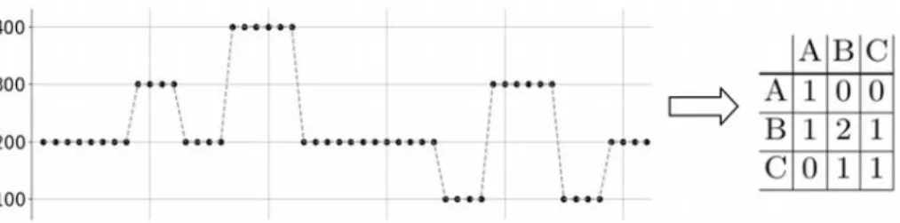
Table of Contents

Oral Session - Computational Musicology 1

Modal Logic for Tonal Music . . . 13 Satoshi Tojo

John Cage’s Number Pieces, a Geometric Interpretation of “Time

Brackets” Notation . . . 25 Benny Sluchin and Mikhail Malt

Modelling 4-dimensional Tonal Pitch Spaces with Hopf Fibration . . . 38

Hanlin Hu and David Gerhard

Oral Session - Computational Musicology 2

Automatic Dastgah Recognition using Markov Models . . . 51

Luciano Ciamarone, Baris Bozkurt, and Xavier Serra

Chord Function Identification with Modulation Detection Based on HMM 59 Yui Uehara, Eita Nakamura, and Satoshi Tojo

Oral Session - Music Production and Composition

Tools

(Re)purposing Creative Commons Audio for Soundscape Composition

using Playsound . . . 71 Alessia Milo, Ariane Stolfi, and Mathieu Barthet

Generating Walking Bass Lines with HMM . . . 83 Ayumi Shiga and Tetsuro Kitahara

Programming in Style with Bach . . . 91 Andrea Agostini, Daniele Ghisi, and Jean-Louis Giavitto

Method and System for Aligning Audio Description to a Live Musical

Theater Performance . . . 103 Dirk Vander Wilt and Morwaread Mary Farbood

Special Session - Jean-Claude Risset and Beyond

Jean-Claude Risset and his Interdisciplinary Practice: What do the

Archives Tell Us? . . . 112 Vincent Tiffon

Spatial Perception of Risset Notches . . . 118 Julián Villegas

Machine Learning for Computer Music Multidisciplinary Research: A

Practical Case Study . . . 127 Hugo Scurto and Axel Chemla-Romeu-Santos

Connecting Circle Maps, Waveshaping, and Phase Modulation via

Iterative Phase Functions and Projections . . . 139 Georg Essl

Mathematics and Music: Loves and Fights . . . 151 Thierry Paul

Special Session - The Process of Sound Design

(Tools, Methods, Productions)

Exploring Design Cognition in Voice-Driven Sound Sketching and

Synthesis . . . 157 Stefano Delle Monache and Davide Rocchesso

Morphing Musical Instrument Sounds with the Sound Morphing Toolbox 171 Marcelo Caetano

Mapping Sound Properties and Oenological Characters by a Collaborative Sound Design Approach - Towards an Augmented

Experience . . . 183 Nicolas Misdariis, Patrick Susini, Olivier Houix, Roque Rivas,

Clément Cerles, Eric Lebel, Alice Tetienne, and Aliette Duquesne

Kinetic Design - From Sound Spatialisation to Kinetic Music . . . 195 Roland Cahen

Special Session - Sonic Interaction for Immersive

Media - Virtual and Augmented Reality

Augmented Live Music Performance using Mixed Reality and Emotion

Feedback . . . 210 Rod Selfridge and Mathieu Barthet

Designing Virtual Soundscapes for Alzheimer’s Disease Care . . . 222 Frédéric Voisin

ARLooper: a Mobile AR Application for Collaborative Sound Recording

and Performance . . . 233 Sihwa Park

Singing in Virtual Reality with the Danish National Children’s Choir . . . . 241 Stefania Serafin, Ali Adjorlu, Lars Andersen, and Nicklas Andersen

gravityZERO, an Installation Work for Virtual Environment. . . 254 Suguru Goto, Satoru Higa, John Smith, and Chihiro Suzuki

Special Session - Music and Deafness: From the Ear

to the Body

Why People with a Cochlear Implant Listen to Music . . . 264 Jérémy Marozeau

The ‘Deaf listening’. Bodily Qualities and Modalities of Musical

Perception for the Deaf . . . 276 Sylvain Brétéché

Objective Evaluation of Ideal Time-Frequency Masking for Music

Complexity Reduction in Cochlear Implants . . . 286 Anil Nagathil and Rainer Martin

Evaluation of New Music Compositions in Live Concerts by Cochlear

Implant Users and Normal Hearing Listeners . . . 294 Waldo Nogueira

Special Session - Embodied Musical Interaction

Embodied Cognition in Performers of Large Acoustic Instruments as a

Method of Designing New Large Digital Musical Instruments . . . 306 Lia Mice and Andrew P. McPherson

An Ecosystemic Approach to Augmenting Sonic Meditation Practices . . . 318 Rory Hoy and Doug Van Nort

Gesture-Timbre Space: Multidimensional Feature Mapping Using

Machine Learning & Concatenative Synthesis . . . 326 Michael Zbyszyński, Balandino Di Donato, and Atau Tanaka

Special Session - Phenomenology of Conscious

Experience

Beyond the Semantic Differential: Timbre Semantics as Crossmodal

Correspondences . . . 338 Charalampos Saitis

Generative Grammar Based on Arithmetic Operations for Realtime

Composition . . . 346 Guido Kramann

A Phenomenological Approach to Investigate the Pre-reflexive Contents

of Consciousness during Sound Production . . . 361 Marie Degrandi, Gaëlle Mougin, Thomas Bordonné, Mitsuko

Aramaki, Sølvi Ystad, Richard Kronland-Martinet, and Jean Vion-Dury

Special Session - Notation and Instruments

Distributed on Mobile devices

Mobile Music with the Faust Programming Language . . . 371 Romain Michon, Yann Orlarey, Stéphane Letz, Dominique Fober,

Catinca Dumitrascu, and Laurent Grisoni

COMPOSITES 1: An Exploration into Real-Time Animated Notation

in the Web Browser . . . 383 Daniel McKemie

Realtime Collaborative Annotation of Music Scores with Dezrann . . . 393 Ling Ma, Mathieu Giraud, and Emmanuel Leguy

Distributed Scores and Audio on Mobile Devices in the Music for a

Multidisciplinary Performance . . . 401 Pedro Louzeiro

The BabelBox: an Embedded System for Score Distribution on

Raspberry Pi with INScore, SmartVox and BabelScores . . . 413 Jonathan Bell, Dominique Fober, Daniel Fígols-Cuevas, and Pedro

Garcia-Velasquez

Oral Session - Music Information Retrieval - Music,

Emotion and Representation 1

Methods and Datasets for DJ-Mix Reverse Engineering . . . 426 Diemo Schwarz and Dominique Fourer

Identifying Listener-informed Features for Modeling Time-varying

Emotion Perception . . . 438 Simin Yang, Elaine Chew, and Mathieu Barthet

Towards Deep Learning Strategies for Transcribing Electroacoustic Music 450 Matthias Nowakowski, Christof Weiß, and Jakob Abeßer

Special Session - Improvisation, Expectations and

Collaborations

Improvisation and Environment . . . 462 Christophe Charles

Improvisation: Thinking and Acting the World . . . 470 Carmen Pardo Salgado

Developing a Method for Identifying Improvisation Strategies in Jazz Duos 482 Torbjörn Gulz, Andre Holzapfel, and Anders Friberg

Instruments and Sounds as Objects of Improvisation in Collective

Computer Music Practice . . . 490 Jérôme Villeneuve, James Leonard, and Olivier Tache

Oral Session - Audio Signal Processing - Music

Structure Analysis

Melody Slot Machine: Controlling the Performance of a Holographic

Performer . . . 502 Masatoshi Hamanaka

MUSICNTWRK: Data Tools for Music Theory, Analysis and Composition . . 514 Marco Buongiorno Nardelli

Feasibility Study of Deep Frequency Modulation Synthesis . . . 526 Keiji Hirata, Masatoshi Hamanaka, and Satoshi Tojo

Description of Monophonic Attacks in Reverberant Environments via

Spectral Modeling . . . 534 Thiago A. M. Campolina and Mauricio Alves Loureiro

Oral Session Auditory perception and cognition

-Music and the Brain 1

Modeling Human Experts’ Identification of Orchestral Blends Using

Symbolic Information . . . 544 Aurélien Antoine, Philippe Depalle, Philippe Macnab-Séguin, and

Stephen McAdams

The Effect of Auditory Pulse Clarity on Sensorimotor Synchronization . . . 556 Prithvi Kantan, Rareş Ştefan Alecu, and Sofia Dahl

The MUST Set and Toolbox . . . 564 Ana Clemente, Manel Vila-Vidal, Marcus T. Pearce, and Marcos

Nadal

Oral Session - Music Information Retrieval - Music,

Emotion and Representation 2

Ensemble Size Classification in Colombian Andean String Music

Recordings . . . 565 Sascha Grollmisch, Estefanía Cano, Fernando Mora Ángel, and

Gustavo López Gil

Towards User-informed Beat Tracking of Musical Audio . . . 577 António Sá Pinto and Matthew E. P. Davies

Drum Fills Detection and Generation . . . 589 Frédéric Tamagnan and Yi-Hsuan Yang

Discriminative Feature Enhancement by Supervised Learning for Cover

Song Identification . . . 598 Yu Zhesong, Chen Xiaoou, and Yang Deshun

Oral Session Auditory Perception and Cognition

-Music and the Brain 2

Perception of the Object Attributes for Sound Synthesis Purposes . . . 607 Antoine Bourachot, Khoubeib Kanzari, Mitsuko Aramaki, Sølvi

Ystad, and Richard Kronland-Martinet

A Proposal of Emotion Evocative Sound Compositions for Therapeutic

Purposes . . . 617 Gabriela Salim Spagnol, Li Hui Ling, Li Min Li, and Jônatas

Manzolli

On the Influence of Non-Linear Phenomena on Perceived Interactions

in Percussive Instruments . . . 629 Samuel Poirot, Stefan Bilbao, Sølvi Ystad, Mitsuko Aramaki, and

Richard Kronland-Martinet

Oral Session - Ubiquitous Music

Musicality Centred Interaction Design to Ubimus: a First Discussion . . . . 640 Leandro Costalonga, Evandro Miletto, and Marcelo S. Pimenta

A Soundtrack for Atravessamentos: Expanding Ecologically Grounded

Methods for Ubiquitous Music Collaborations . . . 652 Luzilei Aliel, Damián Keller, and Valeska Alvim

The Analogue Computer as a Voltage-Controlled Synthesiser . . . 663 Victor Lazzarini and Joseph Timoney

Sounding Spaces for Ubiquitous Music Creation . . . 675 Marcella Mandanici

Ubiquitous Music, Gelassenheit and the Metaphysics of Presence:

Hijacking the Live Score Piece Ntrallazzu 4 . . . 685 Marcello Messina and Luzilei Aliel

Live Patching and Remote Interaction: A Practice-Based,

Intercontinental Approach to Kiwi . . . 696 Marcello Messina, João Svidzinski, Deivid de Menezes Bezerra, and

David Ferreira da Costa

Poster Session

Flexible Interfaces: Future Developments for Post-WIMP Interfaces . . . 704 Benjamin Bressolette and Michel Beaudouin-Lafon

Geysir: Musical Translation of Geological Noise . . . 712 Christopher Luna-Mega and Jon Gomez

Visual Representation of Musical Rhythm in Relation to Music

Technology Interfaces - an Overview . . . 725 Mattias Sköld

A Tree Based Language for Music Score Description . . . 737 Dominique Fober, Yann Orlarey, Stéphane Letz, and Romain

Michon

Surveying Digital Musical Instrument Use Across Diverse Communities

of Practice . . . 745 John Sullivan and Marcelo M. Wanderley

Systematising the Field of Electronic Sound Generation . . . 757 Florian Zwißler and Michael Oehler

Movement Patterns in the Harmonic Walk Interactive Environment . . . 765 Marcella Mandanici, Cumhur Erkut, Razvan Paisa, and Stefania

Serafin

Embodiment and Interaction as Common Ground for Emotional

Experience in Music . . . 777 Hiroko Terasawa, Reiko Hoshi-Shiba, and Kiyoshi Furukawa

Computer Generation and Perception Evaluation of Music-Emotion

Associations . . . 789 Mariana Seiça, Ana Rodrigues, Amílcar Cardoso, Pedro Martins,

and Penousal Machado

Situating Research in Sound Art and Design: The Contextualization of

Ecosound . . . 801 Frank Pecquet

The Statistical Properties of Tonal and Atonal Music Pieces . . . 815 Karolina Martinson and Piotr Zieliński

Webmapper: A Tool for Visualizing and Manipulating Mappings in

Digital Musical Instruments . . . 823 Johnty Wang, Joseph Malloch, Stephen Sinclair, Jonathan

Wilansky, Aaron Krajeski, and Marcelo M. Wanderley

The Tragedy Paradox in Music: Empathy and Catharsis as an Answer? . . 835 Catarina Viegas, António M. Duarte, and Helder Coelho

‘Visual-Music’? The Deaf Experience. ‘Vusicality’ and Sign-singing . . . 846 Sylvain Brétéché

Machines that Listen: Towards a Machine Listening Model based on

Perceptual Descriptors . . . 858 Marco Buongiorno Nardelli, Mitsuko Aramaki, Sølvi Ystad, and

Richard Kronland-Martinet

Pedaling Technique Enhancement: a Comparison between Auditive and

Visual Feedbacks. . . 869 Adrien Vidal, Denis Bertin, Richard Kronland-Martinet, and

Christophe Bourdin

Musical Gestures: An Empirical Study Exploring Associations between Dynamically Changing Sound Parameters of Granular Synthesis with

Hand Movements . . . 880 Eirini-Chrysovalantou Meimaridou, George Athanasopoulos, and

Emilios Cambouropoulos

Concatenative Synthesis Applied to Rhythm. . . 892 Francisco Monteiro, Amílcar Cardoso, Pedro Martins, and Fernando

Perdigão

Enhancing Vocal Melody Transcription with Auxiliary Accompaniment

Information . . . 904 Junyan Jiang, Wei Li, and Gus G. Xia

Extraction of Rhythmical Features with the Gabor Scattering Transform . 916 Daniel Haider and Peter Balazs

Kuroscillator: A Max-MSP Object for Sound Synthesis using

Coupled-Oscillator Networks . . . 924 Nolan Lem and Yann Orlarey

Distinguishing Chinese Guqin and Western Baroque Pieces based on

Statistical Model Analysis of Melodies . . . 931 Yusong Wu and Shengchen Li

End-to-end Classification of Ballroom Dancing Music Using Machine

Learning . . . 943 Noémie Voss and Phong Nguyen

An Evidence of the Role of the Cellists’ Postural Movements in the

Score Metric Cohesion . . . 954 Jocelyn Rozé, Mitsuko Aramaki, Richard Kronland-Martinet, and

Sølvi Ystad

Zero-Emission Vehicles Sonification Strategy Based on Shepard-Risset

Glissando . . . 966 Sébastien Denjean, Richard Kronland-Martinet, Vincent Roussarie,

and Sølvi Ystad

Demo Papers

“Tales From the Humanitat” - A Multiplayer Online Co-Creation

Environment . . . 977 Geoffrey Edwards, Jocelyne Kiss, and Juan Nino

Auditory Gestalt Formation for Exploring Dynamic Triggering

Earthquakes . . . 983 Masaki Matsubara, Yota Morimoto, and Takahiko Uchide

Minimal Reduction . . . 988 Christopher Chraca

M O D U L O . . . 993 Guido Kramann

A Real-time Synthesizer of Naturalistic Congruent Audio-Haptic Textures 1000 Khoubeib Kanzari, Corentin Bernard, Jocelyn Monnoyer, Sébastien

Denjean, Michaël Wiertlewski, and Sølvi Ystad

CompoVOX 2: Generating Melodies and Soundprint from Voice in Real

Time . . . 1005 Daniel Molina Villota, Antonio Jurado-Navas, Isabel Barbancho

Coretet: a 21st Century Virtual Interface for Musical Expression . . . 1010 Rob Hamilton

Modal Logic for Tonal Music

Satoshi Tojo?

Japan Advanced Institute of Science and Technology tojo@jaist.ac.jp

Abstract. It is generally accepted that the origin of music and language is one and the same. Thus far, many syntactic theories of music have been proposed, however, all these e↵orts mainly concern generative syntax. Al-though such syntax is advantageous in constructing hierarchical tree, it is weak in representing mutual references in the tree. In this research, we propose the annotation of tree with modal logic, by which the reference from each pitch event to regions with harmonic functions are clarified. In addition, while the generative syntax constructs the tree in the top-down way, the modal interpretation gives the incremental construction accord-ing to the progression of music. Therefore, we can naturally interpret our theory as the expectation–realization model that is more familiar to our human recognition of music.

Keywords: Generative Syntax, Modal Logic, Kripke semantics

1

Introduction

What is the semantics of music? In general, the semantics is distinguished be-tween the reference to the internal structure and that to the outer worlds. Even

though we could somewhat guess what the external references mean,1 _still

re-mains the question what is the internal semantics. Meyer [13] argued that we could define an innate meaning independent of the external references. Although there should be a big discussion more for this, we contend that we could devise a formal method to clarify the internal references.

Assuming that the origin of music and language is one and the same [18], we consider incorporating Montagovian semantics [6], as a parallelism between

syntactic structure and logical forms, into music.2

In this work, we propose to employ the modal logic to represent internal references in music. Such modal operators as

?_{This work is supported by JSPS kaken 16H01744.}

1 _{Koelsch [12] further distinguished the three levels of the reference to the outer worlds;}

(i) the simple imitation of sounds by instruments, (ii) the implication of human emotions, and (iii) the artificial connection to our social behavior.

2 _{We need to take care of the ambiguity of what semantics means. In Montagovian}

theory, the syntax of natural language is those written by categorial grammar and the semantics is written by logical formuale, while in mathematical logic the formal language (logic) has its own syntax and its semantics is given by set theory or by algebra.

⇤ · · · For all the time points in some neighborhood region ⌃ · · · A time point exists in any neighborhood region

denote the accessibility from each pitch event in music to specified regions, and thus, we can clarify the inter-region relationship in a piece.

Thus far, many linguistic approaches have been made to analyze the music structure, however, almost all these e↵orts concern the generative syntax, based on Context-free Grammar (CFG) by Chomsky [1, 2]. However, the non-terminal symbols in the production rules, which appear as nodes in the tree, are often vague in music; in some cases they may represent the saliency among pitch events and in other cases overlaying relations of functional regions. Also, the hierarchical construction of tree is weak in representing mutual phrasal relationship. In this work, we reinterpret those generative grammar rules in the X-bar theory [3], and show their heads explicitly. Then, we define the annotations of rules in logical formulae, and give a rigorous semantics by modal logic.

This reinterpretation accompanies one more significant aspect. The tree struc-ture is constructed by production rules in the top-down way. However, when we listen to or compose music, we recognize it in the chronological order according to the progression of time. With our method, those rules would be transformed to construct a tree in the incremental way.

This paper is organized as follows. In the following section, we survey the syntactic studies in music. Next, we introduce the modal logic as formal lan-guage to represent the internal structure of music, regarding its neighborhood semantics as the inclusion and the order of time intervals, and then, we give a concrete example of analysis by modal logic. In the final section, we summarize our contribution and discuss our future tasks.

2

Syntactic Theory of Music

Thus far, many linguists and musicologists have achieved to implement the mu-sic parser, beginning from Winograd [19]. Some works were based on specific grammar theories; Tojo [17] employed Head-driven Phrase Structure Grammar (HPSG) and Steedman et al. [8] Combinatory Categorial Grammar (CCG). In recent years, furthermore, two distinguished works are shown; one is exGTTM by Hamanaka et al. [11] based on Generative Theory of Tonal Music (GTTM) [10] and the other is Generative Syntax Model (GSM) by Rohmeier [16].

2.1 Brief Introduction of GSM

We briefly introduce GSM with its abridged grammar for convenience. First we introduce the basic sets

R = { TR, SR, DR } (region)

F = { t, s, d, tp, sp, dp, tcp } (function)

The P (piece) is the start symbol of production rules. It introduces TR (tonic region)

P _{! TR,}

In the next level, TR generates DR (dominant region) and SR (subdominant region), and in the further downward level they result in t (tonic), d (dominant), s (subdominant).

TR_{! DR t} TR_{! t}

DR_{! SR d} DR_{! d}

TR! TR DR SR! s

Also, each of t, d, s may result in tp (tonic parallel), tcp (tonic counter-parallel), dp (dominant parallel), sp (subdominant parallel) of Hugo Riemann [9].

t! tp | tcp, s ! sp, d ! dp

where the vertical bar (‘_{|’) shows the ‘or’ alternatives. In addition, there are}

scale-dgree rules, which maps function names to degrees, e.g.,

t_{! I, tp ! VI | III, s ! IV, d ! V | VII, and so on.}

Furthermore, [16] employed the rules of secondary dominant, and that of mod-ulation.

However, the formalism of GSM is partially inconvenient since the interpre-tation of

XR_{! XR XR (XR 2 R)}

is ambiguous as to which is the head. Rather, we prefer to rigorously define heads, distinguishing region rules from harmonic function rules.

2.2 X-barred GSM

Here, we introduce the notion of head, employing the X-bar theory [3].3_{A binary}

production in Chomsky Normal Form (CNF) should be rewritten with the parent

category X0 _{and the head daughter category X, as follows.}

(

X0 ! Spec X

X0 _{! X Comp}

where Spec stands for specifier and Comp for complement.4 _{When X in the}

right-hand side already includes a prime (0), X0 in the left-hand side becomes

doubly primed (00) recursively.

3 _{The latest Chomskian school has abandoned X-bar theory, and instead they explain}

every syntactic phenomena only by merge and recursion [4].

4 _{Note that notion of head resides also in Combinatory Categorial Grammar (CCG),}

Since we do not use those degree rules, our simplified GSM rules becomes as

follows, where_{F = {tnc, dom, sub}.}

TR0 ! DR TR T R! tnc

DR0_{! SR DR} DR_{! dom}

TR00! TR0 TR SR! sub

TR00_{! TR TR}0

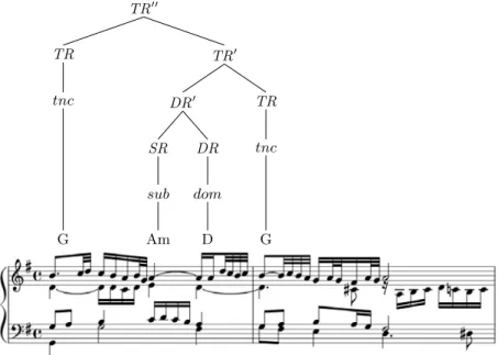
We show an example of syntactic tree by our rules in Fig. 1.

TR00 TR tnc G TR0 DR0 SR sub Am DR dom D TR tnc G

Fig. 1. J. S. Bach: “Liebster Jesu, Wir Sind Hier ”, BWV731

3

Semantics in Logic

3.1 Modal Logic

A modal logic consists of such syntax as follows.

:= p| ¬ | _ | ⇤

where⇤ represents, intuitively, ‘necessarily .’ In order to give a formal

seman-tics to modal logic, we provide a Kripke frame which is a tripletM = hW, R, V i.

when w0 _{is accessible from w we write wRw}0_{. V is a valuation for each atomic}

proposition. Employing the negation connective, we also introduce5

^ ⌘ ¬(¬ _ ¬ ), ⌘ ¬ _ , and ⌃ ⌘ ¬⇤¬ .

Now, we give the semantics of ‘⇤’ operator, and its dual operator ‘⌃’, as

follows.

M, w |= ⇤ i↵ for all w0(wRw0)_{2 W, M, w}0_|=

M, w |= ⌃ i↵ there exists w0(wRw0)_{2 W and M, w}0_|=

that is,⇤ holds in w if and only if holds in all the accessible worlds w0 _from

w, and ⌃ holds in w if and only if there exists an accessible world w0 _where

holds.

We also read ‘⇤ ’ as ‘(a certain agent) knows ’ in epistemic logic since the

knowledge of agent is a part of propositions which are true to her after

consid-ering (accessing) every possibility. In deontic logic ‘⇤ ’ means ‘ is obligatory.’

In our study, this formula means persists for a certain extent of time.

Topological Semantics In Kripke semantics, we have presupposed that a set of possible worlds is a finite number of discrete ones, however, we can naturally

extend the notion to a continuous space. Given a mother set X, letP(X) be the

powerset of X and letT ⇢ P(X). We call T is a topology if it satisfies

1. for_O1,O22 T , O1\ O22 T .

2. for any (possibly infinite) index set ⇤, if each Oi(i2 ⇤) 2 T , [i2⇤Oi2 T .

3. X,; 2 T .

A topological semantics of modal logic adopts a topology _{T instead of}

ac-cessibility relation R, rereading possible worlds as geometric points in a more

general way. A member of_{T is an open set that does not have intuitively hard}

boundaries in a metric space, or an open ball.

M, w |= ⇤ i↵ there exists O 2 T (w 2 O), for all w02 O, M, w0|= (1)

M, w |= ⌃ i↵ for all O 2 T (w 2 O), there exists w0 2 O, M, w0 |= (2)

that is, ⇤ holds if and only if there is a set in T in which at all the points

holds, while⌃ holds if and only if in any set in T there is a point at which

holds.

Among various arbitrary topologies, the discrete topology consists of all the

subset of mother set X, that is, _{T = P(X). Then, every point is distinguished}

from each other.

When w_{|= , in any O including w, w |= , so that Axiom}

⌃ (T⇤)

inevitably holds.6

5 _{Note that ‘ ’ is not a set inclusion but a logical implication.} 6 _{Axiom T is⇤ and T}⇤_{is its dual form.}

Neighborhood Semantics We call N (w) is a set of neighborhoods of w. When we are given neighborhoods as a set of open balls for each point, we can construct

a topology by a technique called filtration.7 _{The semantics of modal operators}

are defined as follows.

M, w |= ⇤ i↵ J K 2 N(w)

M, w |= ⌃ i↵ J Kc

62 N(w)

whereJ K = {w | M, w |= }, and J Kc_{= W}

\ J K is the complement set of W .

3.2 Temporal Logic

Now we translate modal logic to temporal logic.

– Let a point (a world in Kripke semantics) be a time point. – Let an open ball be an open time interval.

Here, we provide two di↵erent relations among intervals.

⌧1 ⌧2: ⌧1temporally precedes ⌧2

⌧1✓ ⌧2: ⌧1is temporally included in ⌧2

However, this formalism is confusing since our intuitive interpretation of the precedence relation is for time points while the inclusion relation refers to in-tervals. In order to treat points and intervals impartially, we employ topological semantics, as follows.

Let ‘ ’ be the total order of ⌧i’s. Then, the convex open ball is such that for

⌧, ⌧0 _{2 O any ⌧}00 _{(⌧ ⌧}00 _{⌧ )2 O. Then, let T be}

T = {O 2 T | O is convex}.

From now on, we regard a convex open ball is a time interval. In short, we write

(⌧i, ⌧j) to represent the minimum convex open ball including ⌧i and ⌧j; if an

open ball consists of a single pitch event ⌧i we write (⌧i). Meanwhile, {⌧i, ⌧j}

represents a set consists of two time points and we write {⌧1, ⌧2,· · · } |= for

⌧i|= (i = 1, 2,· · · ).

4

Logical Annotation in Music

Our task in this paper is to annotate the syntactic tree by such formulae and to identify the harmonic regions among the time intervals. To be precise, according to a pitch event found at each time point ⌧ , we aim at fixing the neighborhood N (⌧ ) to validate the formula at ⌧ , and name those intervals as regions.

7 _{N (w) is a filter when N (w) is a set of neighborhoods of w, and for any U}

2 N(w) there exists V (⇢ U) 2 N(w) and for all w0_{2 V, U 2 N(w}0_).

4.1 Logical Formula for Syntactic Rule Now we give the syntax of logical formulae as follows.

::= f (x)| f(c) | ¬ | _ | 8x | ⇤

where f 2 F, c 2 O supplemented with chord name variables. We provide other

logical connectives^ and as before, as well as modal operator⌃ and 9x ⌘

¬8x¬ . We often write ⌧ |= when holds at time ⌧ omitting the frame _M

for simplicity; notice that is not a pitch event itself but a proposition with

function name as predicate.

In order to implement a progression model instead of a generation model, we employ Earley’s algorithm [7]. Let us consider a generative (production) rule

A_{! B C. Then the rule is evoked and executed in the following process.}

1. Observe an pitch event with a harmonic function.

2. Find such generative rule(s) that the first item of the right-hand side B matches the observation.

3. To complete the upper category A residing at the left-hand side of ‘!’,

expect the second item in the right-hand side C of the rule.

We provide logical formulae with variables, corresponding to each syntactic rule, including

⌃f(x) · · · There is a pitch event x with function f in the neighborhood. ⇤⌃f(x) · · · Anywhere in some region (‘⇤’), we can access (‘⌃’) f(x).

Tentatively instead of _{F = {tnc, dom, sub}, let head, spc, cmp 2 F, standing}

for X, Spec, and Comp, respectively, in X-bar rules. The syntactic head must exist while specifiers and complements may arbitrarily be accompanied. Then, to annotate each X-bar rule with logical formula, we propose the following

quan-tifications. ₈ > < > : 9x[head(x) ^ · · · ] 8x[spc(x) · · · ] 8x[cmp(x) · · · ]

Here, we combine the above components, considering spc and cmp appear before and after the head, respectively, in accordance with the usual dual relation

of_8x[ ] versus_{9x[ ^ ],}8 _{as follows.}

– For X0_{! Spec X with X ! head and Spec ! spc,}

8x[spc(x) 9y[⌃head(y) ^ ⇤⌃head(y)]]. (3)

– For X0_{! X Comp with X ! head and Comp ! cmp,}

9x[head(x) ^ 8y[⌃cmp(y) ⇤⌃head(x)]]. (4)

8 _{If we negate the whole}

8x[ ] as _¬8x[ ] we obtain _{9x[ ^ ¬ ], and vice} versa.

The intuitive reading is that if we observe spc(x) there exists a head event

head (y) in the neighborhood as ⌃head(y). The combined events could form a

region (a temporal extent), that is a neighborhood_{O and ⌧(2 O) |= ⌃head(y),}

that is ⌧ _{|= ⇤⌃head(y). If we observe head(x) first it is possibly accompanied}

by cmp(y) in the neighborhood, that is⌃cmp(y). Then, there should be a wider

region in which⇤⌃head(x) holds.

Example 1 For DR0_{! SR DR, since d is the head, we expect that the}

following formula according to (3) would be satisfied.

8x[sub(x) 9y[⌃dom(y) ^ ⇤⌃dom(y)]].

Let C be a subdominant in Gmaj found at ⌧2 as ⌧2 |= sub(C). Though

⌧2|= ⌃dom(y) y is not bound yet. Next, we envisage we find dominant

in the neighborhood of ⌧2. Let ⌧3|= dom(D). This meets the expectation

at ⌧2as ⌧2|= ⌃dom(D). Also by T⇤, ⌧3|= ⌃dom(D) and thus {⌧2, ⌧3} |=

⇤⌃dom(D). To be reminiscent of original region names, (⌧2) is SR and

(⌧2, ⌧3) is DR, respectively. ⌅

Example 2 For TR00! TR0 TR, we expect

9x[tnc(x) ^ 8y[⌃tnc(y) ⇤⌃tnc(x)]]

would be satisfied according to (4). Let ⌧7 |= tnc(G). If ⌧9 |= tnc(Em)

we can consider Em is a complement of head G, and {⌧7, ⌧8, ⌧9} |=

⇤⌃tnc(G). Then, (⌧7, ⌧9) becomes TR. ⌅

We summarize our logical formulae corresponding to abridged X-bar syntac-tic rules in Table 1.

TR0_{! DR TR 8x[dom(x) 9y[⌃tnc(y) ^ ⇤⌃tnc(y)]]} DR0_{! SR DR 8x[sub(x) 9y[⌃dom(y) ^ ⇤⌃dom(y)]]} TR00_{! TR}0 TR _{9x[tnc(x) ^ 8y[⌃tnc(y)} ⇤⌃tnc(x)]] TR00_{! TR TR}0 _{8x[tnc(x) 9y[⌃tnc(y) ^ ⇤⌃tnc(y)]]} TR! tnc 9x[tnc(x) ^ ⇤⌃tnc(x)]

DR! dom 9x[dom(x) ^ ⇤⌃dom(x)] SR! sub 9x[sub(x) ^ ⇤⌃sub(x)]

4.2 Valuation with Key

In general, a logical formula in modal logic is evaluated, that is to decide true

or false, given a Kripke frame or simply model _{M with possible world w as}

follows.

M, w |= .

In our case, a possible world is a time point ⌧ and the frameM is either topology

T or the neighborhoods, thus

M, ⌧ |= .

Especially, when includes modal operators, our task has been to fix N (⌧ ) so

as to validate .

Besides, we need key information in our context of music on the left-hand

side of ‘_{|=’. When we observe a set of notes {D, E], A} at a certain time point}

in a music piece, we recognize the pitch event as chord D, though we may not

yet be aware of the scale degree and its key. A chord inO possesses a function

inF dependent on a key. If the context is G major, we can assign the dominant

function to this D. That is, tnc(G), dom(D), sub(C) all hold in G major while not in C major.

Since we have provided a topology or a neighborhood, we need to detail the

left-hand side of ‘_{|=’, as}

Gmaj,M, ⌧ |= dom(D).

Or, in general, K._{M, ⌧ |=} where K _{2 K. For simplicity, in the remaining}

discussion we omit such key information as long as there is no confusion.

4.3 Detailed Analysis

As an example, we detail the analysis for the beginning part of “Liebster Jesu, Wir Sind Hier ” of Fig. 1, in Table 2.

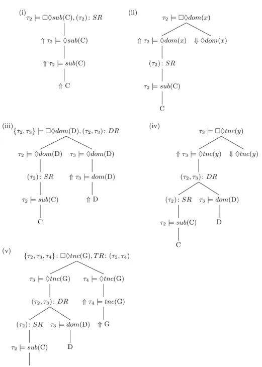
Fig. 2 shows the bottom half of the processes in Table 2, (i) the recognition of subdominant C evokes the expectation of dominant, (ii) the expectation to detect a dominant, (iii) The detection of dominant D satisfies the DR and evokes another expectation of tonic, (iv) the expectation towards the tonic, and (v) The final G satisfies the tonic function and the completion of the tree. In Fig. 3, we show the suggested regions by our analysis.

5

Discussion

In this paper, we have proposed the logical semantics of music. We employed the X-bar theory and reinterpreted the existing grammar rules according to the notation. Thereafter, we have shown the principles of producing logical formulae. Finally, we have shown the analysis example based on Generative Syntax Model. Our contributions are two-fold. First, we have given a clear accessibility re-lations, from each pitch event to regions in the tree structure, in terms of logical

(i) ⌧2|= ⇤⌃sub(C), (⌧2) : SR * ⌧2|= ⌃sub(C) * ⌧2|= sub(C) * C (ii) ⌧2|= ⇤⌃dom(x) * ⌧2|= ⌃dom(x) (⌧2) : SR ⌧2|= sub(C) C + ⌃dom(x) (iii) {⌧2, ⌧3} |= ⇤⌃dom(D), (⌧2, ⌧3) : DR ⌧2|= ⌃dom(D) (⌧2) : SR ⌧2|= sub(C) C ⌧3 |= ⌃dom(D) * ⌧3|= dom(D) * D (iv) ⌧3|= ⇤⌃tnc(y) * ⌧3|= ⌃tnc(y) (⌧2, ⌧3) : DR (⌧2) : SR ⌧2|= sub(C) C ⌧3|= dom(D) D + ⌃tnc(y) (v) {⌧2, ⌧3, ⌧4}: ⇤⌃tnc(G), T R : (⌧2, ⌧4) ⌧3|= ⌃tnc(G) (⌧2, ⌧3) : DR (⌧2) : SR ⌧2|= sub(C) C ⌧3|= dom(D) D ⌧4|= ⌃tnc(G) * ⌧4|= tnc(G) * G

Fig. 2. Expectation-based Tree Construction of the bottom half of Table 2. The up-ward arrows mean the observation of pitch events in the bottom-up process and the downward arrows show the expectation. SR, DR, TR represent regions.

⌧1|= tnc(G1) We observe chord G1 at ⌧1 as tonic.

⌃tnc(G1) By T⇤.

⌃tnc(x) Still another tonic events may follow. ⇤⌃tnc(G1) G1 is the head.

⌧2|= sub(C) We observe C at ⌧2as subdominant. (i)

as a result, ⌧16|= ⌃tnc(x) and (⌧1) becomes TR.

⌃sub(C) By T⇤.

⇤⌃sub(C) (⌧2) becomes SR.

⌃dom(y) We expect a dominant coming. (ii) ⌧3|= dom(D) We observe D as dominant at ⌧3. (iii)

⌃dom(D) By T⇤_.

⌧2|= ⌃dom(D) by y = D.

⌃tnc(z) Also, we expect a tonic follows. (iv) ⇤⌃dom(D) D is the head.

(⌧2, ⌧3) becomes DR. ⌧4|= tnc(G2) We observe G2 as tonic. (v) ⌃tnc(G2) By T⇤. ⌧3|= ⌃tnc(G2) by z = G2. ⇤⌃tnc(G2) G2 is the head. (⌧2, ⌧4) becomes TR. Combining (⌧1) TR, (⌧1, ⌧4) becomes TR.

Table 2. Chronological recognition of pitch events; two G’s at the beginning and at the end are distinguished by indices. (i)–(v) correspond to the subtrees in Fig. 2. We have omitted the key as well as_{M on the left-hand side of ‘|=’ for simplicity.}

formulae. Therefore, we can annotate each node (branching point) in the tree with formulae and can clarify what has been expected at that time. As a result, we have distinguished the time points and regions in a rigorous way.

Second, the top-down procedure of generation, consisting of a chaining of multiple generative rules can be reinterpreted to the progressive model. When we listen to music, or compose a music, we construct the music score in our mind from in the sequential way. By our reinterpretation, now each rule works as an expectation-realization model.

Finally, we discuss various future tasks. (a) We have divided a music piece in a disjoint, hierarchical regions in accordance with GTTM’s grouping analysis [10], however, a short passage, e.g., pivot chords, may be interpreted multiple ways. We need to equip our theory with flexible overlapping regions. (b) Though we have considered the semantics by topology, this might be unnecessarily com-plicated. We may simply need a future branching model with the necessary ex-pectation G and the possible exex-pectation F in Computational Tree Logic (CTL) [5]. (c) We need also to consider how such expectation corresponds to the ex-isting implication–realization model (I-R model) [15], or to tension–relaxation structure in GTTM [10] in general.

Fig. 3. Time points and regions in the beginning of BWV731

References

1. Chomsky, N.: Sytactic Structures, Mouton & Co. (1957)

2. Chomsky, N.: Aspects of the Theory of Syntax, The MIT Press (1965)

3. Chomsky, N.: Remarks on nominalization. In: Jacobs, R. and Rosenbaum, P. (eds.): Reading in English Transformational Grammar, 184-221 (1970).

4. Chomsky, N.: The Minimalist Program, The MIT Press (1995)

5. Clarke, E. M, Emerson, E. A.: Design and synthesis of synchronisation skeletons using branching time temporal logic, Logic of Programs, Proceedings of Workshop, Lecture Notes in Computer Science, Vol. 131. pp52–71 (1981)

6. Dowty, D. R., Wall, R. E., Peters, S.: Introduction to Montague Semantics, D. Reidel Publishing Company (1981)

7. Earley, J.: An efficient context-free parsing algorithm, Communications of the As-sociation for Computing Machinery, 13:2:94-102 (1970)

8. Granroth-Wilding, M., Steedman, M.: A robust parser-interpreter for jazz chord sequences. Journal of New Music Research 43, 354–374 (2014)

9. Gollin, E., Rehding, A. eds.: The Oxford Handbook of Neo-Riemannian Music The-ories, Oxford (2011)

10. Lehrdahl, F., Jackendo↵, R.: A Generative Theory of Tonal Music. The MIT Press (1983)

11. Hamanaka, M., Tojo, S., Hirata, K.: Implementing a general theory of tonal music. Journal of New Music Research 35(4), 249–277 (2007)

12. Koelsch, S.: Brain and Music, John Wiley & Sons, Ltd. (2015)

13. Meyer, L.E.: Meaning in music and information theory. The Journal of Aestheticsex and Art Criticism 15(4), 412–424 (1957)

14. Narmour, E.: The Analysis and Cognition of Basic Melodic Structures: The Implication-Realization Model, The University of Chicago Press (1990)

15. Narmour, E.: The Analysis and Cognition of Melodic Complexity: The Implication-Realization Model, The University of Chicago Press (1992)

16. Rohmeier, M.: Towards a generative syntax of tonal harmony. Journal of Mathe-matics and Music 5(1), 35–53 (2011)

17. Tojo, S., Oka, Y., Nishida, M.: Analysis of chord progression by hpsg. In: Pro-ceedings of 24th IASTED international conference on Artificial Intelligence and its applications (2006)

18. Wallin, N. L., Merker, L. and Brown, S. (eds.).: The Origins of Music. The MIT Press (2000)

19. Winograd, T.: Linguistics and the computer analysis of tonal harmony, Journal of Music Theory, 12(1) (1968)

John Cage's Number Pieces, a geometric interpretation

of “time brackets” notation

Benny Sluchin1 _{and Mikhail Malt}2_, 1 _IRCAM/EIC

2 _IRCAM/IReMus

sluchin@ircam.fr, mikhail.malt@ircam.fr

Abstract. Conceptual musical works that lead to a multitude of realizations are

of special interest. One can’t talk about a performance without considering the rules that lead to the existence of that version. After dealing with similar works of open form by Iannis Xenakis, Pierre Boulez and Karlheinz Stockhausen, the interest in John Cage’s music is evident. His works are “so free” that one can play any part of the material; even a void set is welcomed. The freedom is maximal and still there are decisions to consider in order to make the piece playable. Our research was initially intended to develop a set of conceptual and software tools that generates a representation of the work as an assistance to performance. We deal here with the Number Pieces Cage composed in the last years of his life. Over time, we realized that the shape used to represent time brackets, brought important information for the interpretation and musical analysis. In the present text, we propose a general geometric study of these time brackets representations, while trying to make the link with their musical properties to improve the performance.

Keywords: Computer Aided Performance, Notation, Musical Graphic

Representation

1 Introduction

The interpreter who approaches the music of John Cage composed after the middle of the 20th century is often disconcerted by a great freedom of execution, associated with a set of precise instructions. The result is that, each time, the musician is led to determine “a version,” and to decide on a choice among the free elements proposed by the piece. A fixed score is thus created, which can be used several times. The musician interprets “his version” while thinking that it conforms to the composer’s intentions. But in fact, most works of Cage composed after the 1950s should not be preconceived, prepared, “pre-generated” for several executions. Each interpretation should be unique and “undetermined.” It is in this sense that the use of the computer can help the performer: a program will allow the latter to discover without being able to anticipate what and when he plays. The performance of the work thus escapes the intention of the musician to organize the musical text.

2 John Cage's Number Pieces

The corpus of John Cage’s late compositions (composed between 1987 and 1992) is known today as Number Pieces. Each work is named after the number of musicians involved; and the exponent indicates the order of the piece among the other compositions containing the same number of musicians [1].

Silence and Indeterminacy

In the course of his creative research as a composer, Cage has laid down essential structural elements. Thus, silence has been posited as an element of structure to be thought of in a new and positive way; not as an absence of sound, but as a diachronic element, a presence, an acoustic space. This innovative work concerning silence has itself evolved: at first it was conceived as giving the work its cohesion by alternating with sound, then Cage extended the reflection to a spatial conception: the silence is composed of all the ambient sounds which, together, form a musical structure. Finally, silence was understood as “unintentional,” sound and silence being two modes of nature’s being unintentional [2].

Moreover, in this desire to give existence to music by itself, Cage has resorted to various techniques of chance in the act of composition and principles of performance.

The principles of indetermination and unintentionality go in that direction. The principle of indetermination leads the musician to work independently from the others, thus introducing something unexpected in what the musical ensemble achieves. The performer, unaware of the production of his fellow musicians, concentrates on his own part and on the set of instructions. This requires great attention, even if the degree of freedom of the playing is high [3].

Time Brackets

In Cage’s Number Pieces each individual part contains musical events with time

brackets. Generally, an event consists of a score endowed with two pairs of numbers:

time brackets (Fig. 1).

Fig. 1. John Cage’s Two5_{, piano, 9th event}

This gives the interpreter lower and upper-time bounds to begin and end each event. The composition has a defined total duration and the events are placed inside a pair of

the time brackets. Although there are only individual parts, a score for the group is implicitly present and leads to a form.

Earlier research

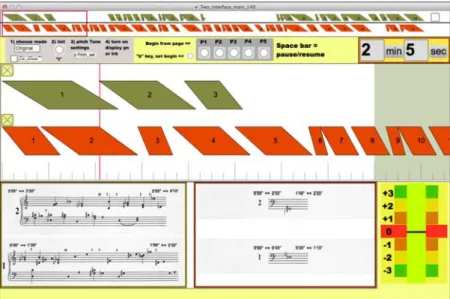
In previous work [8] we modeled these time brackets by parallelograms (see Figures 2 and 3) to build computer interfaces for interpretation assistance in the context of Cage’s Two5 _{(Fig. 2).}

Fig. 2. Cage’s Two5 _{main computer interface}

Over time ([9], [10], [11]), we realized that the shape used to represent time brackets, brought important information for the interpretation and musical analysis. The unusually long duration of this piece, 40 minutes, and the use of time brackets show that the temporal question, and its representation, is essential in the Number Pieces, in general, and in Two5 _{in particular.}

The computer interface whose use has become obvious, has created for us a climate of confidence in our relationship to the piece. Random encounters of synchronicity as

well as intervals bring unexpected situations…[12]

In the present text, we propose a general geometric study of these time brackets representations, while trying to make the link with their musical properties to improve the performance.

3 The Geometry of Time Bracket

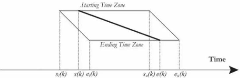
The first step in the process was to model a graphic representation of each part as a succession of musical events in time. For this purpose, the temporal structure of the piece has been represented as quadruples on a timeline. ("#($), "(($), )#($), )(($) ).

In order to place an event k on the timeline, time brackets are defined as quadruples to indicate the time span allocated to it. Each quadruple consists of two pairs. More precisely, each pair gives the interpreter lower and upper time bounds to start ("_#($), "₍($) ) and to end ()#($), )(($) ). Theses closed time intervals give to the

performer, a choice of the pair ("($), )($) ), where ("#($) ≤ "($) ≤ "(($) ) and

()_#($) ≤ )($) ≤ )₍($) ). One could choose the starting time ("($)), while performing and, then accordingly, the end time ()($)). This is the way one would employ when actually performing the work.

To obtain a graphic representation of each event in time we consider the quadruple: ("#($), "(($), )#($), )(($) )

where ("#($), "(($) ) is the Starting Time Zone and ()#($), )(($) ) the Ending Time Zone. As the two intervals have, in our case, a designed superposition, we prefer to

distinguish starting and ending zones by using two parallel lines (Fig. 3).

Fig. 3. Graphic representation for a generic time event

The graphic event obtained by connecting the four points has a quadrilateral shape. The height has no particular meaning. The starting duration +,($) is defined as the

difference: ( "(($) − "#($) ), which is the time span the performer has to start the

event. In the same way the ending duration +.($) will be the time span given to end

the event ( )(($) − )#($) ). In the general case, these values are not the same, and the

form we get is asymmetrical. When dealing with Cage’s Number Pieces, one generally has: +,($) = +.($), both durations are the same, and the figure to represent an event

is a trapezoid (Fig. 4). This is the case in the majority of the corpus we are treating. Special cases will be mentioned later on.

Starting Time Zone

sl(k) el(k) su(k) eu(k)

Ending Time Zone

Fig. 4. Graphic representation for a time event in Cage's Number Pieces

There is mostly an overlapping of the two time zones, ("#($), "(($) ) and

()#($), )(($) ) but it can happen that those are disjoined. We can define a variable

0($) where: "#($) + 0($) = )#($). In Cage's Number Pieces, 0($) depends generally

on the event duration. Thus, we don't have a big variety of forms. For example, in Five3_,

we have only 4 different time brackets sorts, for a total number of 131 events for the five instruments and 0($) =2₃+ ($) for all quadruples.

We make a distinction between a generic musical event and a real (or determined)

musical event. A real musical event is the one whose starting points (s) and end points

(e) are defined, that is, where there is a concretization of choice. One could represent this by a straight line from "($) to )($) (Fig. 5).

Fig. 5. A real music event represented by a straight line, joining the starting

to ending time zones

There are certain properties of a generic event that can easily be deduced from the trapezoidal graphic representation:

1. The starting or ending durations: +,($) or +.($) are a kind of a nominal duration

that Cage gives to an event.

2. The maximum duration, )(($) − "#($) = +456($), is the maximum length

(duration) an event can have.

3. The fact that, "(($) > )#($) means that we can choose a starting point s(k) placed

after the end, which leads to an empty musical event ∅ (an important idea of Cage: he often indicates that the artist can choose, all of, a part of, or nothing of the material placed at its disposal). In this case, s(k) > e(k).

Starting Time Zone

sl(k) el(k) su(k) eu(k)

Ending Time Zone

4. An alternative way to present a quadruple will be: ("#($), +,($), +.($), 0($) )

where 0($) is the value previously discussed. This representation can easily display the regularity in the time brackets construction (Fig. 6). It is easy to see that

+456($) =

(+,($) + +.($))

2 + 0($).

Fig. 6. An event represented as (;<(=), >;(=), >?(=), @(=) )

5. An implicit parameter that is important is the straight line’s slope of the concrete event (Fig. 5). This value is inversely proportional to the concrete event duration. The slope is strongly related to performance: it shows how much time the performer has for a particular event k. In regard to a wind instrument part, often only composed by held notes, knowledge of this parameter allows the artist to better manage his air capacity, in order to respect the composer’s indications. As far as the pianist is concerned, the slope gives some information that allows him to manage his interpretation with reference to the time indications. When the straight line of a concrete event is close to the vertical, the event will be short and concentrated.

The relationships of the generic events

Concerning the placement of two contiguous events k and k+1 we can define a variable A($), the gap between the elements k and k+1 where:

A($) = "#($ + 1) − )(($) (Fig. 7).

Fig. 7. C(=), The gap between the elements k and k+1

sl(k) sl(k+1) el(k) eu(k) el(k+1) eu(k+1) su(k) su(k+1) Time

k

_k+1

We will observe five typical placements of two contiguous events. 1. e > 0.

The two events are separated on the timeline. There is a minimum length of silence between the two events, which will probably be longer according to the choice of )($) and "($ + 1). In Five3 _{for example, we have events 1 and 2 of violin 2 separated}

by more than 8 minutes, or 3 minutes between events 6 and 7 of violin 1. Here the piece could also be considered from the point of view of the relative density of the musical elements. One should mention the global statistical approach done elsewhere [4] [5].

2. e = 0.

The two events are adjacent (Fig. 8).

Fig. 8. e = 0

Again, a gap may occur between the two events as the actual ending of event k: )($), and/or the actual starting of event k+1, "($ + 1) will differ from )(($), and

"#($ + 1) correspondingly. For example, Two5, trombone, events 21 and 22 (Fig. 9),

events 27 and 28.

Fig. 9. Two5_{, trombone, events 21 and 22}

sl(k+1)

eu(k)

Time

k

k+1

3. e < 0.

In this case, the performer’s opinion and attitude can determine the performance. There are many remarkable cases of interest in this situation; we could mention some cases that presently occur in Cage’s Number Pieces (Fig. 10). For example, Two5_,

trombone events 28 and 29, and piano events 6 and 7.

Fig. 10. e < 0, ;<(= + D) = ;E(=)

While performing event k, the player could start the event k+1 when not yet ending event k. We can encounter a superposition as shown in Fig. 11. For example, Two5_,

trombone events 37 and 38; piano events 9 and 10, events 12 and 13.

Fig. 11. e < 0, ;<(= + D) < ;E(=)

And even the same starting time for the two events: "#($ + 1) = "#($) (Fig. 12). For

example, Two5_{, piano, events 14 and 15 (Fig. 13).}

Fig. 12. e < 0, ;<(= + D) = ;<(=) su(k) sl(k+1) Time

k

k+1

k

k+1

k

k+1

Fig. 13. Two5_{, piano, events 14 and 15}

As the events have an order given by Cage, one may assume that the sequence of events is to be respected. But the performer may consider mixing the two events and choosing the respective ending times, )($) and )($ + 1).

In some case one has the configuration shown in Fig. 14. For example, Two5_,

trombone events 31 and 32, events 39 and 40.

Fig. 14. e < 0, ;<(= + D) < ;<(=)

This may be a mistake, in calculation or in printing. Again, without change the order of events, one could start with the event k, and continue with the event k+1, mixing or separating. Starting with the event k+1 would mean that mixing has to happen, or the event k, should be skipped, that an idea dear to Cage: the event k wouldn’t be performed.

The presentation of the time brackets as geometric figures and the variables we have defined lead to calculate some constants related to each of the instruments involved. The average filling rate (GHIII) gives an indication of how much a particular instrument is present during the piece. This value will be the ratio of the sum of all the events’ duration by the overall length of the work (Δ), where the event duration, +($), is the arithmetic mean between +,($) and +.($) (1).

GH

III =∑ +($)LM

Δ (1)

In the analog way, if we set: A(0) be the gap before the first event, and A(O) the gap after the last event n, the average silence rate (PHIII) will be the ratio of the sum of all the gaps between the events by the overall length of the work (2).

Time

k

k+1

sl(k)

PH

III =∑ A($)LQ

Δ (2)

These interesting values are based on the lengths of events, the gaps between them and their number, independent of the contents of the events.

If instead of using +($), the event duration, we consider +456($), then:

R +456($) + R A($) L Q = ∆ L TUM (3)

4 Musical Analysis Application

Table 1 shows the values for the 21 events of violin 1 in Five3_{, and the constants we}

just defined. The time values, onsets and durations, are defined in seconds.

Table 1. Data for Five3_{, first violin}

The following Table 2, compares these constants for the five instruments. We can observe how these two constants (GHIII VOW PHIII ) are strongly related to the presence of the instruments. For example, trombone will be more present, more active than the string instruments. One can see that PHIII may be negative. This occurs when many of the events are superposed (All cases with A < 0).

Table 2. Comparison values in Five3

#Events GHIII PHIII Violin 1 21 0.34 0.43 Violin 2 12 0.16 0.74 Viola 26 0.34 0.44 Violoncello 25 0.23 0.5

Trombone 47 0.74 -0.24

These values are clearly reflected in the form of the piece seen in the upper part of Fig. 15. We had implemented several models, some offline in “OpenMusic”1 _computer

aided composition software, and in a real-time “Max” software [8]. Fig. 15 presents a generic computer interface we are exploring, to perform most part of Cage’s Number

Pieces.

Fig. 15. Computer interface used for performing Five3

The medium part of this figure, displays one of the instruments chosen (here violin 1) and bottom part displays the musical score corresponding to the time (here 30 seconds after beginning). The global view displays a presentation of the entire duration of Five3_,

using the trapezoidal event representation. It allows the performer to have a global view of the piece at a glance. As Cage mention about the context-specific character of his time-bracket notation:

Then, we can foresee the nature of what will happen in the performance, but we can’t have the details of the experience until we do have it. [6]

This global representation enables another perspective of the piece. The printed score orients a natural local view. More than being a graphic representation for each time bracket, it allows us to identify similarities between generic musical events. Fig. 16, a detail from Fig. 15, presents the first ten minutes of the global representation of

Five3_.

1 _{“OpenMusic” is a software developed by Ircam by Gerard Assayag, Carlos Augusto Agon}

Fig. 16. The first ten minutes of the global representation in Cage’s Five3

In an analog way Table 3 presents GHIII _and PHIII constants for Two5_{, and Fig. 17 shows}

the global structure of the piece. One can clearly distinguish the difference in the presence of the two instruments.

Table 3. Comparison values in Two5

#Events GHIII PHIII Piano 29 0.33 0.15 Trombone 40 0.46 -0.14

Fig. 17. Two5 _{global structure}

5 Conclusions

At the present time we work to offer the musicians a way to approach other pieces from the same family, constructing a generic interface. The task may be somewhat complicated. The works called Number Pieces, share the same principal described earlier, but often contain particularities and exceptions in the instructions for performance. The interface then has to be adapted to cover these.

The interface is a substitute to the printed score. It reveals the structure of the work and provides the performer with the tool to achieve the “meditative concentration” needed. The few instructions given by Cage are integrated in the interface.

Considering the graphic representation, we presented above, our main goal was to find geometric properties and strategies to enhance the performance of these pieces through computer interfaces. John Cage’s works have been the target of our work for several years now. We have developed computer tools for the interface, and used it in practice. Both concerts and recordings have been the tests for the usefulness of the approach towards performance. The modeling process is transformed in a pragmatic analysis of the musical phenomena that leads us, step by step, to model some of Cage’s

concepts. Mentioning first the Concert for Piano and Orchestra (1957), an earlier work that has become important step of his output [7]. Followed by two of his number pieces for a small number of performers [8]. These works were also the object of a recording and performance sessions ([9], [10], [11]).

References

1. Haskins, R.: The Number Pieces of John Cage. DMA dissertation, University of Rochester (2004). Published as Anarchic Societies of Sounds, VDM Verlag (2009).

2. Chilton, J. G.: Non-intentional performance practice in John Cage's solo for sliding trombone, DMA dissertation, University of British Columbia (2007).

3. Pritchett, J.: The Music of John Cage, Cambridge University Press, Cambridge (1993). 4. Popoff, A.: Indeterminate Music and Probability Spaces: the Case of John Cage's Number

Pieces, MCM (Mathematics and Computing in Music) Proceedings, pp. 220--229. Springer Verlag (2011).

5. Popoff, A.: John Cage’s Number Pieces: The Meta-Structure of Time-Brackets and the Notion of Time, Perspectives of New Music Volume 48, Number 1, pp. 65—83 (Winter 2010). 6. Retallack, J.: Musicage: Cage muses on words, art, music, Wesleyan university Press, p. 182

(1996).

7. Sluchin, B., Malt, M.: Interpretation and computer assistance in John Cage’s Concert for piano and Orchestra (1957-58). 7th _{Sound and Music Conference (SMC 2010), Barcelona (21-24}

July 2010).

8. Sluchin, B., Malt, M.: A computer aided interpretation interface for John Cage’s number piece Two5_{. Actes des Journées d’Informatique Musicale (JIM 2012), pp. 211—218, Namur,}

Belgique (9–11 mai 2012).

9. Cage, J.: Two5_{. On John Cage Two}5 _{[CD]. Ut Performance (2013).}

10. Cage, J.: Music for Two. On John Cage, Music for Two [CD]. Ut Performance (2014). 11. Cage, J.: Ryoanji. On John Cage, Ryoanji [CD]. Ut Performance (2017).