HAL Id: halshs-00175051
https://halshs.archives-ouvertes.fr/halshs-00175051
Submitted on 26 Sep 2007HAL is a multi-disciplinary open access archive for the deposit and dissemination of sci-entific research documents, whether they are pub-lished or not. The documents may come from teaching and research institutions in France or abroad, or from public or private research centers.
L’archive ouverte pluridisciplinaire HAL, est destinée au dépôt et à la diffusion de documents scientifiques de niveau recherche, publiés ou non, émanant des établissements d’enseignement et de recherche français ou étrangers, des laboratoires publics ou privés.
Competition, Hidden Information and Efficiency: An
Experiment
Antonio Cabrales, Gary Charness, Marie Claire Villeval
To cite this version:
Antonio Cabrales, Gary Charness, Marie Claire Villeval. Competition, Hidden Information and Effi-ciency: An Experiment. 2006. �halshs-00175051�
IZA DP No. 2296
Competition, Hidden Information and Efficiency:
An Experiment
Antonio Cabrales Gary Charness Marie-Claire Villeval DISCUSSION P APER SERIES Forschungsinstitut zur Zukunft der Arbeit Institute for the Study September 2006Competition, Hidden Information
and Efficiency: An Experiment
Antonio Cabrales
Universidad Carlos III de MadridGary Charness
University of California, Santa BarbaraMarie-Claire Villeval
CNRS-GATE and IZA BonnDiscussion Paper No. 2296
September 2006
IZA P.O. Box 7240 53072 Bonn Germany Phone: +49-228-3894-0 Fax: +49-228-3894-180 Email: [email protected]Any opinions expressed here are those of the author(s) and not those of the institute. Research disseminated by IZA may include views on policy, but the institute itself takes no institutional policy positions.
The Institute for the Study of Labor (IZA) in Bonn is a local and virtual international research center and a place of communication between science, politics and business. IZA is an independent nonprofit company supported by Deutsche Post World Net. The center is associated with the University of Bonn and offers a stimulating research environment through its research networks, research support, and visitors and doctoral programs. IZA engages in (i) original and internationally competitive research in all fields of labor economics, (ii) development of policy concepts, and (iii) dissemination of research results and concepts to the interested public.
IZA Discussion Papers often represent preliminary work and are circulated to encourage discussion. Citation of such a paper should account for its provisional character. A revised version may be
IZA Discussion Paper No. 2296 September 2006
ABSTRACT
Competition, Hidden Information and Efficiency: An Experiment
We devise an experiment to explore the effect of different degrees of competition on optimal contracts in a hidden-information context. In our benchmark case, each principal is matched with one agent of unknown type. In our second treatment, a principal can select one of three agents, while in a third treatment an agent may choose between the contract menus offered by two principals. We first show theoretically how these different degrees of competition affect outcomes and efficiency. Informational asymmetries generate inefficiency. In an environment where principals compete against each other to hire agents, these inefficiencies remain. In contrast, when agents compete to be hired, efficiency improves dramatically, and it increases in the relative number of agents because competition reduces the agents’ informational monopoly power. However, this environment also generates a high inequality level and is characterized by multiple equilibria. In general, there is a fairly high degree of correspondence between the theoretical predictions and the contract menus actually chosen in each treatment. There is, however, a tendency to choose more ‘generous’ (and more efficient) contract menus over time. Competition leads to a substantially higher probability of trade, and that, overall, competition between agents generates the most efficient outcomes.JEL Classification: A13, B49, C91, C92, D21, J41
Keywords: experiment, hidden information, competition, efficiency
Corresponding author: Marie-Claire Villeval CNRS-GATE
93, Chemin des Mouilles 69130 Ecully
France
E-mail: [email protected]
1. INTRODUCTION
The theory of markets with asymmetric information has been a “vital and lively field of economic research” (2001 Nobel Prize committee) for decades. The classic ‘lemons’ paper (Akerlof 1970) illustrated the point that asymmetric information led to economic inefficiency, and could even destroy an efficient market. Since the seminal works of Vickrey (1961) and Mirrlees (1971), research on mechanism design has sought ways to minimize or eliminate this problem.1 In an environment with hidden information (sometimes characterized as adverse selection), each agent knows more about her2 ‘type’ than the principal does at the time of contracting. In the standard labor scenario, a firm hires a worker but knows less than the worker does about her innate work disutility. Other typical applications include a monopolist who is trying to price discriminate between buyers with different (privately known) willingness to pay, or a regulator who wants to obtain the highest efficient output from a utility company with private information about its cost.3
The fact that agents know their own ability levels while principals may not causes difficulties in contracting, as an agent may not choose the action that is in the best interest of the principal. If outcomes are related to actions, firms with complete information could design ‘first-best’ contracts that theoretically induce truthful revelation of types and generate economic efficiency by making the contract contingent on the outcome. However, in contracting under hidden information, the problem is how to induce the efficient action without being able to observe the agent’s true type; in this case, it is typically necessary to devise ‘second-best’
1
Applications include public and regulatory economics (Laffont and Tirole 1993), labor economics (Lazear 1999), financial economics (Freixas and Rochet 1997), business management (Milgrom and Roberts 1992), and development economics (Ray 1998).
2
contracts that lead to separation of types, but which are somewhat distorted and less than fully efficient.
Perhaps due to the complexity of business relationships, it is difficult to find support from field data for principal-agent theory. While there has been considerable theoretical work on contracts in recent decades, empirical tests of the theory have long remained scarce. Prendergast (1999)’s and Chiappori and Salanié (2003)’s surveys show that the econometrics of contracts has recently become a burgeoning field of research. The latter point however that a number of empirical tests suffer from selection and endogeneity biases. In addition, many papers use similar data because of a lack of data on contracts. These difficulties explain that only few empirical tests of the adverse selection problem are available in the literature (see notably Cawley and Philipson, 1999; Chiappori and Salanié, 2000; Dahlby, 1983; Dione and Doherty, 1994; Finkelstein and Poterba, 2000; Genesove, 1993; Puelz and Snow, 1994; Young and Burke, 2001). Given the difficulties inherent with field data in this area, laboratory experiments offer a complementary approach that offers some promise, since it is possible to isolate and vary the factors of interest while keeping all others constant.
We perform experiments designed to test the influence of competition on the management of hidden-information problems. This can be seen as a question of organizational or institutional design – what effects do different rules and markets have on performance and efficiency?4 We examine how differing degrees of relative bargaining power between principals and agents affect outcomes and efficiency when there is a problem of hidden information.
3
One-shot contracts are common in consumer transactions. In the public sector, government procurement is often conducted on a one-shot basis.
4
Although we use the standard static screening model, it is worth noting that Kanemoto and MacCleod (1992) examine the effect of competition in a dynamic environment and find that one obtains the first-best outcome if there is sufficient competition for workers, even with asymmetric information. Perhaps there is some empirical analog to this result in the static case.
Our approach is to systematically vary the type of competition present in the environment. In our benchmark case, each principal is matched with one agent of unknown type. In our second treatment, a principal can select one of three agents, while in a third treatment an agent may choose between the contract menus offered by two principals. Principals can choose to offer one of six feasible contract menus, which are held constant across our treatments; in turn, agents can select high or low effort, or reject the contract menu entirely and receive reservation payoffs. We derive the equilibrium predictions for each environment and include the induced contract menus for each treatment among the six feasible choices for the principal. We examine the outcomes in each treatment, ranking the institutions as a function of their relative efficiency, both in terms of effort and the probability of trade.
In this respect theory provides a first answer. To understand the theoretical efficiency ranking, it is important to realize that incomplete information in markets creates inefficiencies because the agents have a certain monopoly power. More precisely, they are the sole ‘owners’ of a valuable resource – information about their type. We first show from a theoretical point of view how different degrees of bargaining power between principals and agents, related to various degrees of competition in the market, affect outcomes and efficiency. In an environment where principals compete against each other to hire agents, inefficiencies remain. In contrast, in an environment where agents compete to be hired, efficiency improves dramatically and increases in the relative number of agents because competition reduces the agents’ informational monopoly power. However, this environment also generates a high inequality level and is characterized by multiple equilibria, which may have important behavioral implications in the field if people have social preferences such as inequality aversion.
Our experiment constitutes the first test of the impact of various competitive frameworks on the design of contracts in the presence of both heterogeneous agents and hidden information, and their subsequent efficiency. Our results are mostly supportive of the theory and the major implication is that the bargaining power directly affects the choice of contract menus. In comparison with environments in which there is either no competition or a competition among principals, our experiment finds that the institutional environment in which agents compete against each other the most efficient as far as we consider the contracting pairs.
Even though, in general, there is a fairly high degree of correspondence between the theoretical predictions and the contract menus actually chosen in each treatment, there is a tendency to choose more ‘generous’ (and more efficient) contract menus over time. We find that competition leads to a substantially higher probability of trade, and that, overall, competition between agents generates the most efficient outcomes. We observe a fairly high degree of separation of agents’ types in the choices made in response to the various contract menus; interestingly, with agent competition we observe the more able agents foregoing the option that would pay them more (if they are chosen), in order to signal their type by choosing the option that less able agents should never choose.5 Our data also show considerable evidence of changes in behavior over time, as participants learn what is effective and what is not.
The remainder of the paper is structured as follows: We review the relevant literature in section 2, and we describe our theoretical model and derive its predictions in section 3. Our experimental design and implementation are presented in section 4, with the results given in section 5. We discuss welfare and efficiency considerations in section 6, and conclude in section 7.
5
2. RELATED LITERATURE
Previous experimental studies on asymmetric information have typically examined the behavioral issues present with individual contracting with hidden action (also known as moral hazard), where effort is not contractible; these studies include Berg, Daley, Dickhaut, and O’Brien (1992), Keser and Willinger (2000), Anderhub, Gächter, and Königstein (2002), and Königstein (2001).6 They observe that contracts are usually more generous than theoretically predicted and some suggest adding an equity constraint to the standard participation and incentive-compatibility constraints in the design of optimal contracts. Charness and Dufwenberg (forthcoming) consider the hidden-action problem and find that cheap-talk statements of intent
(promises) help to achieve desirable outcomes (the Nash bargaining solution).
There is very little experimental work on hidden information and certainly no study considers the effect of competition. Lynch, Miller, Plott and Porter (1986) confirmed the existence of a market for “lemons” in experimental oral double auctions, and Holt and Sherman (1990) do so in posted–offer auctions. Experiments by Brandts and Holt (1992) and Banks, Camerer and Porter (1994), however, provide mixed evidence about the ability of subtle equilibrium refinements to predict players’ behavior in simple signaling games. DeJong, Forsythe, and Lundholm (1985) observe that the low quality/low price outcome is less frequent when the buyer cannot distinguish between a rip-off and bad luck. Cabrales and Charness (2004) study the static principal-agent problem with hidden information in the context of team
6
Other studies involving moral hazard include Bull, Schotter, and Weigelt (1987), who examine the incentive effects of piece rate and tournament payment schemes, and Nalbantian and Schotter (1997), who investigate group incentive contracts. Plott and Wilde (1982), and DeJong, Forsythe, Lundholm, and Uecker (1985) consider moral hazard problems with multiple buyers and sellers. Güth, Klose, Königstein, and Schwalbach (1998) consider a dynamic moral hazard problem where trust and reciprocity issues impede obtaining the first-best outcome.
production. They observe that when more equitable menus are proposed, rejection rates are less important and agents select actions according to their types. There are two studies of the dynamic contracting problem: Chaudhuri (1998) and Cooper, Kagel, Lo, and Gu (1999) study the problem of the ratchet effect, where the agent has an incentive to conceal her true type, as the principal may use this information to ratchet up the demands for performance in later periods. Nevertheless, principal-agent interactions in the field are frequently one-shot affairs; furthermore, if the principal could commit to an ex ante contract, it would be optimal to implement the one-shot problem in the dynamic setting.7
One might predict that different forms of competition should lead to different contract menus being selected, given the differences in the players’ bargaining power. However, results from the handful of experimental papers on the effects of unbalanced competition on the outcomes between firms and workers (or principals and agents) is somewhat mixed. Brandts and Charness (2004) find little difference in the gift-exchange outcomes according to whether there are more workers than firms or vice versa. Fehr, Kirchler, Weichbold, and Gächter (1998) show that an unbalanced market eliminates fairness when contracts are complete but not when they are incomplete. On the other hand, Roth et al. (1991) find that principals capture nearly the entire surplus when 10 agents compete in a “demand game” similar to the ultimatum game. Davis and Holt (1994) show that the ability of a buyer to switch between two sellers provides a strong incentive to develop reputation in a repeated game. In an ultimatum game with responders’ competition, Grosskopf (2003) observes that although the initial demands are similar, demands in the game with competition become higher over time than in the game with no competition. Finally, Fischbacher, Fong and Fehr (2003) demonstrate that the introduction of
7
even a little competition provokes large behavioral changes. A model combining heterogeneous social preferences with decision errors enables to predict most of the experimental evidence with various degrees of competition. Thus, it is not clear ex ante what effects unbalanced competition will have on the hidden-information problem, particularly in terms of economic efficiency.
3. THE MODEL
In this section we describe the theoretical model that serves as the basis for the experimental design. As a preview, we note that the case with competition between principals (more principals than agents) yields a Rothschild-Stiglitz type of solution, which is invariant to the number of agents and generally inefficient. On the other hand, the case of competition between agents is not invariant to the (relative) number of agents. The presence of more agents relaxes the binding incentive-compatibility constraint (for the high type), yielding a level of effort that decreases towards the efficient level with the number of agents. In the limit, the only relevant constraint for the high-type agent is the participation constraint. As a result, there are no inefficiencies.
Imagine that a firm needs one worker in order to be able to operate. The profits for the firm when it is operating are:
Π = e– w
where e, w are the effort levels and wages of the worker. Each worker has a utility function which depends on her type j ∈ {H,L}, which is her private information:
2 2 ) , (e w w k e uj = − j
where kH = 1 and kL = k > 1. That is, the high type of agent has a lower cost of effort than the
lower type. Thus, only the individual agent knows j, but e is observable and contractible. From the utility functions of the principal and the agents we have that the first-best effort levels are:
{
H L j k e j j , , 1 ˆ = ∈}
(1) We call e ˆ j the efficient level of effort.8 If we denote by U the outside option of the worker (which we assume for simplicity to be type-independent) we can induce optimal effort, with:{
H L}
j k U w j j , , 2 1 ˆ = + ∈If the (independent) probability that an agent is a high or low type is denoted respectively by or , then the expected (optimal) profits for the principal are given by:
H p L p U k p k p H H L L E = + − Π 2 2
In order to make some comparisons across treatments we hold this first-best contract fixed in all the treatments. However, the second-best optimal equilibrium contracts, when the types are private information of the agents, depend on the structure of the market, which is our treatment variable. Then the equilibrium contract menu in the Benchmark (one principal-one agent) treatment results from the solution of the maximization program:
8
This is an appropriate terminology because in all the Pareto-efficient allocations of this problem (with complete information) the level of effort is always . This is so because of the quasi-linearity of the utility function of the agents, a common assumption in this field. Thus, the Pareto-efficient allocations only differ in the wages and profits of the principal and agent.
ˆ
) ( ) ( max , , , ,wLeH eL H H H L L L H w w e p w e p − + − subject to wH− kH 2 (eH) 2≥ U (IRH) wL−kL 2 (eL) 2 ≥ U (IRL) 2 2 ) ( 2 ) ( 2 L H L H H H e k w e k w − ≥ − (ICH) ) (IC ) ( 2 ) ( 2 L 2 2 H L H L L L e k w e k w − ≥ −
where (IRj) and (ICji) are respectively the individual rationality and incentive compatibility
constraints of an agent of type j ∈ {H,L}. As usual in these problems, it turns out that the active constraints in the optimal solution are (IRL) and (ICH), so that the solution is:
eHB = 1 kH =1; eL B = pL kL−kH(1− pL)= 1 kL +1−pL pL (kL−kH) ; wLB =U+ kL 2 (eL B )2; wHB =1 2+wL B −1 2(eL B )2 (2)
The high type of agent provides the ‘efficient’ level of effort and obtains utility above U . These informational rents (rents are defined here as the utility an agent gets above her reservation utility) are equal to:
2 ) ( 2 1 2 1 B L L B H e k U w − − = − (2e)
The effort of the low type of agent is ‘inefficiently’ low and she obtains no rents, because she is held to the reservation value (the (IRL) constraint is binding). This is the subgame-perfect
equilibrium of this game.
Assume now that the each principal is matched with 3 agents (this is the Excess Agent treatment). Then an equilibrium contract menu results from the solution of a slightly different maximization program. Given that high types are “harder-working” (they have a lower disutility of effort) they cost less per unit of output. Thus when any of the matched agents chooses the contract designed for the high type, the principal always chooses her. If more than one agent chooses the high contract, the principal chooses randomly among those selecting the high contract.9 ) ( ) )( 1 ( max 3 3 , , , ,wL eH eL L H H L L L H w w e p w e p − + − − subject to wL−kL 2 (eL) 2 ≥ U (IRL) (1− pL)2 3 + 2 (1− pL) pL 2 + pL 2 ⎛ ⎝ ⎜ ⎞ ⎠ ⎟ wH − kH 2 (eH) 2 ⎛ ⎝ ⎜ ⎞ ⎠ ⎟ + 1−(1− pL) 2 3 − 2 (1− pL) pL 2 − pL 2 ⎛ ⎝ ⎜ ⎞ ⎠ ⎟ U ≥ pL3 3 wL− kH 2 (eL) 2 ⎛ ⎝ ⎜ ⎞ ⎠ ⎟ + 1− pL 3 3 ⎛ ⎝ ⎜ ⎞ ⎠ ⎟ U (ICH)
The (ICH) can also be written
U q e k w q e k wH H H L H ( L) (1 ) 2 ) ( 2 2 2 ⎟+ − ⎠ ⎞ ⎜ ⎝ ⎛ − ≥ − (ICH)
where 2 2 3 2 ) 1 ( 2 3 ) 1 ( 3 L L L L L p p p p p q + − + −
= . The solution is now:
2 2 3 3 ) ( 2 1 2 1 ; ) ( 2 ; ) ( ) 1 ( 1 ; 1 1 EA L EA L EA H EA L L EA L H L L L L EA L H EA H e w w e k U w k k q p p k e k e − + = + = − − + = = = (3)
The effort of the low type of agent in the EA treatment eLEA is closer to the efficient effort (e ˆ L) than
that in the Benchmark treatment (eLB). To see this note first that both eLEA and eLB are smaller than
L L
k
eˆ = 1 , but we will now show eLEA >eLB , so that the distortion is lower in EA than in B:
1 ) 1 ( ) ( 1 1 ) ( ) 1 ( 1 2 2 3 3 < − ⇔ − − + = > − − + = q p p k k p p k e k k q p p k e L L H L L L L B L H L L L L EA L 1 3 ) 1 ( 3 ) 1 ( 2 ) 1 ( 2 3 ) 1 ( 3 ) 1 ( 2 ) 1 ( 2 3 ) 1 ( 3 ) 1 ( ) 1 ( 2 2 2 2 2 2 2 3 2 2 2 2 ≤ − − < + − + − − = + − + − − = − L L L L L L L L L L L L L L L L L L p p p p p p p p p p p p p p p p q p p (3’)
The reason for this enhanced efficiency is that the principal distorts the low agent in order to lower the rents to the high agent. To see this, note that the informational rents in the Benchmark treatment (equation 2e) are increasing in , so the principal prefers to lower (thus reducing efficiency) in order to get higher profits. But in the EA treatment there is a competitive pressure on the high types, the presence of other high types that makes this less necessary. In fact, it is easy to check that in the general model where the principal confronts n agents, the difference
B L
e eLB
9
between the equilibrium and the efficient level of effort for the low type goes to zero as n goes to infinity.
Nevertheless, there is an additional problem with this treatment. We have found the equilibrium by assuming that the high types assume that other high types choose the high contract. But that is not the unique equilibrium here. In the second stage, where a menu is offered, it is also possible that all agents, both high and low, select the low option for the menu. If all agents are choosing the low option, it is indeed a best response to choose low for all of them. But in this case, it need not be optimal to propose the menu of contracts specified in (3). In the design of the experiment we provide another menu, which is the equilibrium under the assumption that whenever there is multiplicity of equilibria in the second stage, the worst equilibrium for the principal is selected. The equilibrium menu in that case would solve:
max
wH,wL,eH,eL(1
− p
L 3)(e
H− w
H)
+ p
L3(e
L− w
L)
subject to wL−kL 2 (eL) 2 ≥ U (IRL) (4) U e k w e k wH H H L H L 3 2 ) ( 2 3 1 ) ( 2 2 2 ⎟+ ⎠ ⎞ ⎜ ⎝ ⎛ − ≥ − (ICH)where the incentive constraint now ensures that it is dominant to choose the high option for a high type (thus she will do it independently of what other individuals of her type are doing). Choosing the high contract when the low contract gives a higher payoff makes sense to reduce competition from other workers. In fact the ‘attractiveness’ of the high contract increases with the probability that a competing worker also chooses the high option. So the worst-case scenario for the principal is when no competitor chooses the high contract. If even in that case a high
type should choose the high over the low contract, then it is dominant for a high type to choose the high option, and that is exactly what the ICH constraint in equation (4) does.
Finally, we also have a treatment where several principals compete for one agent. In that case, the equilibrium of the game is such that the principals make zero profits for each type of contract, the low agent gets an undistorted contract and the high agent is held to his Incentive Compatibility constraint (see e.g. Mas-Colell, Green and Whinston, 1995, ch.14D).
L H EP H L EP L EP L EP L EP H EP H k k e k e w e w e 1 2 ; 1 ; ; − = = = = (5)
where eHEP comes from the Incentive constraint for the high type which solves
( )
2( )
2 2 1 2 1 EP L H EP L EP H H EP H k e w k ew − = − which from (5) can be rewritten as:
( )
1( )
2 2 1 0 2 1 1 2 1 2 2 2 2 2 = ⎟⎟ ⎠ ⎞ ⎜⎜ ⎝ ⎛ − + − ⇔ ⎟⎟ ⎠ ⎞ ⎜⎜ ⎝ ⎛ − = − L H L EP H H EP H L H L EP H H EP H k k k e k e k k k e k e , which leads to L H L H H L L H H H EP H k k k k k k k k k k e 1 1 1 2 1 2 4 8 4 2 2 2 2 − = ⎟⎟ ⎠ ⎞ ⎜⎜ ⎝ ⎛ − + = + − + = .We implemented the theoretical model in our experiment by choosing a single set of six menus allowable in all contracts. For the parameter values kL =2, kH =1, pL =1/2, equation (3)
leads to menu 1, equation (4) induces menu 2, equation (2) leads to menu 3, and equation (5) induces menu 6. We provide the details of these mappings into experimental payoffs in section 3. In addition we chose two non-equilibrium menus, in order to provide a richer contractual environment. Menu 4 is similar to menu 3, but has a little more effort for the low type, and
respects the IC constraint for the high type. Menu 5 is fully efficient, for both the high and the low types.
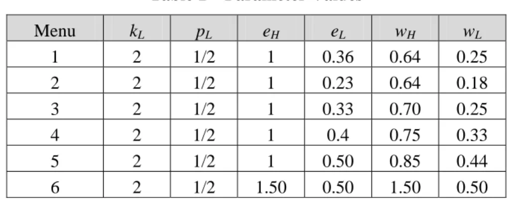
The values for the parameters in the six permitted contract menus are shown in Table 1. Each menu consisted of a choice of two (enforceable) effort levels and payments that depend on the type of agent involved; if neither choice seems attractive to the agent, she can veto the contract menu. We chose kL = 2 for all menus, in order to give relatively large rents to the high type
(under her preferred contracts). The parameters, efforts, and wages for the different menus in the experiment are summarized below:
Table 1 – Parameter Values
Menu kL pL eH eL wH wL 1 2 1/2 1 0.36 0.64 0.25 2 2 1/2 1 0.23 0.64 0.18 3 2 1/2 1 0.33 0.70 0.25 4 2 1/2 1 0.4 0.75 0.33 5 2 1/2 1 0.50 0.85 0.44 6 2 1/2 1.50 0.50 1.50 0.50
One of the criticisms of models of contract design with hidden information is that the contract menus are more ‘complex’ than one observes in reality. In an environment like ours, these often employ a nonlinear structure and a very large number of possible choices of pairs of wages and efforts. Using a continuous strategy space would be quite complicated to design for the principal, and even the choice of the agent would not be simple without adding much insight; this would also make the data analysis problematic. While we have selected a very simple structure (only two types), we feel that a ‘simple’ menu can serve as an approximation for a full schedule. As Wilson (1993) points out (p. 146) in a representative example: “The firm’s profits
from the five-part and two-part tariffs are 98.8% and 88.9% of the profits from the nonlinear tariff.”
4. EXPERIMENTAL DESIGN
We conducted three different treatments, which differed according to the numbers of principals and agents in the treatment. In our Benchmark (B) treatment, there were 10 principals and 10 agents in each session. In the Excess Agents (EA) treatment, there were four principals and 12 agents, while in the Excess Principals (EP) treatment, there were 12 principals and six agents.10 In all cases, there were equal numbers of high (H) agents and low (L) agents and this was made common knowledge among the participants. In order to observe roughly similar numbers of observations (matches) in each treatment, we conducted four sessions of the EA treatment, three sessions of the EP treatment, and two sessions of the B treatment. Each session consisted of 40 periods of play to allow for possible learning dynamics, with random and anonymous re-matching after every period. The re-matching procedure was common information to the participants. The organization of our sessions is summarized in Table 2.
Table 2 – Treatments and sessions
Participants per session
10
We chose 3 agents per principal in the EA treatment because the theoretical model shows that the distortion between the efficient level of effort and the equilibrium effort reduces in the number of competing agents; in addition, it increases the probability to be matched with at least one high agent. In the EP treatment, we chose to match two principals with one agent because the theoretical predictions are not sensitive to the size of the competing pool.
Participants per session Treatment
Principal s
H-agents L-agents Sessions Periods Observations Benchmark 10 5 5 2 40 800 Excess Agent 4 6 6 4 40 640 Excess Principal 12 3 3 3 40 720
Total 72 43 43 9 - 2160
The sessions were conducted at the Groupe d’Analyse et de Théorie Economique (GATE), CNRS, France. The subjects were recruited from undergraduate courses in local Engineering and Business schools. Some of the subjects had participated in previous experiments, but all of the subjects were inexperienced in this particular type of experiment. No subject participated in more than one session of the study. On average, a session lasted 60 minutes, including initial instructions and payment of subjects. The experiment was computerized using the REGATE program developed at GATE (Zeiliger, 2000).
The participants were privately informed of their role; agents were also informed of their type. One’s role and/or type were kept constant throughout the session. The participants also knew that there were the same number of low type and high type agents in the room. In our B treatment, the “proposer” (principal) first makes a selection from among the six “offers” (feasible contract menus). The “responder” (agent) is informed of this choice, and then selects “option X” (high contract), “option Y” (low contract), or rejects the contract menu. Each person then learns his or her payoff and play then continues on to the next period. The sequence in the
EA treatment is similar, except that the principal is informed of the options chosen by each of the
three agents and then selects one of these agents. No agent is informed about the choices of the two other agents. The EP treatment has the same sequence as the B treatment, with the proviso that an agent can accept at most one offer from the two principals with whom she is paired.
When both principals make the same offer, the agent chooses at random between the two principals if she is willing to accept the offer. The principal is not informed of the offer of the other principal.
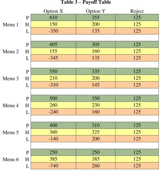
We used the parameter values in Table 1 to generate experimental payoffs for the feasible contract menus. We first derived the payoffs from these parameters to three decimals and then multiplied these by one thousand. We next rounded these payoffs to the nearest multiple of 5. In the case of the principals, we added 250 to each of the non-rejection payoffs; this reflects the notion that setting up the firm requires some capital, and the minimum level of revenues that are needed to recoup the cost of capital is 250. In the case of the agents, we added 10 to each non-rejection payoff, in order to provide some minimal separation (avoiding indifference) between the payoff for a low agent who accepts the least favorable offer and her payoff from rejecting the contract menu in its entirety.11 Unmatched principals or agents received 125 points in the period. This process leads to Table 3 that was distributed to the subjects to help them to make their decisions (except that the term “menu” was replaced by that of “offer”).12.
We used a conversion rate of 100 points for each Euro. At the end of each session, we selected (at random) four of the 40 periods for actual payment. In this way, we avoided possible income effects from having already accumulated a known amount of financial remuneration in the session. The average payoff was 14.9 Euros in the Benchmark treatment, and 13.5 Euros in both the Excess Agent and the Excess Principal treatments; on average the principals received 17 Euros, the high agents 13 Euros and the low agents 10 Euros, including a 4 Euro show-up fee.
11
As it happens, we inadvertently added 20 points to the L payoffs from option Y with menu 4. Perhaps this turns out to be useful for testing what is needed to obtain efficiency. The reason is that even with this extra kick, the B treatment is least efficient once rejections are considered. Thus, there is an argument that competition between agents is good for efficiency because it reduces informational rents, both in theory and in practice. And that
Table 3 – Payoff Table
Option X Option Y Reject P 610 355 125 Menu 1 H 150 200 125 L -350 135 125 P 605 305 125 Menu 2 H 155 160 125 L -345 135 125 P 550 335 125 Menu 3 H 210 200 125 L -310 145 125 P 500 350 125 Menu 4 H 260 230 125 L -240 160 125 P 400 310 125 Menu 5 H 360 325 125 L -140 200 125 P 250 250 125 Menu 6 H 385 385 125 L -740 260 125
5. EXPERIMENTAL RESULTS
An overview of our experimental results is that we find substantial treatment effects in our sessions, with large differences in the contract menus offered and accepted, substantially in line with the equilibrium predictions. The menus that are offered (and accepted) evolve over time. In general, rejections and competition drive behavior. We first give descriptive statistics
principal competition enhances efficiency as it reduces the envy-driven rejections that hurt efficiency in the benchmark.
12
for principal behavior and agent behavior, supplemented with charts. We then consider the determinants of such behavior, providing statistical tests and regression analysis.
4.1 Descriptive statistics Principal behavior
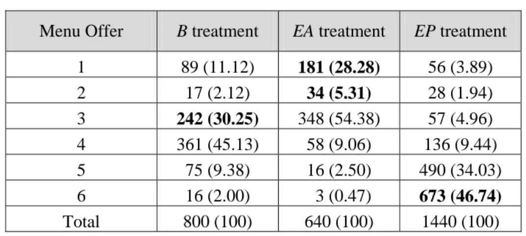
While there is certainly some heterogeneity present among the principals, we do observe some clear patterns and differences for the menus chosen in each treatment. We list the menus offered in each treatment in Table 4.
Table 4 – Menus offered, by treatment
Menu Offer B treatment EA treatment EP treatment
1 89 (11.12) 181 (28.28) 56 (3.89) 2 17 (2.12) 34 (5.31) 28 (1.94) 3 242 (30.25) 348 (54.38) 57 (4.96) 4 361 (45.13) 58 (9.06) 136 (9.44) 5 75 (9.38) 16 (2.50) 490 (34.03) 6 16 (2.00) 3 (0.47) 673 (46.74) Total 800 (100) 640 (100) 1440 (100)
Note: Equilibrium menus are in bold. Percentages are in parentheses.
The EA treatment has the ‘lowest’ contract menus (the ones most favorable to the principal), the
EP treatment has the ‘highest’ menus (the ones most favorable to the agents), and the B
treatment features intermediate menus. There is some support for the equilibrium predictions, as 30% of the menus offered in the B treatment, 34% of the menus offered in the EA treatment, and 47% of the menus offered in treatment EP are equilibrium menus (menus 1 and 2 with EA, menu 3 with B, and menu 6 with EP). However, menu 4 is the most common choice in the B treatment and menu 3 is the most common choice in the EA treatment.
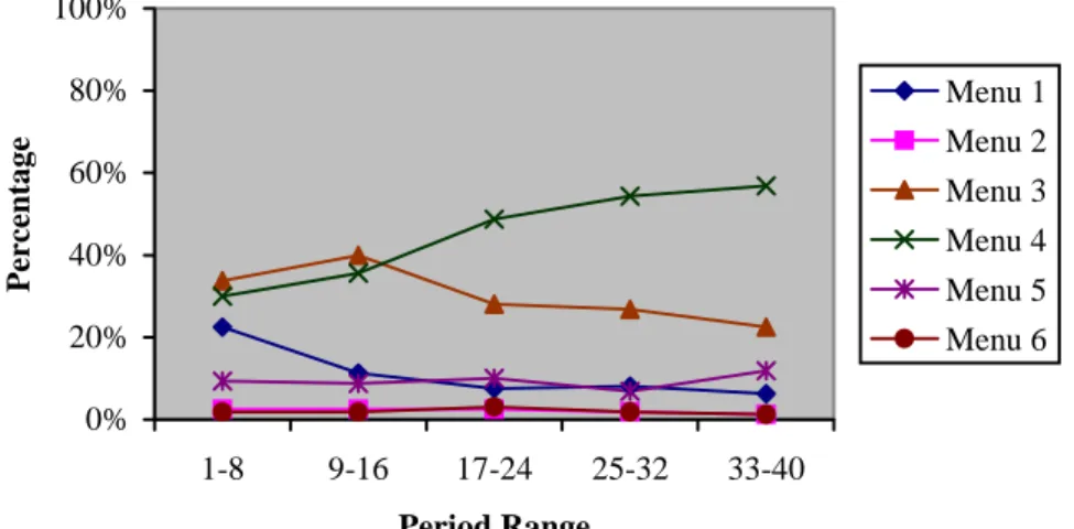
As menu 3 has a more egalitarian distribution than menu 1 (EA treatment) and also provides greater efficiency (higher total payoffs), one might suspect that social preferences such as those expressed in the Charness and Rabin (2002) model play a role here; a similar comment applies vis-à-vis menu 4 and menu 3 (B treatment). However, to the extent that these represent social preferences on the part of the principals, we should expect to see these choices from the beginning. Instead, the menus offered evolves over time, as can be seen in Figures 1-3.
Figure 1: Menu Offered over Time, Benchmark
0% 20% 40% 60% 80% 100% 1-8 9-16 17-24 25-32 33-40 Period Range Percentage Menu 1 Menu 2 Menu 3 Menu 4 Menu 5 Menu 6
Figure 2: Menu Offered over Time, EA
0% 20% 40% 60% 80% 100% 1-8 9-16 17-24 25-32 33-40 Period Range Percentage Menu 1 Menu 2 Menu 3 Menu 4 Menu 5 Menu 6
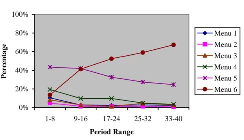
Figure 3: Menu Offered over Time, EP 0% 20% 40% 60% 80% 100% 1-8 9-16 17-24 25-32 33-40 Period Range Percentage Menu 1 Menu 2 Menu 3 Menu 4 Menu 5 Menu 6
In each of these treatments, there is some distribution across menus in the initial periods, but we typically see that two menus comprise the great majority of the menus offered thereafter in each treatment. In every case, it is the ‘higher’ menu that grows in frequency over time. Thus, it seems that some other force is inducing principals to choose more generous menus over time, even though principals’ social preferences may perhaps account for some of the generous menu choices. In every treatment, one menu predominates in the last group of periods, averaging about 60% of all menus offered (although there is a dip in favor of the equilibrium menu in EA).
While we postpone an in-depth analysis of the determinants of the contract menus offered by principals, Table 5 below shows the ex post profitability of these offers in our treatments;
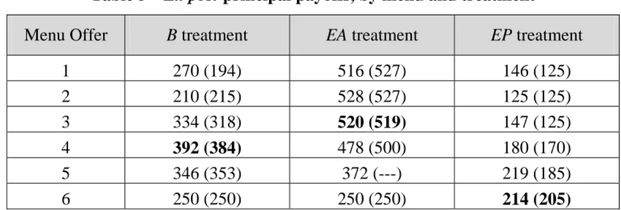
It is clear that the profitability of a particular contract menu depends greatly on the competitive environment. Menus 1 and 2 yield highest profits for the principal in the EA treatment, but generate low profits in the B and EP treatments. Similarly, menu 6 is quite unattractive for the principal in the EA and B treatments, but provides nearly the best profits in the EP treatment (and the best in the final periods). Overall, we observe a good correspondence
between the most frequent offers made and their profitability; thus, to a large extent, it seems that principals are influenced by considerations of their own profits.
Table 5 – Ex post principal payoffs, by menu and treatment
Menu Offer B treatment EA treatment EP treatment
1 270 (194) 516 (527) 146 (125) 2 210 (215) 528 (527) 125 (125) 3 334 (318) 520 (519) 147 (125) 4 392 (384) 478 (500) 180 (170) 5 346 (353) 372 (---) 219 (185) 6 250 (250) 250 (250) 214 (205)
Note: The most frequent menus are in bold. Payoffs for the last eight periods are in parentheses.
Agent behavior
The menus accepted by the agents naturally mirror the menus that were offered; however, there are some substantial differences, due primarily to rejections in the B treatment and selection pressures in the EP treatment. More favorable menus are more likely to be accepted in the B treatment, with 142 rejections of the 800 contract menus offered. The acceptance rate is 90% for menu 4, 75% for menu 3, but only 61% for menu 1. In addition, less favorable menus are not likely to be selected by agents in the EP treatment although rejections of offers from both principals occurred only twice. The punishment for offering an unfavorable contract menu is simply that no agent will select it. Menus 1 to 3 are only accepted about 5% of the time; in fact, these menus were never accepted in the final eight periods, and menu 4 was only accepted twice out of the 144 times it was offered in these periods. Finally, rejections in the EA treatment are not actually costly for the principal, since an offer has always been accepted by at least one agent.
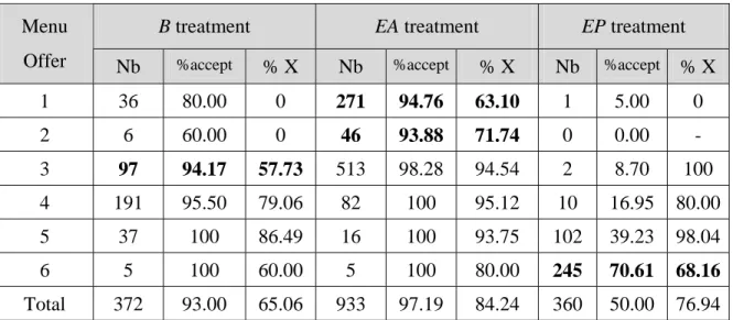
We summarize agent behavior by listing the number of accepted menus (column 1), the rate of acceptance (column 2), and the proportion of X option chosen (column 3) in each treatment in Table 6 for the high agents and Table 7 for the low agents.
Table 6 – High agents' choices, by treatment
B treatment EA treatment EP treatment
Menu
Offer Nb %accept % X Nb %accept % X Nb %accept % X 1 36 80.00 0 271 94.76 63.10 1 5.00 0 2 6 60.00 0 46 93.88 71.74 0 0.00 - 3 97 94.17 57.73 513 98.28 94.54 2 8.70 100 4 191 95.50 79.06 82 100 95.12 10 16.95 80.00 5 37 100 86.49 16 100 93.75 102 39.23 98.04 6 5 100 60.00 5 100 80.00 245 70.61 68.16 Total 372 93.00 65.06 933 97.19 84.24 360 50.00 76.94
Table 7 – Low agents' choices, by treatment
B treatment EA treatment EP treatment
Menu Offer
Nb %accept % X Nb %accept % X Nb %accept % X
1 18 40.91 11.11 212 82.49 1.42 4 11.11 0 2 2 28.57 0 47 88.68 0 0 0.00 0 3 85 61.15 2.35 446 85.44 0 2 5.88 0 4 134 83.23 2.98 92 100 0 18 23.38 0 5 36 94.74 5.56 32 100 0 99 43.04 0 6 11 100 9.09 4 100 0 235 72.09 0 Total 286 71.50 3.85 833 86.77 0 358 49.72 0
Note: Equilibrium menus are in bold.
We do see that the rejection rate for low agents is always much higher than the rate for high agents, more than four times as high in both treatments B and EA. When they accept an offer, low agents rarely chose option X, which would generate negative earnings. The behavior
of high agents is more complex. Note that option X pays more than option Y for high types with menus 3-5, but option Y pays more with menus 1 and 2. In addition, both options give the same payoff to the high type with menu 6. In the EP treatment, high agents nearly always maximize own payoffs (356 of 360 non-rejections). While they also do so with menus 1, 2, 5, and 6 in treatment B, we observe a substantial proportion of option-Y choices with menus 3 and 4 (42% and 21% of the non-rejection choices, respectively).
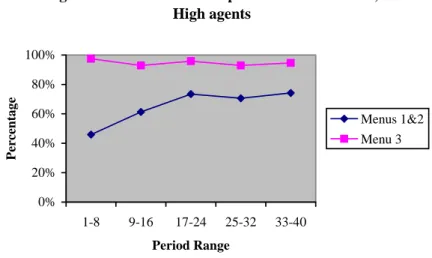
In the EA treatment, recall that agents’ choices are known to the principals prior to selecting an agent, so that agents must compete in their choices to be selected. High agents do maximize own profits with menus 3-5, since this maximization also coincides with maximizing the profits for the principal. However, with menus 1 and 2, an agent who myopically chooses option Y runs the risk that his principal will not select him by if another agent has chosen option X. Since some agents appear to realize this, we observe that 64% of the high agents choose option X when accepting menus 1 or 2. Figure 4 shows that high agents appear to be learning to do so over time, as this likelihood increases during the first half of the sessions.13 We also chart menu 3 for comparison, to show a ‘best-case scenario’ for the X option, since a high agent trying to compete should always choose it; note the lack of a time trend.
13
An indirect consequence of this pattern is that principals in the EA treatment are increasingly successful in obtaining option X in response to menu 1 or menu 2. Overall, option X was obtained 67% of the time in response to these menus; this proportion was 63% during the first 20 periods and 72% during the last 20 periods.
Figure 4: Likelihood of X Option over Time in EA, High agents 0% 20% 40% 60% 80% 100% 1-8 9-16 17-24 25-32 33-40 Period Range Percentage Menus 1&2 Menu 3
As a consequence of these decisions, the proportion of high agents actually recruited is larger in EA (81%) than in B (57%). While in B this distortion of the initial distribution of the population reflects the higher frequency of rejections of offers by low agents, in EA this reflects the process of selection related to the competitive environment. In EP, the proportion of high agents (50.14%) corresponds roughly to the initial distribution of the population since almost all the agents accept an offer. Regarding the evolution over time of the proportion of high agents, the selection process does not take a long time before being fully operative in EA, whereas there is almost no evolution in B. The percentage of high type among the agents recruited in EA rises from 71% in periods 1 to 8 up to 87% in periods 9 to 16 and stays above 81% in the following periods, whereas the proportion stays between 55 and 57% in B throughout the game.
4.2 Regression analysis
It appears that there are substantial and significant differences in both principal and agent behavior across treatments. We now turn to multiple-regression analysis of the determinants of the observed behavior, first considering the menus offered by principals.14 In order to
14
We also performed nonparametric Mann-Whitney rank-sum tests, with both session-level and individual-level data (see Appendix B). These tests find that the average menu offered is lowest in the EA sessions and highest in
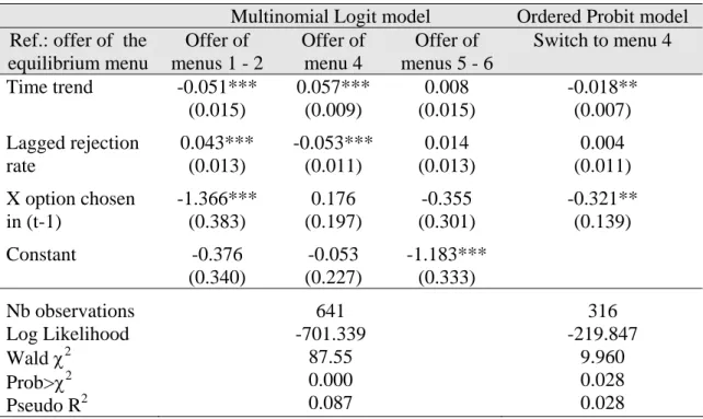
disentangle the motivations underlying offers of the different categories of menus, we estimate multinomial logit models with robust standard errors, in which the reference category is the offer of the equilibrium menu. To better understand the choice of the most frequent menu that is not necessarily the equilibrium one, we also estimate ordered probit models with robust standard errors in which the switch to the most frequent menu offer is the dependent variable, equal to +1 if the menu increased, 0 if unchanged, and -1 if it decreased. In all the regressions, we include a time trend to identify a possible evolution over time. The first three columns of Table 8 presents the results of the multinomial logit model and the fourth column the results of the ordered probit model for the contract menus chosen in the B treatment.
the EP sessions. They also indicate that rejection rates of menus below 4 are significantly higher in the B than in the EA treatments and that high agents in B are more likely to choose option X in response to menus 1 and 2 than in
EA, the reverse being true for menu 3. Overall, they show that the proportion of high agents is higher in EA than in
Table 8: Determinants of the choice of menus in the Benchmark Treatment
Multinomial Logit model Ordered Probit model Ref.: offer of the
equilibrium menu Offer of menus 1 - 2 Offer of menu 4 Offer of menus 5 - 6 Switch to menu 4 Time trend Lagged rejection rate X option chosen in (t-1) Constant -0.051*** (0.015) 0.043*** (0.013) -1.366*** (0.383) -0.376 (0.340) 0.057*** (0.009) -0.053*** (0.011) 0.176 (0.197) -0.053 (0.227) 0.008 (0.015) 0.014 (0.013) -0.355 (0.301) -1.183*** (0.333) -0.018** (0.007) 0.004 (0.011) -0.321** (0.139) Nb observations Log Likelihood Wald χ2 Prob>χ2 Pseudo R2 641 -701.339 87.55 0.000 0.087 316 -219.847 9.960 0.028 0.028
Note: Robust standard errors in parentheses; ***, and ** denote two-tailed statistical
significance at the 1%, 5%, and 10% level, respectively.
Menus 1 and 2 are chosen less frequently over the course of the sessions, while menu 4 is increasingly preferred to menu 3 in the latter periods of the sessions.15 The offer of very generous menus (11% of offers) does not follow a clear trend.
A principal who experiences a high proportion of rejections of his previous offers is more likely to offer menus 1-2 and less likely to offer menu 4. This may suggest some inertia in the motivations driving behavior. Indeed, a principal who is driven by social preferences makes more generous offers, experiences fewer rejections, and is encouraged to continue to offer generous menus. Moreover, an agent choosing the X option in the previous period (which never occurs in reaction to menus 1-2) strongly decreases the likelihood of menu 1-2 being chosen by the principal. This makes sense because offering these menus would induce both types to switch
to the low option. The ordered probit regression regarding switching from any menu to the most frequent menu 4 indicates that such a switch is more frequent at the beginning of the game. It is less likely if the agent has chosen the X option in the previous period. It shows no significance for whether the principal has experienced a high proportion of rejections in the past. In contrast, a similar regression in which the lagged option is replaced by the rejection of the menu offer in the previous period (not reported here) indicates that a rejection strongly favors such a switch. Overall, these regressions suggest that offering a more generous menu than the equilibrium is driven by the experience of recent rejections and the selection of low-type agents, whereas offering very generous menus (5 or 6) does not depend on any of these variables, suggesting a preference for more egalitarian outcomes.
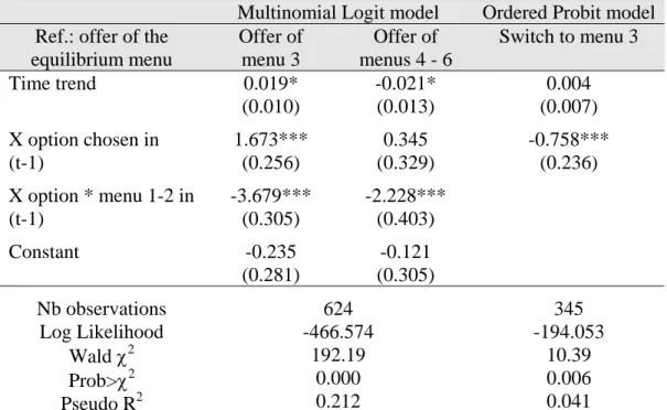
Table 9 presents the results for the menus chosen in the EA treatment. In the first two columns, we pool together the offers of menus 4 to 6 since they represent only 12% of the observations. The third column displays the results of the ordered probit model in which the switch to the most frequent menu 3 is explained. In contrast with the previous regression, we do not include the lagged rejection rate as an independent variable since all the contracts are accepted.
15
Table 9: Determinants of the choice of menus in the Excess Agent Treatment
Multinomial Logit model Ordered Probit model Ref.: offer of the
equilibrium menu Offer of menu 3 Offer of menus 4 - 6 Switch to menu 3 Time trend X option chosen in (t-1) X option * menu 1-2 in (t-1) Constant 0.019* (0.010) 1.673*** (0.256) -3.679*** (0.305) -0.235 (0.281) -0.021* (0.013) 0.345 (0.329) -2.228*** (0.403) -0.121 (0.305) 0.004 (0.007) -0.758*** (0.236) Nb observations Log Likelihood Wald χ2 Prob>χ2 Pseudo R2 624 -466.574 192.19 0.000 0.212 345 -194.053 10.39 0.006 0.041
Note: Robust standard errors in parentheses; *** and * denote two-tailed statistical significance
at the 1% and 10% level, respectively.
Menu 3 is chosen more frequently over time (we know from an alternative regression that this is particularly the case in periods 17-32,significant at 1%), whereas the frequency of menus 4-6 decreases (especially in the final eight periods with a coefficient significant at the 5% level). If the X option was chosen in the previous period in response to the offer of the equilibrium menu, this decreases the likelihood of non-equilibrium menus being offered; this makes sense, since the X option leads to a higher payoff for the principal, and so there is less motivation to offer a more generous menu. On the other hand, if the X option was chosen in the previous period (in reaction to whichever offers), this increases the likelihood of menu 3 being chosen but this has no significant effect on the offer of menu 4-6. If we separate out the case when menu 3 is chosen (column 3), we see that switching to menu 3 is much less likely when the X option has been chosen in the previous period.
Table 10 presents the results for the contract menus chosen in the Excess Principal treatment. In the first two columns, we pool together menus 1 to 4 since they only represent 19% of the observations. In contrast with the previous treatments, we include among the independent variables both the lagged acceptance of the principal’s offer and the lagged rejection rate instead of the lagged option chosen by the agent, in order not to eliminate half of the observations and because both the principal and the high-type agent are indifferent between the two options with menu 6. Column 3 displays the results of a random-effects probit model in which the switch to both the equilibrium and most frequent menu offer is the explained variable.16
Table 10: Determinants of the choice of menus in the Excess Principal Treatment
Multinomial Logit model with robust S.E.
Random-effect Probit model Ref.: offer of the
equilibrium menu Offer of menus 1-4 Offer of menu 5 Switch to menu 6 Time trend Acceptance of the offer in (t-1)
Lagged rejection rate
Constant -0.083*** (0.008) -0.166 (0.167) 0.033*** (0.005) -0.929*** (0.351) -0.062*** (0.006) 0.111 (0.136) 0.012*** (0.004) 0.392 (0.243) -0.068*** (0.009) -2.266*** (0.204) 0.001 (0.009) 2.185*** (0.649) Nb observations Log Likelihood Wald χ2 Prob>χ2 Pseudo R2 1404 -1312.510 215.390 0.000 0.090 671 -221.422 147.600 0.000
Note: *** denote two-tailed significance at the 1% level.
There is a strong time trend in favor of menu 6 being chosen, while the offer of less egalitarian menus decreases more strongly over time (in the detailed regression, not reported
16
here, all the period range coefficients are statistically significant at the 1% level and decrease over time). Although the acceptance of the offer in the previous period has little effect on the choice of any kind of menu, there is a strong and positive correlation between a high rejection rate in the past and the offer of less generous menus. In contrast, the probit regression regarding switching to menu 6 shows that the rejection of an offer in the previous period increases the likelihood of such a switch, whereas the overall lagged rejection rate exerts no specific impact. The switch is also more likely in the early periods of the game. The competitive pressure to choose a favorable menu is naturally a major factor in the principal’s choice of contract to offer.
Another approach is to focus directly on whether a principal changes the contract menu from one period to the next.17 We might expect that a principal who is primarily interested in maximizing his own payoff would change the contract menu offered on the basis of expected profit, so that the payoff received from the previous menu offered would be critical. We consider this factor, along with a time trend in the following ordered probit regressions with robust standard errors in which data from all treatments are pooled. Menu change is the dependent variable, equal to +1 if the menu increased, 0 if unchanged, and -1 if it decreased. The results of these regressions are reported in Table 11:
17
Table 11: Contract menu changes and lagged payoffs
Independent variable (1) (2) (3) Lagged principal's payoff -0.001***
(0.000)
-0.001***
(0.000)
-0.001***
(0.000) B* lagged principal's payoff - - -0.001***
(0.000) EP* lagged principal's payoff - - -0.002***
(0.000) Period - -0.005*** (0.001) -0.006*** (0.001) Nb observations Log pseudo-likelihood Wald χ2 Prob>χ2 Pseudo R2 2808 -2671.8 26.270 0.000 0.006 2808 -2668.8 32.600 0.000 0.007 2808 -2636.9 60.800 0.000 0.019
Note: Robust standard errors in parentheses; *** denote two-tailed
statistical significance at the 1% level.
In all cases, the lagged payoff is a very significant determinant of whether the principal left the contract menu unchanged or chose to increase or decrease it. Menus increased (decreased) when the previous payoff was lower, as with rejection or the Y option being chosen. When we consider lagged payoffs separately for each of our three treatments, we find that the coefficient is significantly negative in the EA treatment, and is even more negative (and significant) in the B and EP treatments. The effect of lagged payoffs is strongest in the EP treatment, as not being chosen generates a low payoff and so is to be avoided. We also observe a clear negative time trend in all specifications. An additional regression (not reported here) indicates little difference in this trend across treatments.
We next analyze the agents' decisions of whether to accept a contract menu and (for high agents) which option to choose if accepting a contract. Table 12 shows random-effects probit
regressions for the three treatments. Note that regarding the Excess Principal treatment, we explain the likelihood of an acceptance from the principal’s and not from the agent’s point of view since, with the exception of two rejections of both offers, the agent always accepts one offer and selects the best one among the two, or chooses at random in case of a tie.
Table 12: Determinants of the decision to accept a contract offer (Random-effects Probit models)
Decision to accept the offer
B and EA Treatments Benchmark Treatment Excess Agent Treatment Excess Principal Treatment Time trend Excess Agent Treatment High-type agent Offer Lagged offer Lagged % of no selection Constant -0.001 (0.004) 1.245*** (0.361) 1.120*** (0.292) 0.489*** (0.048) -0.073* (0.045) -0.263 (0.411) -0.012* (0.007) 1.399*** (0.549) 0.759*** (0.080) -0.130* (0.070) -0.772 (0.543) 0.007 (0.006) 1.189*** (0.353) 0.255*** (0.064) -0.018 (0.063) 0.008** (0.004) 0.545 (0.382) -0.025*** (0.004) -0.110 (0.072) 0.734*** (0.049) -3.255*** (0.242) Nb observations Log Likelihood Wald χ2 Prob>χ2 2652 -496.467 118.650 0.000 780 -204.915 96.830 0.000 1832 -262.181 29.110 0.000 1440 -822.616 219.910 0.000
Note: ***, **, and * denote two-tailed significance at the 1%, 5%, and 10% level, respectively.
In all three treatments, the table confirms that higher offers (indexed from 1 to 6) are more likely to be accepted. We also see a large difference in acceptance rates, as high agents in both the B and EA treatments are significantly more likely to accept an offered contract than are low agents in these treatments. This cannot influence offers’ acceptance in the EP treatment,
since each type of agent is able to accept the best offer. A couple of more ‘psychological’ factors come into play as well. In the B treatment, agents are influenced by the previous contract offered to them (although this effect is marginally significant); holding the current offer constant, the better the previous offer, the less likely the agent will accept a contract offer. This effect nearly vanishes in the EA treatment, where we instead observe that an agent who was hired less often in the prior periods is significantly more likely to accept the current contract offer. When we pool the EA and B data, we find that a contract is much more likely to be accepted in the EA treatment, illustrating the effect of competitive pressure.
We then explore the determinants of the option chosen by an agent who accepts a contract. Since low agents incur serious losses if they choose the X option, we focus only on high agents. Since the payoff for the high agent is the same for menu 6, regardless of the option chosen, we also omit this menu (5 observations in B and in EA) and the EP treatment, where it prevails, from the analysis.
Table 13: Determinants of the choice of option X by the high-type agents who accepted an offer (Random-effects Probit models)
Choice of option X Benchmark Treatment Excess Agent Treatment Time trend Accepted contract Lagged selection Constant -0.020* (0.012) 2.342*** (0.232) -7.241*** (0.919) 0.017*** (0.006) 0.878*** (0.083) 0.304** (0.138) -1.045*** (0.298) Nb observations Log Likelihood Wald χ2 Prob>χ2 367 -58.564 101.84 0.000 886 -244.578 119.98 0.000
We see that the higher the contract, the more likely the high agent is to choose option X. Option X is chosen less frequently over time in the B treatment, as it seems that high agents develop a taste for more favorable contracts and make modest sacrifices by choosing Y instead of X (rather than costly rejections) to punish the principal for a lack of generosity. In contrast, option X is chosen more and more frequently over time in the EA treatment since the high agents also learn to make modest sacrifices, by choosing X instead of Y when they accept contracts 1 or 2, to increase the likelihood of their hiring. Finally, we see a significant effect in the EA treatment of not having been hired in the previous period, suggesting that the agents try to catch up by choosing the X option.
6. WELFARE AND EFFICIENCY COMPARISONS
Welfare comparisons across treatments are complicated for at least two reasons. One is that in EA and EP there is an unbalanced structure of principals and agents, so that some parties remain unmatched. The right assumption in this case, we think, is to consider only the individuals who are actually matched; equivalently, one might think of this is how much benefit society derives from a match. More importantly, the numbers of matches with the high agents is likely to be higher in the EA treatment, which necessarily gives a boost to the total payoffs in this treatment. In order to deal with this, we supply separate comparisons matches involving high and low agents. Finally, the kinds of theoretical distortions at the equilibrium are different in the
EP treatment (where the high agents’ contract forces them to work more than the efficient level)
Having said this, the equilibrium prediction (given by equation (3)) of the EA treatment seems unambiguously better when compared with the B treatment (given by equation (1)).18 There is a higher proportion of the matches with the more productive high agents in EA than in
B. In addition, in the equilibrium of the EA treatment there is less distortion for the high agent
than in the equilibrium of B; this can be seen in both equation (3’) and Table 1.
The comparison between the B and the EP treatment is theoretically more complicated, since the distortion occurs for different individuals, the high agents in the EP treatment and the low agents in the B treatment. But since we expect an equal number of high and low agents to be matched in both cases, we can compare the relative value of the distortions of high and low types in both treatments. The loss in welfare with respect to first best (in equilibrium) for the low
agents’ contract in B is ⎟ ⎠ ⎞ ⎜ ⎝ ⎛ − − − 2 2 ) ( 2 ) ˆ ( 2 ˆL kL eL eLB kL eLB
e and the loss for the high agents’
contract under EP is ⎟ ⎠ ⎞ ⎜ ⎝ ⎛ − − − 2 2 ) ( 2 ) ˆ ( 2 ˆH kH eH eHEP kH eHEP
e . With our parameterization, the
loss in B is 0.03 whereas the loss in EP is 0.12. Thus, in our experimental framework, the equilibrium in EP would lead to lower overall welfare than the equilibrium in B, which in turn would lead to lower overall welfare than the equilibrium in EA.
With the contract menus and payoff parameters we chose, we find that the greatest benefits accrue to society from a match when there are many agents competing to be hired. If we consider the theoretical predictions regarding efficiency, we should observe menu 1 or 2 in EA, menu 3 in B, and menu 6 in EP. While only half of the matches in B and EP would involve high agents, 87.50% (on average) of the matches in EA should be with high agents. So in EA (with
18
As we noted previously, the EA treatment has other equilibria, and we selected the contracts of one of those equilibria for one of the available menus in the experiment. The equilibrium given by (3) is the one, however, that
menu 2, the worst case for efficiency), the average total payoff should be 720, in B the average total payoff should be 620, and in EP the average total payoff should be 572.50. EA gives the most efficiency; the EA > B > EP ordering also matches the pattern for accepted contracts.
The data show a qualitatively similar pattern. The overall average payoffs per treatment, which are a direct measure of efficiency since they take into account both the type and the effort of the recruited agents, are ordered in the same manner as that predicted theoretically. These welfare considerations/average payoffs are shown in Table 14:
Table 14: Welfare comparisons (average total payoffs) across treatments
Variable B treatment EA treatment EP treatment
Average total payoff 538.46 698.97 590.42 Total payoff if contract accepted 600.71 698.97 591.36 Total payoff if H accepts contract 687.89 749.33 672.67 Total payoff if L accepts contract 487.31 480.75 509.61
We see that the EA treatment easily yields the highest average total payoff (line 1). One reason for this is that (ex post) every contract is accepted by at least one of the paired agents in the EA treatment. The EP treatment slightly dominates B in terms of average total payoff since only 2 agents reject the offer of both principals, while the B treatment has a substantial rejection rate. Nevertheless, if we ‘level the playing field’ by considering only accepted contracts, the EA treatment still generates the highest degree of efficiency. Mann-Whitney tests find that the total payoffs are higher in EA than in both B (Z = 1.85 and p = 0.06) and EP (Z = 2.14 and p = 0.03). One reason why EA empirically yields higher payoffs than B or EP is for one of the two theoretical reasons: the possibility of selection means that there are more matches with high