The Ratio Bias Phenomenon : Fact or Artifact ?

(1)

HAL Id: halshs-00435956

https://halshs.archives-ouvertes.fr/halshs-00435956

Submitted on 27 Nov 2009

HAL is a multi-disciplinary open access

archive for the deposit and dissemination of sci-entific research documents, whether they are pub-lished or not. The documents may come from teaching and research institutions in France or abroad, or from public or private research centers.

L’archive ouverte pluridisciplinaire HAL, est destinée au dépôt et à la diffusion de documents scientifiques de niveau recherche, publiés ou non, émanant des établissements d’enseignement et de recherche français ou étrangers, des laboratoires publics ou privés.

The Ratio Bias Phenomenon : Fact or Artifact ?

Mathieu Lefebvre, Ferdinand Vieider, Marie Claire Villeval

To cite this version:

Mathieu Lefebvre, Ferdinand Vieider, Marie Claire Villeval. The Ratio Bias Phenomenon : Fact or Artifact ?. Theory and Decision, Springer Verlag, 2011, 71 (4), pp. 615-641. �halshs-00435956�

(2)

DOCUMENTS DE TRAVAIL - WORKING PAPERS

W.P. 09-25

The Ratio Bias Phenomenon: Fact or Artifact?

Mathieu Lefebvre, Ferdinand Vieider, Marie-Claire Villeval

Novembre 2009

GATE Groupe d’Analyse et de Théorie Économique

UMR 5824 du CNRS

93 chemin des Mouilles – 69130 Écully – France B.P. 167 – 69131 Écully Cedex

Tél. +33 (0)4 72 86 60 60 – Fax +33 (0)4 72 86 60 90 Messagerie électronique gate@gate.cnrs.fr

Serveur Web : www.gate.cnrs.fr

GATE

Groupe d’Analyse et de Théorie

Économique

(3)

The Ratio Bias Phenomenon: Fact or Artifact?

Mathieu Lefebvre*

Ferdinand M. Vieider#

Marie Claire Villeval§ 02–Nov–2009

Abstract

The ratio bias––according to which individuals prefer to bet on probabilities expressed as a ratio of large numbers to normatively equivalent or superior probabilities expressed as a ratio of small numbers––has recently gained momentum, with researchers especially in health economics emphasizing the policy importance of the phenomenon. Although the bias has been replicated several times, some doubts remain about its economic significance. Our two experiments show that the bias disappears once order effects are excluded, and once salient and dominant incentives are provided. This holds true for both choice and valuation tasks. Also, adding context to the decision problem does not change this outcome. No ratio bias could be found in between-subject tests either, which leads us to the conclusion that the policy relevance of the phenomenon is doubtful at best.

Keywords: ratio bias; financial incentives; error rates; experiment JEL Classification: D-03, D-81, I-19

* University of Liège, CREPP; Boulevard du Rectorat, 7 Bâtiment 31, boîte 39, 4000 Liège, Belgium. E-mail: Mathieu.Lefebvre@ulg.ac.be

#_{University Lyon 2, Lyon, 69007, France; CNRS, GATE, 93, Chemin de Mouilles Ecully,}

F-69130, France, and DIW, Berlin, Germany. E-mail: vieider@gate.cnrs.fr

§_{University Lyon 2, Lyon, 69007, France; CNRS, GATE, 93, Chemin de Mouilles Ecully,}

F-69130, France, IZA, Bonn, Germany, and CCP, Aarhus, Denmark. E-mail: villeval@gate.cnrs.fr

The authors thank S. Ferriol for programming the experiment. Financial support from the EMIR program of the French National Agency for Research (ANR) is gratefully acknowledged (BLAN07-3_185547).

(4)

2

1. MOTIVATION

Echos of the importance of the ratio bias phenomenon are increasingly heard especially in health economics. Pinto, Martinez, and Abellán (2006) found that people accept less risks when health risks are represented as cases in 1000 than when they are represented as cases in 100. Bonner and Newell (2008) found that risk of cancer is perceived as greater when subjects are told that “36,500 people die from cancer every year” compared to when they are told that “100 people die from cancer every day”, and that the ratio bias thus overwhelms the immediacy effect of using days instead of years (Trope and Liberman, 2003). Even worse, Yamagishi (1997) found that cancer was perceived as riskier when described as killing 1,286 out of 10,000 people than when described as killing 24.14 out of 100 people. If the ratio bias is indeed as strong as these claims suggest, it may have important implications for policy design, since risks communicated depend on the time-frame in which they are expressed.

People are said to incur into ratio bias whenever they prefer to bet on prospects expressed as a ratio of large numbers to betting on normatively equivalent or superior prospects expressed as a ratio of small numbers (e.g. they prefer betting on 10 red balls in an urn with 100 balls rather than on one red ball in an urn with 10 balls). Miller, Turnbull, and McFarland (1989) first showed how a given event seems more suspicious to people when it results from a low number of occurrences than when it results from a high number of occurrences, keeping probabilities constant. Kirkpatrick and Epstein (1992) replicated this finding for preferences between prospects with equal probability expressed with different ratios. Denes-Raj and Epstein (1994) showed that people are not only ready to pay for their preference for the urn with the higher absolute number of balls, but they keep committing the bias even when they are explicitly told the probabilities involved in the different choices (see also Pacini and Epstein, 1999).

If one were to accept this evidence, the ratio bias phenomenon would deserve a place in a long list of cognitive biases that have shed doubt on the existence of the perfectly rational homo

(5)

oeconomicus of traditional economic models. In particular, decision makers have been found to reverse their preferences between choice and pricing tasks (Lichtenstein and Slovic, 1971; Tversky and Thaler, 1990), to shy away from unknown probabilities when normatively equivalent known probabilities are available (Chow and Sarin, 2001; Ellsberg, 1961; Kocher and Trautmann, 2008), to be unduly influenced by preexisting situations (Eisenberger and Weber, 1995; Kahneman, Knetsch, and Thaler, 1991; Roca, Hogarth, and Maule, 2006), and many more. Even in this long list of rationality failures, the ratio bias phenomenon seems particularly troubling. Its disconcerting nature from the point of view of economic rationality rests in the observation that it does not rely on any level of cognitive complexity—an inferior probability prospect is chosen over one offering a better probability of winning in plain knowledge of the probabilities involved. There is neither an issue of obviously missing information as in ambiguity aversion (Einhorn and Hogarth, 1985; Frisch and Baron, 1988; Trautmann, Vieider, and Wakker, 2008), nor any complexities as may be involved in pricing versus simple choice tasks which have been used to explain preference reversals (Schmidt, Starmer, and Sugden, 2008).

However, the economic stability of the ratio bias has not yet been established and it is thus premature to derive policy recommendations from the experimental findings cited above. Indeed, several aspects of existing experimental manipulations appear unconvincing from an experimental economist's point of view, and could be driving at least part of the results. First, experiments are usually conducted without salient and dominant financial incentives (Camerer and Hogarth, 1999; Smith, 1982). While sometimes incentives have been provided, they are very small, with differences in expected values between the superior and inferior prospects generally below $0.05.

Second, subjects are often explicitly told to follow their gut feeling (e.g. Denes-Raj, Epstein, and Cole, 1995; Kirkpatrick and Epstein, 1992), and experiments are generally conducted

individually, involving direct observation of the decision by the experimenter. This seems apt to introduce an experimenter demand effect by making it clear to subjects what is expected of them

(6)

4

(Greenwald, 1978; Minor, 1970; Sawyer, 1975). Since monetary incentives are generally absent or low, there is no significant cost of conforming to the experimenter's view.

Third, psychology students are generally used for the tests. Since psychology students are used to participating in many experiments as part of their course requirements, and since deception is routinely used in these experiments, they may be particularly prone to fall prey to experimenter demand effects (Hertwig and Ortmann, 2001).

Last, typical experiments do not control for potential error rates or noise in the observations, and may thus overestimate the ratio bias effect. In typical ratio bias experiments, the urn with the larger number of balls is always inferior or equal in probability, while there is no control for cases in which the large urn is superior. Not controlling for error rates, Denes-Raj and Epstein (1994) find that between 61% and 54% of subjects choose the large urn when the latter offers a probability of 9/100 against a 1/10 probability of the small urn. Dale et al. (2007) include a control for error rates. They find that while about 41% of choices indicate a ratio bias, there are also 25% of choices which are suboptimal in the opposite direction, thus indicating an extremely high noise rate.

In this paper we test the economic stability and relevance of the ratio bias phenomenon. In order to do this, we carried out several experiments. In experiment 1 we implement a design adapted from Denes-Raj and Epstein (1994), but we introduce some first attempts at debiasing by introducing monetary prizes for some subjects and by trying to prevent potential demand effects. Experiment 2 introduces financial incentives of varying sizes for all subjects, and explicitly controls for error rates. Also, we test the bias with choice tasks as well as with valuation tasks. Moreover we compare decisions made in neutral tasks and in contextualized frameworks. Finally, we test for occurrence of ratio bias both within- and between-subject. The latter approach in particular may be important to ascertain the policy relevance of the phenomenon, since risks are generally

communicated in only one way, and not comparatively in two different formats as has been done in existing experiments. Experiment 1 finds results that are qualitatively similar to the ones reported in

(7)

the psychology literature, with a persistent ratio bias. However, the rates of bias are reduced

substantially compared to the ones found in earlier experiments. Experiment 2 tries to replicate this result with deterministic incentives, as well as introducing randomization in the sequence of choice pairs. Choices of the large urn are significantly reduced in this setting. Furthermore, controlling for errors shows that the remaining occurrences of the ratio bias can be attributed exclusively to the presence of large levels of noise. We thus conclude that the ratio bias is an artifact due to

methodological flaws present in the existing literature.

The remainder of this paper is organized as follows. Section 2 presents the design and the results of our experiment 1. Section 3 introduces the protocol and the results of experimetn 2. Section 4 concludes.

2. EXPERIMENT 1: TESTING FOR ECONOMIC SIGNIFICANCE

This experiment was conducted to establish whether the ratio bias is economically significant—that is, whether the bias still occurs when decisions are made for real money or whether it is merely an artifact deriving from demand effects or issues in information presentation. While the ratio bias has been tested with monetary incentives before, we argue that such incentives were not large enough to fulfill the precepts of salience and dominance. Kirkpatrick and Epstein (1992) used a prize of $1. Denes-Raj and Epstein (1994) offered a prize of $5 in their high stakes condition in experiment 2, with differences in expected value between the two urns at or below 5¢. Dale et al. (2007) used monetary prizes of 5¢ or 10¢. In order to test for the effect of such incentives, we compare a hypothetical treatment to a treatment in which financial incentives are provided. We propose to use a large prize to make the decision economically significant for subjects. Also, we want to avoid a potential demand effect that may have occurred in previous experiments. In order to achieve this, we go through some lengths to assure subjects of the confidentiality of their decisions.

(8)

6

2.1 Experimental design

Subjects: 166 subjects were recruited from a list of volunteers at Erasmus University Rotterdam, the Netherlands. Subjects were run in groups of approximately 15 people. These groups were randomly assigned to either the hypothetical condition (N=86) or the real-stakes condition (N=80). The average age of the subjects was 21.8 years, and 58% were male. All subjects were paid a flat fee of €15 ($23) to carry out the task described below in addition to several other, unrelated, tasks. No additional earning possibilities were mentioned in the recruitment process in order to avoid a possible selection bias into the real-incentive treatment.

Incentive manipulation: In the hypothetical treatment, subjects were paid the participation fee and dismissed once they had completed the questionnaire. In the real incentives treatment, 1 out of every 5 subjects additionally played for real money. The prize to be won was €80. Monetary incentives were implemented using a random incentive mechanism (Abdellaoui, Baillon, and Wakker, 2007; Harrison, Lau, and Williams, 2002; Holt and Laury, 2002; Myagkov and Plott, 1997). One of the tasks was randomly selected for real play. Since other tasks not described in this paper were also included in the random extraction mechanism, the probability of having at least one ratio bias task extracted was 1/3 conditional on being selected for real play. The 8 answers had then the same probability of being extracted.

We wanted subjects to feel as unobserved as possible in order to avoid potential demand effects. To assure them of their anonymity, subjects in the real payoff condition obtained a

randomly generated number that was associated to their questionnaire. 20% of these numbers were then extracted, and the choices indicated on the corresponding questionnaire were played for real money. Subjects could then later pick up their winnings by presenting their number to a secretary on

(9)

a different floor. This procedure guarantees that subjects remain anonymous and thus avoids also the introduction of additional confounds (Vieider, 2009).

Task: Subjects were presented with eight choices between two urns containing 10 and 100 balls respectively. The small urn was kept constant at one red (winning) ball out of 10. The composition of the large urn was varied so as to provide increasingly worse probabilities of winning, from 10, 9, 8,...,3 winning balls out of 100. These choices were presented sequentially on the same page, in a design adapted from the one used by Denes-Raj and Epstein (1994). The large urn was always placed below the small urn (see appendix A). In addition to these choice tasks, subjects were asked to indicate their willingness to pay (WTP) for the equal probability urns only. This WTP questions was not incentivized.

Hypotheses. We hypothesized that a ratio bias would be observed in the choices. This hypothesis implies that for the equal probability urns choices of the large urn would be significantly greater than 50% (randomization). For cases in which the large urn is inferior, any choices of the large urn can be interpreted as ratio bias. However, we formally test for the null hypothesis that the choice frequency of the normatively inferior large urn is greater than a 5% error rate.1 Also, we

hypothesized that subjects would be willing to pay significantly more for the large urn than for the small urn when the two urns offer equal probabilities of winning.

2.2 Results

We first look at the case in which the two urns provide equal probabilities of winning aggregating across the incentive conditions. The hypothesis that people randomize between the two urns when

(10)

8

they offer equal probabilities of winning is strongly rejected (p < 0.001, binomial test).2 Indeed, 68% of subjects choose the large urn when the two urns offer the same probability of winning. Though WTP was found to be somewhat higher for the large as compared to the small urn (€5.66 versus €5.24), the effect fails to reach significance (t(165) = 0.83, p = 0.389).

As one might expect, the choice proportion of the large urn is strongly reduced when the probability of winning in the large urn is progressively reduced, as can be seen in Figure 1. However, 23% of subjects still choose the large urn when the probability of winning is reduced to 9/100. The number of people choosing the inferior large urn is then progressively reduced for worse probabilities of winning with the large urn, but dives under 10% only once the large urn offers a probability of winning that is 5% smaller than the one in the small urn. The hypothesis that the choice of the inferior large urn is equal to a 5% error rate is rejected for all but the last two urns in the series of 8, which offer probabilities of winning that are inferior by 7% and 8% than the one offered by the small urn respectively.

Figure 1: Choices of the normatively inferior large urn for decreasing probabilities of winning.

While these numbers appear large at first sight, they are substantially smaller than choices of

(11)

the inferior large urn previously observed in the psychology literature. Comparing the findings to the ones in Denes-Raj and Epstein (1994), we find that only the choice pattern for the two equal probability urns is roughly comparable. Indeed, Denes-Raj and Epstein find that 61% and 54% (in their experiments 1 and 2 respectively) choose the inferior large urn when the probability of the latter is lowered to 9/100. 23% and 34% still choose the large urn when the latter offers a

probability of winning of 5/100, which is 5% lower than in the small urn. The choice frequencies they find for the inferior urn are thus substantially larger than the one we find in this experiment, running at 23% for 9/100 and 9% for 5/100.

The question of whether the effect is economically significant remains to be answered. We thus proceed to testing whether the provision of economic incentives makes a difference. Figure 1 shows choice proportions for the large urn by probability of winning that is foregone by that choice. At first sight, incentives seem to increase the ratio bias for all but the largest probability differences. To test whether this difference is significant, we estimate random-effects Probit models on the eight sequential choices that were presented to the subjects. The random-effects model is justified by the fact that each subject makes repeated decisions. The dependent variable is the choice of the large urn. The independent variables include a dummy variable for the incentive treatment and the difference in probability of winning between the two urns, They also include demographic variables controlling for gender and age. We estimate four models separately.

(12)

1 0

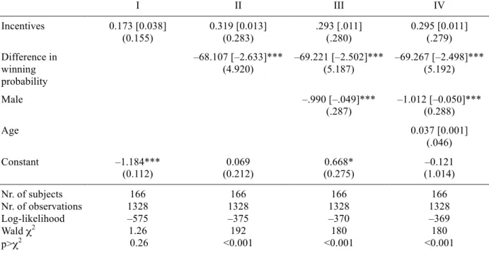
Table 1: Determinant of choice of the large urn in experiment 1 (random-effects Probit models)

I II III IV Incentives 0.173 [0.038] (0.155) 0.319 [0.013] (0.283) .293 [.011] (.280) 0.295 [0.011] (.279) Difference in winning probability –68.107 [–2.633]*** (4.920) –69.221 [–2.502]*** (5.187) –69.267 [–2.498]*** (5.192) Male –.990 [–.049]*** (.287) –1.012 [–0.050]*** (0.288) Age 0.037 [0.001] (.046) Constant –1.184*** (0.112) 0.069 (0.212) 0.668* (0.275) –0.121 (1.014) Nr. of subjects Nr. of observations Log-likelihood Wald χ2 p>χ2 166 1328 –575 1.26 0.26 166 1328 –375 192 <0.001 166 1328 –370 180 <0.001 166 1328 –369 180 <0.001

Note: Marginal effects in square brackets, standard errors in round brackets; * significant at 5% level, ** significant at 1% level, *** significant at 0.1% level, two-sided.

As can be seen from the results reported in Table 1, incentives do not have a significant effect. As one might expect, the difference in probability of winning between the two urns exerts a strong influence on choices. There is also a strong gender effect, while age exerts no significant effect—which is hardly surprising, given the low variability of age in the subject population.

2.3 Discussion

With 23% of choices of the large, inferior urn, when the latter offers a probability of winning of 9/100 against the 1/10 of the small urn, we do indeed find a ratio bias. However, this bias appears to be much weaker than its occurrences previously observed in the literature. Indeed, Denes-Raj and Epstein (1994) found between 61% and 54% of choices of the large inferior urn for the same probability, and Dale et al. (2007) found about 42% of choices of the large urn for the same probability difference. Incentives are not effective at further reducing the bias found. It thus seems that the weakening of the bias stems from the measures put into place to avoid experimenter

(13)

demand effects.

One potential criticism is however that incentives provided were too low to make the decisions seem important to the subjects. Although the nominal prize was high, the probability of extraction of any single choice in the ratio bias task was only 1/120. While no difference between random incentives and deterministic incentives has generally been found in the literature (Hey and Lee, 2005; Lee, 2008; Starmer and Sugden, 1991), the probability of extraction in this task was indeed extremely low, and certainly outside the range for which effects of random incentives have been tested. Also, the combination of random extraction of one subject, random extraction of one out of three tasks, and random extraction of one choice within that task may have created a feeling of irrelevance.

A second criticism that can be brought against the results presented above is that error was not explicitly controlled for. While it is true that choices for the inferior urn for the smallest probability difference of 1% are still hovering around 23%, it is not unthinkable that a large

proportion of these choices were due to noise and that the relevance of the ratio bias phenomenon is thus much lower than a first look at the data would suggest. Indeed, Dale et al. (2007) found error rates that are very similar to the occurrence of the bias in our experiment, even though they still found a significant ratio bias in excess of those errors. Admittedly, the employment of a 5% error rate against which to test the occurrence of the bias used above is utterly arbitrary and will be dealt with in experiment 2.

A number of other criticisms can be brought against the design. Indeed, one could argue that the sequential presentation of the choices in a fixed order induces some coherence effect by which subjects who have chosen the large urn when the two urns were probabilistically equivalent are more likely to stick with the choice of the large urn. Another potential criticism is that the bias persists due to the artificiality of the laboratory task. Indeed, context has sometimes been shown to improve rationality (Griggs, 1995), though the existing evidence on the ratio bias seems to rather

(14)

1 2

point in the direction of an accentuation of irrationality when context is added (Pinto, Martinez, and Abellán, 2006; Yamagishi, 1997). Since however no incentives were provided in previous

experiments, nothing can be said about their economic significance.

3. EXPERIMENT 2: CONTROLLING FOR ERROR AND UNIVERSAL INCENTIVES

Experiment 2 tries to obviate to the potential criticisms described above in several ways. First of all, we introduce deterministic incentives whereby every subject plays for real money. Second, we introduce some control choices in which the large urn is superior, which enables us to explicitly control for the error rate. Dale et al. (2007) control for error rates and still find a significant ratio bias. However, the incentives they provide are in the order of 5¢–10¢, which implies a negligible difference in expected value between the two urns. By making incentives more salient, we want to test whether the phenomenon is indeed stable. We thus use two stake levels, regular stakes which are already superior to the stakes found in previous experiments on the ratio bias, and a treatment in which stakes were increased by a factor of 10.

In addition, we try to minimize experimenter demand effects by reassuring subjects of their anonymity and by randomizing both the order in which choices appear as well as the position in which the options are presented within one choice (i.e. whether the small urn is located above or below the large one). Furthermore, we use both certainty equivalent (CE) and pricing tasks in addition to choices and we introduce context into some decision problems to test the robustness of the ratio bias to the nature of tasks. Last, we implement both a between-subject design and a within-subject design to investigate the potential policy relevance of the ratio bias phenomenon.

(15)

1

3.1 Experimental design: General remarks

Subjects. The experiment has been conducted at GATE (Groupe d’Analyse et de Théorie Economique), at the University of Lyon, France. 78 undergraduate students from the local

engineering and business schools were recruited using the ORSEE software developed by Greiner (2004). 64% of subjects were female, the average age was 22. Sessions were conducted in the computer laboratory in groups of 20 subjects. In one High-Stakes session only 19 subjects showed up. One more subject in the High-Stakes condition had to be sent away because of technical issues with the computer station. We thus ended up with 40 subjects in the Low-Stakes condition and 38 subjects in the High-Stakes condition.

Structure. Several tasks were used to explore the ratio bias phenomenon. In addition to choice tasks similar to the ones used in experiment one, we also used investment and insurance tasks, as well as a context-free task in which certainty equivalents were elicited. Also, we elicited values both within and between subject to test for policy relevance of the issues discussed. The three types of choices are discussed separately below. Subjects were reassured about their anonymity, and all instructions were provided on the computer screen (see Appendices). Finally, differently from Dale et al. (2007) and Denes-Raj and Epstein (1994), but similarly to our experiment 1, urns were not visually

displayed. This difference seems however not to be crucial, given that studies without visualization have also found a large ratio bias (Bonner and Newell, 2008; Pinto et al., 2006; Yamagishi, 1997). The experiment was conducted using the REGATE software (Zeiliger, 2000). Subjects were given a show-up fee of €5 ($7). Average earnings were €23.62 ($35) for an experiment that lasted less than 30 minutes.

(16)

1 4

3.2 Choice tasks

Task. The task consisted in repeated choices between lotteries. Subjects made 25 choices in total. The choice pairs were designed in such a way as to allow us to control for error, as well as to explore potential drivers of the ratio bias phenomenon. Both the order of the choice pairs and the location of the large versus small urn on the screen (above versus below) were randomized for each subject. Each choice pair involved a choice between one large urn and one small urn. 3 choice pairs provided the same probability for the large and small urn; 18 choice pairs provided a better

probability of winning in the small urn than in the large urn; and 4 choice pairs provided a worse probability of winning in the small urn than in the large urn to control for random errors. A list of the choice pairs used is provided in Appendix B, together with a screenshot of the choice setting subjects faced on the computer.

Incentives. Incentives were varied randomly within subject between a prize of €2, €7, and €12 ($3, $10, and $18) for half the subjects. The other half was assigned to the High-Stakes condition, in which the prize was varied randomly between €20, €70, and €120 ($30, $100, and $180). For one choice pair, the prize was kept fixed at €4 and €40 in the two conditions. This was done to insure comparability with the comparative investment task described below—since no interesting results emerged from this comparison, it will not be mentioned further. This randomly extracted prize as well as the descriptions of the two urns were displayed prominently on the screen for each decision. Every subject played one of the 25 choices for real money, with each choice having the same probability of being played for real. The random draw for this choice task (as well of the random draws for the following tasks) was operated at the very end of the session so that its outcome could not influence further choices.

(17)

1

Hypotheses. We hypothesize that the proportion of choices for the large urn when the latter provides the same probability as the small urn is significantly greater than 50%. Also, we hypothesize that the choice frequency of the large urn is significantly greater than the error rate (that is, the proportion of choices for the large urn when the latter provides probabilities of winning that are inferior to the ones provided by the small urn is significantly higher than the number of choices of the small urn providing inferior probabilities of winning). We also want to test whether varying incentives within subjects produces significant differences in behavior. Finally, we were interested if the ratio bias phenomenon may be reduced with very high stakes varied between subjects.

Results. General choice patterns are summarized in Figure 2 separately for the Low- and High-Stakes conditions. Overall, the large urn was chosen only 47% of the time when offering the same probability of winning as the small urn. We thus cannot reject the null hypothesis that in cases of equal probability the large urn will be chosen 50% of the time (p = 0.33, binomial test). When the large urn is inferior, it is chosen on average 7.19% of the time. The ratio bias in this experiment is thus much smaller than the one observed in experiment one. Looking now at the error rate, we see that the small urn is chosen on average 9.61% of the time when it is inferior. We can thus not reject the hypothesis that the frequency of choices consistent with a ratio bias explanation is the same as the error rate (t(77) = –0.47, p = 0.64).

(18)

1 6

Figure 2: Percentage of choices of the large urn by difference in the probability of winning

for the Low- and the High-Stakes conditions

We next look at the influence of within-subject stake variations, between-subject stake variations, and several other potential explanatory variables. We have estimated the determinants of the probability of choice of the large urn by means of four random-effects Probit models. The independent variables include the normalized prize that captures the within-subject variation of stakes, and a dummy variable indicating the High-Stakes condition. We also include a dummy variable (‘large urn superior’) indicating the choice pairs in which the large urn is superior, used to control for error, and another dulmmy variable (‘equal probability’) indicating that the two choices offered the same probability of winning. We also control for the probability difference between the two urns, calculated as the probability of winning with the small urn minus the probability of

winning with the large urn. In the last regression, we include demographic variables. Table 2 reports the results of these regressions.

(19)

1

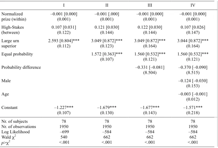
Table 2: Determinants of choice of the large urn in experiment 2 (random-effects Probit models)

I II III IV Normalized prize (within) –0.001 [0.000] (0.001) –0.001 [.000] (0.001) –0.001 [0.000] (0.001) –0.001 [0.000] (0.001) High-Stakes (between) 0.107 [0.031] (0.122) 0.121 [0.030] (0.144) 0.122 [0.030] (0.144) 0.107 [0.026] (0.147) Large urn superior 2.593 [0.804]*** (0.112) 3.049 [0.872]*** (0.123) 3.049 [0.872]*** (0.164) 3.044 [0.872]*** (0.164) Equal probability 1.572 [0.363]*** (0.107) 1.560 [0.532]*** (0.121) 1.560 [0.532]*** (0.121) Probability difference –0.331 [–0.081] (8.504) –0.370 [–0.090] (8.515) Male –0.124 [–0.030] (0.153) Age –0.003 [–0.001] (0.012) Constant –1.227*** (0.107) –1.679*** (0.130) –1.677*** (0.143) –1.571*** (0.218) Nr. of subjects Nr. of observations Log Likelihood Wald χ2 p>χ2 78 1950 –699 540 <.001 78 1950 –584 662 <.001 78 1950 –584 662 <.001 78 1950 –584 662 <.001

Note: Standard errors in round brackets, marginal effects in square brackets; * significant at 5% level, ** significant at

1% level, *** significant at 0.1% level, two-sided.

Table 2 shows that neither the within-subject variation in prizes (normalized across stakes conditions) nor the between-subject stake variation have any significant effect on decisions. As expected, when the large urn is superior subjects are significantly more likely to choose it than when it is inferior. In contrast, when the two urns provide an equal winning probability people are less likely to choose it than when it is inferior. The difference in the probability of winning exerts no further influence. Gender is no longer significant.

Discussion. At first sight, there seems to be a small ratio bias, even though it stays below 10% on average. Controlling however for error rates, these regressions show that these choices are entirely due to error or noise, inasmuch as there is no systematic preference pattern for the larger urn. This result remains stable across different stake levels, both within- and between-subject. The latter

(20)

1 8

finding can be explained by the fact that choices of the large urn are already substantially reduced in the Small-Stakes condition. Indeed, providing stakes of €7 ($10) on average to every participant combined with randomization and confidentiality of choices seems already to be sufficient to eliminate the bias. Given that choices of the inferior urn are already very low in the baseline condition, multiplying the stakes by a factor of 10 has no further effects.

Since some of the recent claims on the importance of the ratio bias phenomenon have been obtained through rating tasks rather then choices, we next examine comparative evaluations.

3.3 Comparative valuation tasks: Adding context

Employing comparative rating tasks rather than choice tasks generally adds context in addition to the different elicitation method used. Health economics issues generally studied however have the disadvantage of not easily allowing for the introduction of real incentives. We thus propose to use an investment task to add context whilst being able to implement the value elicitation in an incentive compatible way. In addition to the investment task, we also use an insurance task to test whether negative outcomes may be more prone to ratio bias than positive outcomes. While using losses has been found to produce less ratio bias than gains in choice tasks (Denes-Raj and Epstein, 1994; Kirkpatrick and Epstein, 1992), the risk rating tasks used in the health economics literature do generally involve losses and have found a very large ratio bias (Bonner and Newell, 2008; Pinto, Martinez, and Abellán, 2006; Yamagishi, 1997).

Tasks. In the investment task, subjects were presented with two investment projects, project A and project B. The two projects were displayed on the same screen, and choices had to be made between investing increasing amounts in each one of the investment projects and not investing (choice lists in Appendix C). Project A offered a probability of success of 7/100, and project B of 61/1000. In

(21)

1

the insurance task, subjects were offered to buy insurance against a low probability loss of their €5 ($7) show-up fee (see Appendix C). The risks in the insurance task were 59/1000 and 423/10000 respectively.

Incentives. Both tasks described above were played for real money. For the investment task, subjects were given an initial endowment of €0.60 (90¢) in the Low-Stakes condition, and €6 ($9) in the High-Stakes condition. The prize to be won in the two investment tasks was of €4 ($6) in the Low-Stakes condition and €40 ($60) in the High-Stakes condition. In the insurance task, the amount to be lost was not varied and stayed fixed at the show-up fee of €5 ($7). For either task, at the end of the session one of the two investment projects or insurance scenarios would first be randomly selected for real play. Then one of the decisions would be selected and played for real. In the investment task, if a subject had decided not to invest for the selected line, she could keep her endowment and the game was over. If she had selected to invest, the investment amount was

subtracted from the endowment and the prospect was played out. An analogous procedure was used for the insurance task.

Hypotheses. The two investment projects and insurance scenarios are characterized by different probabilities, as well as being represented with small versus large ratios. We thus hypothesize that the difference that subjects are willing to pay over the expected value of the investment (or the expected loss in the insurance case) will be larger for the large ratio than for the small ratio.

Results. Five subjects in the investment task and two subjects in the insurance task were excluded from the analysis because they switched multiple times between the certain amount and the

(22)

2 0

willingness-to-pay for these subjects. Since probabilities differ in the two investment opportunities, a test for equality of amount invested is not adequate. We thus calculate the difference between the highest amount subjects are willing to invest in each project and the expected value of the

investment, and test for equality of this premium. The mean values of the premia are reported in Table 3 separately for low and high stakes. No High-Stakes condition existed in the comparative insurance task; all subjects played for the show-up fee of €5 ($7). Table 3 also reports the mean amount subjects are willing to pay for the insurance in excess of the expected value of the loss.

Table 3: Mean amounts in excess of expected values (premia) that subjects are willing to pay, in €

Project/Scenario A Project/Scenario B Investment – Low-Stakes* 1.46 (0.21) 1.39 (0.25) Investment – High-Stakes 0.89 (0.31) 0.48 (0.34) Insurance 0.42 (0.04) 0.47 (0.04)

Note: * Values are normalized to high stakes amounts through multiplication by 10; standard deviations in brackets.

While the excess premia appear to be much lower in the High-Stakes than in the Low-Stakes condition, we cannot reject the null hypothesis that the two premia are the same in the Low-Stakes condition (t(39) = 0.58, p = 0.56). For the High-Stakes condition, we find a marginally significant difference between the two premia (t(32) = –1.99, p = 0.06). Notice however that this effect goes in the opposite direction of the one predicted by the ratio bias hypothesis. In the insurance task, testing the null hypothesis that the premium paid over the expected value of the loss is equal in the two scenarios, we reject that hypothesis in favor of the one that the premium is higher for the larger ratio (t(78) = 2.08, p = 0.04). This would lead us to conclude that ratio bias does indeed occur. Before we jump to such a conclusion, it is however instructive to take a closer look at the data. For scenario A, 39 subjects out of 76 (51.32%) never switch between the sure amount and the prospect, with an

(23)

2

overwhelming majority of those who never switch (33/39) willing to buy insurance at any amount it was offered at (and the remaining 6 never willing to buy insurance). A similar finding holds for scenario B, in which 41 out of 76 subjects (53.95%) never switch. Again, an overwhelming majority of subjects who never switch (33/41) are willing to take out insurance at any cost it was offered at. The results of the previously reported t-test thus seems to be due to a ceiling effect in the prices at which insurance was offered. Indeed, we cannot reject the hypothesis that the number of subjects who never switch is the same for scenarios A and B (t(73) = –1.0, p = 0.32). Given that the expected value is lower for scenario B, these subjects are likely to drive the results. Carrying out the same test as above only for subjects that do switch and are thus not at the margin, we accept the null hypothesis that no ratio bias exists (t(29) = 0.48, p = 0.64).

Discussion. We find no ratio bias when we add context to the decisions, and when decisions consist in comparative pricing tasks instead of straight choice tasks. A ratio bias is found neither for gains nor for losses. However, in the insurance task we lose some power due to the ceiling effects

described above. Indeed, due to the choice list employed for the elicitation of the willingness-to-pay for insurance, the maximum willingness-to-pay that could be stated was about 3-4 times the

expected value of the loss, depending on the scenario. Quite a few subjects were willing to pay more than that amount to buy insurance. This finding is consistent with findings in the literature on strong loss aversion (Kahneman and Tversky, 1979; Köbberling and Wakker, 2005; Schmidt and Zank, 2005) and the excessive uptake of insurance (Hogarth and Kunreuther, 1989).

In addition, we find the typical pattern of risk seeking for small probability gains. Subjects are on average willing to invest an amount in excess of the expected value of the prospect in the investment task. This finding is consistent with the evidence presented in the literature on probability weighting, and in particular with overweighting of small probabilities (Abdellaoui, 2000; Bleichrodt and Pinto, 2000; Tversky and Kahneman, 1992; Wu and Gonzalez, 1996). Also,

(24)

2 2

this risk seeking behavior seems to be reduced in the High-Stakes condition, which is also

consistent with previous findings in the literature (Battalio, Kagel, and Jiranyakul, 1990; Holt and Laury, 2002). Since this finding has however wider implications, it is described in a separate paper in order not unduly complicate the exposition (Lefebvre, Vieider, and Villeval, 2009).

At this point, there is still one objection that can be raised to our analysis. Indeed, while all existing studies on the ratio bias employ either choice or rating tasks - and hence a strictly

comparative setting - the potential policy relevance of the phenomenon may derive from the fact that probabilities represented as large ratios are overestimated more than equivalent small-ratio probabilities when considered in isolation. We thus next examine results on between-subject tests of the ratio bias phenomenon.

3.4 Between-subject data: Policy relevance

Recent results on the ratio bias phenomenon especially in the medical domain have been used to draw conclusions on the importance of the phenomenon for risk communication and policy issues. While we have not been able to replicate the ratio bias phenomenon in the experiments presented above, for risk communication and policy issues it would arguably be more important to know whether such a bias in risk evaluation might exist when only one way of communicating the risk is used at a time. Indeed, in reality risk is generally communicated just in one way, and it seems thus crucial to know whether a ratio bias is observed between subjects before proceeding to policy recommendations. To our best knowledge, this issue has never been addressed before. We thus introduced some between-subject rating tasks at the outset of the experiment before any

comparative tasks were introduced in order to test for this hypothesis. We also added context in some of them, to see if such context may make a difference. Details are reported below.

(25)

2

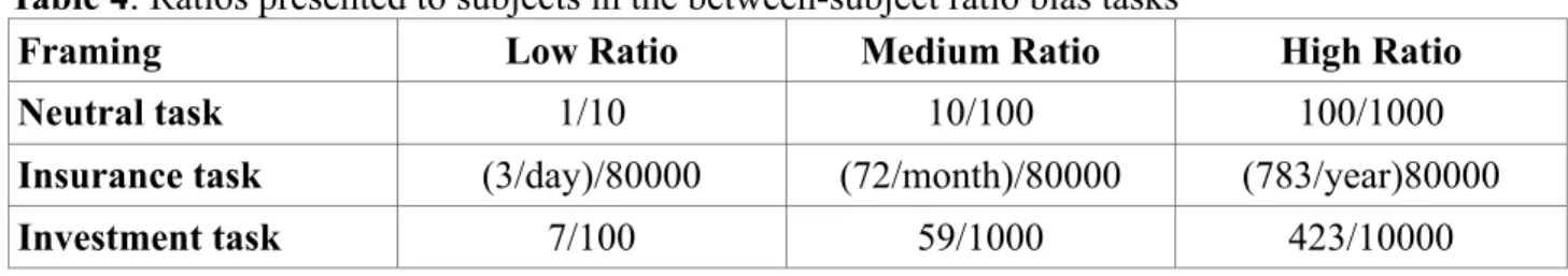
Tasks. Three different tasks were introduced in a between-subject design in order to test for a between-subject ratio bias phenomenon. Each subject saw one of three ratios in the description of the problem. We used three ratios instead of two to create more variance. The assignment of the ratio was randomly and independently determined for each subject and for each one of the three tasks (ratios are reported in Table 4). Task one (the neutral task) consisted in repeated choices between an increasing certain amount of money and a prospect offering the opportunity to win a prize. The second task (the insurance task) offered the opportunity to buy insurance against the possibility of losing the prize won in the neutral task. It was to be played out for real money at the end of the session only in case a subject had won the prize in task one. In task three (the investment task), subjects were asked to choose for subsequent amounts whether they would rather keep the amount or invest it.

Table 4: Ratios presented to subjects in the between-subject ratio bias tasks

Framing Low Ratio Medium Ratio High Ratio

Neutral task 1/10 10/100 100/1000

Insurance task (3/day)/80000 (72/month)/80000 (783/year)80000

Investment task 7/100 59/1000 423/10000

Incentives. The neutral task was to be played out for real money, offering a prize of €10 ($15) in the Low-Stakes condition and €100 ($150) in the High-Stakes condition. Subjects were asked to choose between a sure amount (certainty equivalent,) and playing the prospect for increasing certain

amounts (see Appendix D). One line would be selected for real play at the end of the session, and the subject would either be paid the sure amount or play the prospect according to her choice for that line. In the investment tasks, subjects were initially endowed with €0.60 (90¢) in the Low-Stakes condition and €6 ($9) in the High-Low-Stakes condition. They were asked whether they were willing to invest increasing amounts of their endowment, with a potential return of €4 ($6) in the

(26)

2 4

Low-Stakes condition and €40 ($60) in the High-Stakes condition. One choice was then selected through a procedure analogous to the one used in the neutral task, except that if they had chosen to invest, the corresponding amount was now subtracted from their endowment before playing the prospect. The insurance task was to be played out conditional on a subject having won the prize in the neutral task only. A procedure analogous to the one in the investment task was then used to determine payoffs (all choice lists can be found in Appendix D).

Hypotheses. We hypothesize that subjects have a higher certainty equivalent the larger the urn in the neutral task, since probabilities are equal in those tasks. For the insurance task, we hypothesize that subjects are ready to pay a higher amount in excess of the expected value of the loss (probabilities are now different) as we pass from representations per day to month and year. Analogously, we hypothesize that for the investment task subjects are willing to invest more in excess of the expected value as we move to larger ratios.

Results. In the neutral task, six subjects were dropped because they switched multiple times. All of these subjects were in the High-Stakes condition. We dropped for the same reason two subjects in the insurance task and six subjects in the investment task. Table 5 displays the mean valuation of the subjects in each task and for each ratio.

(27)

2

Table 5. Mean valuations in the between-subject tasks

Note: Standard deviations are in brackets.

Running an Anova on the certainty equivalents for the three different ratios in the neutral task, no significant difference is found (F(2,69) = 0.63, p = 0.54). The null hypothesis of equal certainty equivalents for different ratios can thus not be rejected. No significant difference is found if the same Anova is run separately for the Low-and the High-Stakes conditions, although we again find a reduction in risk seeking for high stakes.

In the insurance task, since probabilities of losing are now different we calculate the excess premium that subjects are willing to pay over the expected value of the loss for each ratio, and run an Anova on these derived values. In the Low-Stakes condition, there is a marginally significant effect indicating a ratio bias (F(2,37) = 2.83, p = 0.07). This effect is however not significant in the High-Stakes condition (F(2,33) = 2.27, p = 0.12). Also, a closer look at the data reveals that the result is mostly driven by a substantial amount of subjects (37/76 or 48.68%) who never switch, and who are equally distributed across the different ratios. All but one of these subjects choose to insure at any price the insurance is offered at. Once those subjects are eliminated, no significant

differences persists between the excess premia paid for the different urns.

Value in € Low Ratio Medium Ratio High Ratio

Neutral task - Certainty equivalent

(normalized to high stakes)

14.50 (6.29) n=29 12.65 (5.89) n=20 12.94 (6.77) n=23 Insurance premium 13.42 (7.13) n=29 13.99 (7.04) n=21 14.50 (6.05) n=26 Insurance premium minus

expected value 2.47 (7.13) 5.35 (7.04) 6.67 (6.04) Maximum investment 3.92 (1.76) n=25 3.59 (1.77) n=31 4.32 (1.86) n=16 Maximum investment minus

expected value 1.12 (1.76) 1.23 (1.77) 2.62 (1.86)

(28)

2 6

In the investment task, since probabilities of success are again different for the different ratios, we calculated the excess investment premium over expected value that subjects were willing to pay for each ratio. Running an Anova on this index for the Low-Stakes condition, we find a significant difference (F(2,35) = 3.28, p = 0.05), indicating the presence of ratio bias. Running the same Anova for the High-Stakes condition, the difference is no longer significant (F(2, 31) = 0.93, p = 0.41).

Discussion. In general, we detect no ratio bias in the three between-subject tasks described in this section. Although at first glance there seems to be a marginally significant effect in the insurance setting, closer inspection of the data reveals that this finding is driven entirely by a ceiling effect on amounts that can be selected for insurance. This ceiling effect seems to derive from extreme loss aversion that is summed to the overweighting of small probabilities as discussed for the

comparative insurance task above. Also, while there is some evidence for the ratio bias

phenomenon in the investment task for small stakes, this effect is no longer present for large stakes. We thus conclude that the alleged policy relevance of the ratio bias phenomenon is doubtful at best.

4. CONCLUSION

From the experiments conducted, it results clearly that the ratio bias that has been observed in choice tasks in the literature results from a combination of the failure to control for error, the presence of experimenter demand effects, and the absence of salient and dominant incentives. Indeed, by reducing the possibility of demand effects in experiment 1 we observe a frequency of ratio bias that is greatly reduced as compared to previous studies. Introducing significant incentives for everybody, further reducing the possibility of demand effects, and controlling for errors causes the ratio bias to disappear in experiment 2. This finding is robust even when context is added to the

(29)

2

decision problem, and for gain as well as loss formulations. Finally, no ratio bias is found

systematically in between-subject tests either, with only some evidence in the investment task that does not resist an increase in monetary stakes. These results cast serious doubts on claims about the policy relevance of the ratio bias phenomenon.

(30)

2 8

Appendix A. Choices between lotteries to detect ratio bias – Experiment 1

Problem 1

Bag A contains 10 poker chips, 1 red chip and 9 green chips. Bag B contains 100 poker chips, 10 red chips and 90 green chips. You can win €80 by extracting a red chip from one of the two bags. Which bag do you choose?

Bag A (1 red chip and 9 green chips) Bag B (10 red chips and 90 green chips)

Problem 2

Problem 3

Problem 4

Problem 5

Problem 6

Problem 7

Problem 8

Bag A contains 10 poker chips, 1 red chip and 9 black chips. Bag B contains 100 poker chips, 3 red chips and 97 green chips. You can win €80 by extracting a red chip from one of the two bags. Which bag do you choose?

(31)

2

Appendix B – Screenshots of the choice tasks – Experiment 2

Decision Pair Low Ratio (small urn) High (large urn)

Pair 1 1/10 10/100 Pair 2 1/10 9/100 Pair 3 1/10 8/100 Pair 4 10/100 100/1000 Pair 5 10/100 93/1000 Pair 6 10/100 87/1000 Pair 7 1/100 10/1000 Pair 8 1/100 7/1000 Pair 9 1/100 5/1000 Pair 10 1/1000 92/10000 Pair 11 6/1000 57/10000 Pair 12 23/1000 211/10000 Pair 13 33/10000 297/100000 Pair 14 27/10000 237/100000 Pair 15 03/74 27/740 Pair 16 1/56 9/560 Pair 17 1/257 10/2586 Pair 18 1/10 91/1000 Pair 19 1/10 793/10000 Pair 20 5/100 432/10000 Pair 21 1/10 11/100 Pair 22 02/74 24/740 Pair 23 7/1000 75/10000 Pair 24 11/100 99/1000 Pair 25 7/100 61/1000

(32)

3 0

(33)

3

(34)

3 2

(35)

3

(36)

3 4

(37)

3

REFERENCES

Abdellaoui, Mohammed (2000). Parameter-Free Elicitation of Utility and Probability Weighting Functions. Management Science 46(1), 1497-1512.

Abdellaoui, Mohammed, Aurélien Baillon, and Peter P. Wakker (2007). Combining Bayesian Beliefs and Willingness to Bet to Analyze Attitudes towards Uncertainty. Econometric Institute, Erasmus University, Rotterdam, the Netherlands.

Battalio, Raymond C., John H. Kagel, and Komain Jiranyakul (1990). Testing Between Alternative Models of Choice under Uncertainty. Journal of Risk and Uncertainty 3, 25–50.

Bleichrodt, Han, and José Luis Pinto (2000). A Parameter-Free Elicitation of the Probability Weighting Function in Medical Decision Analysis. Management Science 46(11), 1485-1496. Bonner, Carissa, and Ben R. Newell (2008). How to Make a Risk Seem Riskier: The Ratio Bias

versus Construal Level Theory. Judgment and Decision Making 3(5), 411-416. Camerer, Colin F., and Robin M. Hogarth (1999). The Effects of Financial Incentives in

Experiments: A Review and Capital-Labor-Production Framework. Journal of Risk and Uncertainty, 19(1), 7-42.

Camerer, Colin F., and Martin Weber (1992). Recent Developments in Modeling Preferences: Uncertainty and Ambiguity. Journal of Risk and Uncertainty 5, 325-370.

Chow, Clare Chua, and Rakesh K. Sarin (2001). Comparative Ignorance and the Ellsberg Paradox. Journal of Risk and Uncertainty 22, 129-139.

Denes-Raj, Veronika, and Seymour Epstein (1994). Conflict Between Intuitive and Rational Processing: When People Behave Against Thir Better Judgment. Journal of Personality and Social Psychology 66(5), 819-829.

Denes-Raj, Veronika, Seymour Epstein, and Jonathan Cole (1995). The Generality of the Ratio-Bias Phenomenon. Personality and Social Psychology Bulletin 21, 1083-1092.

Einhorn, Hillel J., and Robin M. Hogarth (1986). Ambiguity and uncertainty in probabilistic inference. Psychological Review 92(4), 433-461.

Eisenberger, Roselies, and Martin Weber (1995). Willingness-to-Pay and Willingness-to-Accept for Risky and Ambiguous Lotteries. Journal of Risk and Uncertainty 10, 223-233.

Frisch, Deborah, and Jonathan Baron (1988). Ambiguity and Rationality. Journal of Behavioral Decision Making 1, 149-157.

Greenwald, Anthony G. (1978). Within-Subject Designs: To Use or Not to Use? Psychological Bulletin, 314–320.

Greiner, Ben (2004). An Online Recruitment System for Economic Experiments. In: K. Kremer, V. Macho (Eds.): Forschung und wissenschaftliches Rechnen 2003. GWDG Bericht 63,

Göttingen: Ges. fü r Wiss. Datenverarbeitung, 79-93.

Griggs, Richard A. (1995). The Effects of Rule Clarification, Decision Justification, and Selection Instruction on Wason’s Abstract Selection Task. In S.E. Newstead and J. St. B.T. Evans (eds.) “Perspectives on Thinking and Reasoning”, Lawrence Erlbaum Associates: Hove.

Harrison, Glenn W., Morten I. Lau, and Melonie B. Williams (2002), “Estimating Individual

Discount Rates in Denmark: A Field Experiment,” American Economic Review 92, 1606−1617. Hertwig, Ralph, and Andreas Ortmann (2001). Experimental Practices in Economics: A

(38)

3 6

Methodological Challenge for Psychologists? Behavioral and Brain Sciences 24, 383-451. Hey, John D. and Jinkwon Lee (2005). Do Subjects Separate (or Are They Sophisticated)?

Experimental Economics 8, 233−265.

Hogarth, Robin M., and Howard Kunreuther (1989). Risk, Ambiguity and Insurance. Journal of Risk and Uncertainty 2, 5-35.

Holt, Charles A. (1986). Preference Reversals and the Independence Axiom. American Economic Review 76(3), 508-515.

Holt, Charles A., and Susan K. Laury (2002). Risk Aversion and Incentive Effects. American Economic Review, 1644-1655.

Kahneman, Daniel, Jack L. Knetsch, and Richard H. Thaler (1991). Anomalies: The Endowment Effect, Loss Aversion, and Status Quo Bias. Journal of Economic Perspectives 5(1), 193-206. Kahneman, Daniel, and Amos Tversky (1979). Prospect Theory: An Analysis of Decision under

Risk. Econometrica 47(2), 263-291.

Kirkpatrick, Lee A., and Seymour Epstein (1992). Cognitive-Experiential Self-Theory and Subjective Probability: Further Evidence for Two Conceptual Systems. Journal of Personality and Social Psychology 63(4), 534-544.

Köbberling, Veronika, and Peter P. Wakker (2005). An Index of Loss Aversion. Journal of Economic Theory 122, 119-131.

Kocher, Martin. G., and Stefan T. Trautmann (2008). Selection in Markets for Risky and Ambiguous Prospects. Working Paper.

Lee, Jinkwon (2008). The Effect of the Background Risk in a Simple Chance Improving Decision Model. Journal of Risk and Uncertainty 36, 19-41.

Lefebvre, Mathieu, Ferdinand M. Vieider, and Marie Claire Villeval (2009). A Note on the Effect of Between Subject Stake Variations on Risk Attitude. Working Paper, Laboratoire GATE, Université de Lyon.

Lichtenstein, Sarah, and Paul Slovic (1971). Reversals of Preference Between Bids and Choices in Gambling Decisions. Journal of Experimental Psychology 89(1), 46-55.

Miller, Dale T., William Turnbull, and Cathy McFarland (1989). When a Coincidence is Suspicious: The Role of Mental Simulation. Journal of Personality and Social Psychology 57(4), 581-589. Minor, Marshall W. (1970). Experimenter-Expectancy Effect as a Function of Evaluation

Apprehension. Journal of Personality and Social Psychology 15(4), 326-332.

Myagkov, Mikhail G. and Charles R. Plott (1997). Exchange Economies and Loss Exposure: Experiments Exploring Prospect Theory and Competitive Equilibria in Market Environments. American Economic Review 87, 801−828.

Pacini, Rosemary, and Seymour Epstein (1999). The Relation of Rational and Experiential Information Processing Styles to Personality, Basic Beliefs, and the Ratio-Bias Phenomenon. Journal of Personality and Social Psychology 76(6), 972-987.

Pinto-Prades, José-Luis, Jorge-Eduardo Martinez-Perez, and José-Maria Abellán-Perpiñán (2006). The Influence of the Ratio Bias Phenomenon on the Elicitation of Health States Utilities. Judgment and Decision Making 1(2), 118-133.

Reyna, Valerie F., and Charles J. Brainerd (2008). Numeracy, Ratio Bias, and Denominator Neglect in Judgments of Risk and Probability. Learning and Individual Differences 18, 89-107.

(39)

3

Roca, Mercé, Robin M. Hogarth, and A. John Maule (2006). Ambiguity Seeking as a Result of the Status Quo Bias. Journal of Risk and Uncertainty 32(3), 175-194.

Sawyer, Alan G. (1975). Demand Artifacts in Laboratory Experiments in Consumer Research. Journal of Consumer Research 1(4), 20-30.

Schmidt, Ulrich, Starmer, Chris, and Sugden, Robert (2008). Explaining Preference Reversal with Third-Generation Prospect Theory. Journal of Risk and Uncertainty 33(6), 203-223.

Schmidt, Ulrich, and Horst Zank (2005). What is Loss Aversion? Journal of Risk and Uncertainty 30(2), 157-167.

Slovic, Paul (2000). The Perception of Risk. Erthscan Publications Ltd, London and Sterling, VA. Starmer, Chris, and Robert Sugden (1991). Does the Random-Lottery Incentive System Elicit True

Preferences? An Experimental Investigation. American Economic Review 81, 971−978. Trautmann, Stefan T., Ferdinand M. Vieider, and Peter P. Wakker (2008). Causes of Ambiguity

Aversion: Known Versus Unknown Preferences. Journal of Risk and Uncertainly 36, 225-243. Trope, Yaacov, and Nera Liberman (2003). Temporal Construal. Psychological Review 110,

403-421.

Tversky, Amos, and Daniel Kahneman (1992). Advances in Prospect Theory: Cumulative Representation of Uncertainty. Journal of Risk and Uncertainty 5, 297-323.

Tversky, Amos, and Richard H. Thaler (1990). Preference Reversals. Journal of Economic Perspectives 4(2), 201-211.

Vieider, Ferdinand M. (2009). Separating Real Incentives and Accountability. Tinbergen Discussion Paper.

Wu, George, and Richard Gonzalez (1996). Curvature of the Probability Weighting Function. Management Science 42(12), 1676-1690.

Yamagishi, K. (1997). When a 12.86% mortality is more dangerous than 24.14%: Implications for Risk Communication. Applied Cognitive Psychology 11, 495-506.

Zeiliger, R. (2000). A Presentation of Regate, Internet Based Software for Experimental Economics, http://www.gate.cnrs.fr/~zeiliger/regate/RegateIntro.ppt, GATE. Lyon: GATE.