RESEARCH OUTPUTS / RÉSULTATS DE RECHERCHE
Author(s) - Auteur(s) :
Publication date - Date de publication :
Permanent link - Permalien :
Rights / License - Licence de droit d’auteur :
Institutional Repository - Research Portal
Dépôt Institutionnel - Portail de la Recherche
researchportal.unamur.be
University of Namur
Inequality and Demand-Driven Innovation
Kiedaisch, Christian; Dorn, Sabrina
Publication date:
2017
Link to publication
Citation for pulished version (HARVARD):
Kiedaisch, C & Dorn, S 2017 'Inequality and Demand-Driven Innovation: Evidence from International Patent Applications'.
General rights
Copyright and moral rights for the publications made accessible in the public portal are retained by the authors and/or other copyright owners and it is a condition of accessing publications that users recognise and abide by the legal requirements associated with these rights. • Users may download and print one copy of any publication from the public portal for the purpose of private study or research. • You may not further distribute the material or use it for any profit-making activity or commercial gain
• You may freely distribute the URL identifying the publication in the public portal ?
Take down policy
If you believe that this document breaches copyright please contact us providing details, and we will remove access to the work immediately and investigate your claim.
Inequality and Demand-Driven Innovation: Evidence
from International Patent Applications
[HIGHLY PRELIMINARY; PLEASE ONLY CITE WITH AUTHOR CONSENT]
You can download the most current version here.
Sabrina Dorn
∗Christian Kiedaisch
†March 20, 2017
Abstract
This paper studies how the distribution of income across consumers affects inno-vation by affecting the demand for new goods. Within a model with non-homothetic preferences, we show that inequality is more likely to be harmful for innovation when innovations become more incremental, but that it is more likely to be beneficial when the size of the population is increased. The model is extended to a multi-country setting in which it is shown that inequality affects the number of patent flows (ap-plications of patents that are already granted elsewhere) towards a country in the same way as it affects innovation. In an empirical analysis based on a large panel data set from PATSTAT, we find that inequality is more likely to increase and less likely to decrease international patent flows towards a country the larger the size of the population and the lower GDP of the country is. These results are in line with the model predictions and robust to the inclusion of many control variables.
∗me@sabrinadorn.com
†University of Zürich, christian.kiedaisch@econ.uzh.ch, I gratefully acknowledge financial support by
1 Introduction
This paper analyzes, both from a theoretical and empirical perspective, how the distri-bution of income across consumers affects innovation by affecting the demand for new goods. Innovation is the main driving force of long run growth and most governments are heavily involved in redistributing income in order to reduce the level of inequality. With income inequality on the rise in many developed countries (see for example Piketty, 2014), it is therefore important to understand how inequality and innovation are related. The motivation for this paper is that rich and poor households differ with respect to their consumption pattern and that rich households consume a larger variety of goods than poorer ones. This is for example shown in empirical studies conducted by Jackson (1984) and Falkinger and Zweimüller (1996). Using data from the US consumer expenditure survey, Kiedaisch (2016) shows that there is also a strong positive association between a more narrowly defined variety of “innovative” goods purchased by a household and household expenditures. When a new innovative good is more likely to be purchased by a rich household, the demand for it and the incentives to invent it therefore depend on the distribution of income.
In order to better understand the effect of inequality on innovation, we analyze a product variety model based on Föllmi and Zweimüller (2016) in which households either consume or do not consume a particular good, and in which rich households consume a larger variety of goods than poorer households. There are fixed costs of innovating and innovations lead to cost reductions that transform competitively supplied non-innovative into monopolistically supplied innovative goods. Households differ with respect to income and there is free entry into R&D. Within this setting, the incentives to innovate depend on the number of households that purchase an innovative good and also on their will-ingness’ to pay for the good. In equilibrium, poor households spend all their income on innovative mass consumption goods while rich households also purchase some luxurious non-innovative (service) goods (in Appendix A2, an extension is analyzed in which all households first purchase some non-innovative basic need goods like food before they start purchasing innovative goods and non-innovative luxuries. As long as most households are rich enough to purchase all basic need goods, the results remain the same).
The prices of innovative goods are inversely related to the number of households that purchase them in equilibrium. This implies that progressive transfers among poor households who spend all their income on innovative goods shift demand towards sectors with lower markups and thereby reduce the incentives to innovate and the number of innovations that are carried out. An reduction in inequality can therefore stiffle innovation through such price effects. When, however, income is redistributed from a rich household
who spends additional income on non-innovative luxuries to a poorer “mass consumer”, this increases the demand for innovative goods and the incentives to innovate.
Whether or not a progressive transfer between two randomly drawn households in-creases or dein-creases innovation depends on the endogenous fraction of households that spend all their income on innovative goods. This fraction increases when the size of the population increases (for a given total income), when innovations lead to larger cost re-ductions, and when total income decreases. The reasons for this are the following: due to the presence of substitutable non-innovative goods, innovators are restricted in their price setting power and can maximally charge a limit price. When the size of the population increases, an innovator selling at the limit price can break even by selling one unit of the innovative good to a smaller fraction of the population. When cost reductions are larger, the limit price increases and innovators can also break even by selling to a smaller fraction of the population. In both cases, the fraction of households that only consume innovative goods in equilibrium increases. When total income increases, overall more innovations are carried out and the marginal innovation is of lower value. This implies a lower limit price, forcing innovators to sell to a larger fraction of the population in order to break even. Taken together, these effects imply that a progressive (inequality-reducing) trans-fer between two randomly drawn households is less likely to encourage or more likely to discourage innovation the larger the size of the population is, the larger the size of the cost reductions of innovations are, and the lower total income is.
The model is extended to a multi-country setting with two types of fixed costs: Fixed costs of invention (that are borne only once), and country-specific fixed costs of (subse-quent) patenting or technology adoption. In this setting, inventors only pay the fixed costs of patenting or adoption when there is sufficient demand for an innovative good in a particular country (it is assumed that there is no parallel trade). In equilibrium, some countries endogenously emerge as “frontier” countries in which R&D is undertaken and others are “follower” countries in which only a fraction of the global stock of inventions get patented. When an innovation undertaken and patented in one country also gets subsequent patent protection in another country, a patent flow occurs between the two countries. The model predicts that inequality in a follower country is more likely to be good and less likely to be bad for the number of international patent flows towards this country the larger the size of the population, the larger the cost saving of the innovation, and the lower total income in this country is.
The qualitative (interaction) effects that inequality has on international patent flows towards a country are therefore the same as those that inequality has on innovation in the closed economy model. By empirically analyzing how inequality affects international patent flows we therefore hope to be able to infer how inequality affects innovation, at
least in a qualitative way.
From an empirical perspective, studying patent flows has the following advantages: while the incentives to innovate might be driven by the demand coming from several countries and not only the country of invention, a patent flow towards a single country usually only occurs if the profitability in this country is sufficiently large. There is there-fore a clearer definition of the relevant market. Moreover, we can study the variation in patent flows originating from the same set of technologies and do not need to compare heterogeneous innovations across countries. Furthermore, we believe that it is unlikely that a patent flow towards a country affects the level of inequality there (reverse causal-ity) as technologies might diffuse towards countries independently of whether they are (subsequently) patented there (see Appendix A3).
Based on raw-data from the PATSTAT data-base on patents of invention in the man-ufacturing sector within 1980-2013, we study the behavior of international patent-flows from a country of origin (frontier-country) to a different country (adopting-country) with respect to the implications of the claimed theoretical channel.
Using a rich set of control variables, and considering five different measures of in-equality (Gini coefficients pre- and post-taxes as well as top income shares) yielding to estimation samples of approximately 1,8 - 2,9 million observations, we find a strong sta-tistical pattern supporting the theoretical predictions. This is confirmed by four different estimators of the conditional expectation of patent-flows parametrized by an exponential mean model.
For a quantitative assessment of our estimation results, using a sample of 67 countries from 1980-2013, we may predict the incidence of a positive marginal effect of an increase in inequality for all empirically observed combinations of population and GDP over these countries as destinations and all points in time. We estimate the probabilities that an increase in inequality increases patent flows to be roughly 0.57 when inequality is measured in terms of Gini post-tax, 0.53 when it is measured in terms of Gini pre-tax, and 0.26, 0.23, and 0.11 when it is measured in terms of the top-10%, top-5%, and top-1% income share.
In an extension of the model, we find that strengthening patent protection makes it more likely that inequality increases (and less likely that it decreases) innovation. Measuring the strength of patent protection by the Ginarte-Park index, we indeed find this predicted positive interaction between patent protection and the effect of inequality on patent flows in our empirical analysis.
2 Related Literature (to be added)
The theoretical model builds on the analysis of Föllmi and Zweimüller (2016) who analyze the effect of inequality on growth in an endogenous growth model. The present model is static (i.e. there are only two periods), but, unlike Föllmi and Zweimüller (2016) considers the more general case where the size of the population can vary and where the value of the marginal innovation can depend on the number of innovations that have already been carried out. While Föllmi and Zweimüller merely show that inequality can be either beneficial or harmful for growth (depending on whether price or market size effects dominate), the present model shows that inequality is more likely good or less likely bad for innovation the larger the size of the population and the lower total income is. Moreover, we extend the model to an international setup in order to derive empirically testable implications, while Föllmi and Zweimüller (2016) only consider the case of a closed economy and do not undertake any empirical analysis.
3 Model
In this section we develop the theoretical model.
3.1 Preferences
All households have the same utility function given by
U = f (C) + D (1)
where C = RN
j=0cjdj denotes the variety of innovative goods and D = R1
n=0cndn the variety of non-innovative goods consumed. Goods are indivisible and households are assumed to be satiated with a particular good after consuming one unit of it. Therefore, households either consume one or zero units of any good (i.e. cj 2 {0; 1} and cn 2 {0; 1}). While there is an infinite variety of producible non-innovative goods1, only the endogenous measure N of innovative goods can be produced. It is assumed that f(C) is a continuous function satisfying @f (C) @C > 0, @2f (C) @C2 < 0, @f (C) @C C=0 = 1 and limC!1 @f (C) @C > c ⌦, where 0 < c
⌦ < 1 (the latter is an assumption on cost parameters which is explained further below). These assumptions imply that the utility derived from consuming an additional innovative good lies (weakly) below that of consuming an additional non-innovative good (which is constant) and that the former falls in the measure C of innovative goods that
1The analysis would be the same if there was instead only one divisible non-innovative good the
a household consumes2. The more innovative goods a household consumes the less it therefore values each single one of them relative to a non-innovative good. The analysis is, however, also carried out for the case in which the marginal utility from consuming innovative goods is constant, i.e. in which @2f (C)
@C2 = 0 and
@f (C)
@C = 1 holds for all values of C).
3.2 Endowments, technology, and market structure
Labor is the only production factor. The total labor endowment in terms of efficiency units is given by Y and the size of the population by L. Households are assumed to differ with respect to their labor productivities and a household of type ✓ is endowed with y(✓) = ✓YL efficiency units of labor. The type ✓ therefore indicates the labor endowment of the household divided by the average labor endowment in the economy (both measured in efficiency units). The variable ✓ is distributed with density g(✓) and cdf G(✓) in the interval between ✓ < 1 and ¯✓ > 1. As ✓ = y(✓)L
Y and Y = L R✓¯
✓ y(✓)g(✓)d✓, the condition R✓¯
✓ ✓g(✓)d✓ = 1 must hold.
For a given distribution G(✓) an increase in Y implies that all labor endowments y(✓) increase proportionally (i.e. an increasing scale transformation), while an increase in the size of the population L implies that all labor endowments are reduced proportionally (i.e. a decreasing scale transformation).
In order to produce one unit of a non-innovative good, ⌦ units of labor are required, while only c < ⌦ units are required in order to produce one unit of an innovative good. While the technology to produce non-innovative goods is in the public domain, innovative (low-cost) goods first need to be invented: The fixed costs F in terms of labor need to be paid in order to invent one innovative good j.
This set-up might be interpreted in the following way: Innovations transform non-innovative goods (e.g. traditional manufacturing goods or personal services) into inno-vative goods (e.g. modern manufacturing goods) that can be supplied at lower marginal cost (due to the use of automation). The assumption that f(C) is a concave function is supposed to capture effects that might also arise in a more complicated (and less tractable) setup in which innovations are heterogenous with respect to their cost saving potential and in which the cost reduction of the marginal innovation falls in the measure N of innovations that are carried out.
Innovators obtain patents on their inventions that allow them to exclude others from using their technologies. Labor markets are assumed to be competitive and the wage rate for one efficiency unit of labor is normalized to one. There is free entry into R&D.
3.3 Consumption choices
As the blueprints for non-innovative goods are in the public domain, they are sold at the marginal cost pn = ⌦. Denoting the (per unit) price of innovative good j by pj, the budget constraint of a household with income y is given by
y = Z N j=0 cj(y)pjdj + Z 1 n=0 cn(y)⌦dn (2)
with the left hand side denoting income3 and the right hand side the expenditures on innovative (first term) and non-innovative (second term) goods. Maximizing utility (equation (1)) subject to this budget constraint leads to the following optimal consump-tion rules of a household with income y, where the Lagrange multiplier (y) denotes the marginal utility of income and zj(y) (zn(y)) the willingness to pay for an innovative (non-innovative) good of the corresponding household:
cj(y) = 8 < : 1 if pj ⇣ 1 (y) ⌘ @f (C(y)) @C(y) ⌘ zj(y) 0 if pj > zj(y) cn(y) = 8 > > > < > > > : 1 if pn= ⌦ < (y)1 ⌘ zn(y) 1 or 0 if ⌦ = zn(y) 0 if ⌦ > zn(y).
Households therefore consume a good when their willingness to pay exceeds (or is equal to) its price and do not consume it otherwise. While zj(y)and zn(y)coincide when a household does not consume any innovative good (as zj(y) = zn(y)@f (C(y))@C(y) = zn(y) when C(y) = 0 due to the assumption that @f (C)
@C C=0 = 1), the willingness to pay for innovative goods (zj(y)) falls short of that for non-innovative goods (zn(y)) once a household consumes a positive variety C(y) of innovative goods, and the more so, the larger this variety is (this is because @f (C)
@C falls in C). Due to the assumption that lim
C!1 @f (C)
@C > c
⌦, households always prefer innovative to non-innovative goods when both are sold at marginal cost, i.e. when pn = ⌦ and when pj = c. In equilibrium, zj(y) and zn(y) weakly increase in income y and rich households consume some goods that poorer
3Due to free entry into R&D, net profits of innovators are equal to zero, implying that labor is the
households do not consume.
The inventor of innovative good j can only earn positive profits and break even if the price pj lies above the marginal production costs c. Given that all innovative goods are sold at prices that are low enough for consumers to prefer them to non-innovative goods (this must be the case in equilibrium), households first consume the cheapest innovative goods and then spend their incremental income on more and more expensive innovative goods (in equilibrium, these goods are sold at different prices when households differ with respect to the variety of innovative goods that they consume). Only households with y > ˆy who are rich enough to purchase one unit of each of the N innovative goods also purchase some non-innovative goods (that are sold at price ⌦). The varieties C(y) of innovative goods and D(y) of non-innovative goods consumed by a household with income y are therefore given by:
C(y) = 8 < : RN j=0cj(y)dj if y ˆy N if y > ˆy D(y) = 8 < : 0 if y ˆy y Rj=0N pjdj ⌦ if y > ˆy
When income lies below the threshold ˆy, C(y) rises in household income, so that, in line with the empirical evidence, richer households purchase a larger variety of innovative goods than poorer ones.
In Appendix A2 an extension is discussed in which there are some basic need goods (like food) which households purchase before they start spending money on innovative and other non-innovative (service) goods. The qualitative results of the analysis remain similar in such a more general setup.
3.4 Equilibrium price structure
An innovator selling innovative good j sets the price p(j) in order to maximize profits. As all innovative goods are symmetric and as there is free entry into R&D, profits ⇡(j) must be the same for all innovators and equal to F , the fixed costs of undertaking R&D, in equilibrium. This gives the free entry condition
⇡(j) = F (3) Let us define ˆ✓ ⌘ yˆ
Y
L, so that households of type ✓ < ˆ✓ only consume a subset of the
existing N innovative goods while households of type ✓ > ˆ✓ consume all N innovative goods and some non-innovative goods. In the following, the case is considered in which ✓ has positive density g(✓) in the interval ⇥✓; ¯✓⇤ and in which ✓ < ˆ✓ < ¯✓ holds, implying that there is a positive measure of households of both types (i.e. ✓ < ˆ✓ holds for some of them and ✓ > ˆ✓ for others).
As households differ with respect to income and the variety of innovative goods that they consume, not all innovators can sell to the same number of households in equilibrium. In order to guarantee equal profits for all innovators, the equilibrium price structure has to be such that innovators selling to more households sell at a lower price. As only richer households consume the more expensive goods, we can denote the price of the innovative good that is consumed by all households of type ✓ ✓ˆ, but not by poorer households, by p(✓). Profits of the firm selling at price p(✓) to the number L(1 G(✓)) of households are then given by
⇡(✓) = L(1 G(✓)) (p(✓) c) (4)
Setting these profits equal to the R&D costs F (equation (3)) allows to derive
p(✓) = c + F
L(1 G(✓)) (5)
Prices therefore rise in the marginal production costs c and in the R&D costs F and fall in the market size L(1 G(✓)).
3.5 Solving for the equilibrium
The innovator that sells to all households of type ✓ ✓ˆsets the limit price at which the household of type ✓ = ˆ✓ is indifferent between purchasing the most expensive innovative good at price p( ˆ✓) and purchasing a non-innovative good at price pn = ⌦, implying that p(ˆ✓) = zj(ˆ✓) = ⌦@f (C(ˆ@C(ˆ✓)✓)) must hold4. Inserting this into equation (5) and taking into account that C(ˆ✓) = N, i.e. that the household of type ˆ✓ consumes one of each of the existing N innovative goods, the free entry condition can be written in the following way:
✓
⌦@f (N )
@N c
◆
L(1 G(ˆ✓)) = F (6)
4As mentioned above, the case is considered in which there is a positive density g(ˆ✓) of households of
When the limit price p(ˆ✓) = ⌦@f (N )
@N increases due to an increase in the price (i.e. the production costs) ⌦ of non-innovative goods or due to a reduction in N (that implies an increased usefulness of the marginal innovative good relative to non-innovative goods as @f (N )
@N falls in N), the innovator needs to sell to less individuals L(1 G(ˆ✓)) in order to break even and the equation is satisfied for a larger value of ˆ✓. When the size of the population L increases (taking total income and the limit price as given), the free entry condition is also satisfied for a larger value of ˆ✓ as the innovator can break even by selling one unit of the good to a smaller fraction of the population (i.e. to all households of type ✓ ✓) if there are overall more households.ˆ
The budget constraint of a household of type ✓ < ˆ✓ is given by ✓Y
L = Z ✓
q=✓
p(q)dC(q) (7)
where dC(q) indicates the density of innovative goods sold at price p(q). Differentiating with respect to ✓ gives Y
L = p(✓)dC(✓). Solving for dC(✓) and integrating gives the variety of innovative goods consumed by the household as
C(✓) = Y L Z ✓ q=✓ 1 p(q)dq (8)
Inserting p(q) from equation (5), the equilibrium number of innovative goods can be derived as N = C(ˆ✓) = Y L Z ✓ˆ q=✓ 1 p(q)dq = Y L Z ✓ˆ q=✓ L(1 G(q)) cL(1 G(q)) + Fdq (9)
In Figure 1 this equation is plotted as curve “BC” (“budget constraint”) and together with equation (6) (curve “FE’ (“free entry”)) it determines the equilibrium values of N and ˆ✓.
Proposition 1. a): Suppose that ✓ is distributed with positive support in the range ✓ ✓ ¯✓, where ✓ (0 ✓ < 1) is a sufficiently small and ¯✓ > 1 is a sufficiently large exoge-nous parameter. A unique equilibrium then always exists if ⇣⌦⇣ lim
N!1 @f (N ) @N ⌘ c⌘L > F holds.
b): A progressive transfer among households of type ✓ < ˆ✓ reduces N, while a pro-gressive transfer from a household of type ✓ > ˆ✓ to a household of type ✓ ˆ✓ increases N. Transfers between households of types ✓ > ˆ✓ do not affect N.
c): ˆ✓ increases in ⌦ and in L and decreases in Y (when @f (C)
@C = 18C, ˆ✓ is independent of Y ). Therefore, a progressive transfer between two randomly drawn households is the less likely to increase N (and the more likely to reduce N) the larger L and ⌦ are and the lower Y is (when @f (C)
Y). N depends positively on Y and ⌦ and negatively on c and F (the effects of L on N and of F and c on ˆ✓ can be either positive or negative).
Proof. See appendix A1
Part b) of this proposition contains the main result of Föllmi and Zweimüller (2016) that a reduction in inequality can either increase or decrease innovation (they study a dynamic setup and analyze the effect of inequality on growth, assuming that @f (C)
@C = 18 holds). This part implies that a progressive transfer from a randomly drawn household from the top x percent of the population to a randomly drawn household from the bottom 1 x percent of the population is less likely to reduce N the smaller x is and that it (weakly) reduces N when x is sufficiently small5. This implies that reducing inequality by reducing the income share of the x percent richest households is less likely to reduce N the smaller x is and (weakly) increases N when x is sufficiently small. Part c) provides the basis for the main theoretical contribution of this paper. When inequality is measured using a standard Lorenz consistent measure like the Gini coefficient or the coefficient of variation, it falls when a progressive transfer takes place, but does not depend on the size of the population L or on total income Y when the distribution G(✓) of household types remains unchanged. Because of that, Proposition 1 implies the following:
Corollary 1. a):Suppose that the conditions from Proposition 1a hold. Reducing in-equality is then the more likely to decrease (and the less likely to increase) the number of innovations N the larger the size of the population L, the larger the limit price parameter ⌦, and the smaller total income Y is (when @f (C)
@C = 1 8C, the effect of inequality on N does not depend on Y ).
b): Reducing the income share of the richest x percent of the households is the less likely to reduce N the smaller x is and (weakly) increases N when x is sufficiently small. The intuition behind this result is the following: Whether redistributing income from a rich to a poor household encourages innovation depends on the consumption pattern of both types of households. When both only purchase innovative goods, a progressive transfer reduces the total number of innovations by shifting demand towards the less
5This can be derived in the following way: Let us define the household type at the x’th percentile
of the distribution by ✓x, so that G(✓x) = 1 xholds. When x is small so that ✓x > ˆ✓ holds, such a
progressive transfer increases N when it is received by a household of type ✓ < ˆ✓ and leaves N unchanged when it is received by a household of type ✓ > ˆ✓. When x is so large that ✓x < ˆ✓ holds, the transfer
increases N when it originates from a household of type ✓ > ˆ✓, but reduces N when it originates from a household the type of which lies in the interval between ✓xand ˆ✓. Such a progressive transfer is therefore
less likely to reduce (and in the case where ✓x< ˆ✓also more likely to increase) N the smaller ˆ✓ ✓x is,
exclusive goods that are sold at lower markups6. Due to this price effect a reduction in inequality can therefore reduce innovation.
When income is, however, redistributed from a rich household who already consumes one of each of the invented innovative goods and spends additional income on non-innovative goods to a poor household who only consumes non-innovative goods, this increases innovation through a market size effect: As the price setting power of firms supplying innovative goods is restricted due to the presence of substitutable non-innovative goods, inventing an innovative good is only worthwhile if sufficiently many households are rich enough to purchase it. A reduction in inequality therefore increases innovation when it leads to an increase of the number of goods for which there is “mass consumption” and when it reduces the consumption of a minority of rich households who’s (incremental) demand has no effect on the incentives to innovate. Whether a reduction in inequal-ity increases or reduces innovation therefore depends on the consumption pattern of the affected households as this determines whether the price or the market size effect domi-nates.
When the size of the population increases, innovators can break even when they sell to a lower fraction of the population, implying that a larger fraction of the households (i.e. all of type ✓ < ˆ✓) spend all their income on innovative goods in equilibrium. This implies that the price effect becomes the dominating one for a larger fraction of households, making it less likely that a reduction of inequality stimulates innovation (and more likely that it reduces innovation). When the price ⌦ of non-innovative goods increases, innovators can charge a larger limit price and can break even if they sell to a smaller fraction of the population. It is then also less likely that a reduction in inequality stimulates innovation as the market size effect becomes less relevant.
When total income increases, the value of the marginal innovation decreases (when @2f (C)
@C2 < 0 holds) and the limit price falls. This implies that innovators need to sell to
a larger fraction of the population in order to break even. As a larger fraction of the population then spends some income on non-innovative goods in equilibrium, the market size effect becomes more relevant and it becomes more likely that a reduction in inequality is good (and less likely that it is bad) for innovation. When @f (C)
@C = 1 8C holds so that the value of the marginal innovation is independent of the number C of innovative goods consumed, the limit price is independent of total income and so is the effect of inequality on innovation.
It should be noted that the total number of innovations N is not simply a function of
6When a progressive transfer occurs, it reduces the number of innovative goods consumed by the rich
household less than it increases the number of these goods consumed by the poor household (as the latter purchases goods at lower prices). This increases the overall production costs of firms supplying innovative goods, implying that fewer firms find it profitable to undertake R&D.
the number of households with an income larger than a certain threshold in this setup, but that it depends on the whole distribution of income. The reason for this is that this distribution endogenously determines the equilibrium price structure of innovative goods, implying that the willingness to pay of a household for a new good not only depends on this household’s income, but on the prices of all other goods and therefore on the incomes of all other households.
3.6 International Context
The previous analysis considered a closed economy. When innovations are public goods, i.e. when the fixed costs of undertaking R&D have to be born only once, it is, however, likely that the incentives to innovate in one country do not only depend on the product demand and the extent of inequality within this country, but also on the demand for the innovations coming from other countries. In order to empirically test the predictions of the model, one therefore needs to overcome the difficulties involved in defining the market that is relevant for innovators. A further problem is that innovations might differ considerably across countries (in terms of usefulness for consumers, cost saving potential, or R&D costs), making it difficult to isolate the effect of inequality on innovation by simply comparing innovation rates in different countries. In order to get around these problems, the model is extended to an international context and a particular feature of the patent system is used: as no globally valid patents are granted, inventors only obtain patent protection in the countries in which they apply for it. As there are fixed costs associated with country-specific patent applications, we can therefore observe variation in patenting for given innovations across well-defined markets. The model is then used to show that this variation in patenting across countries should depend in the same qualitative way on the level of inequality within countries as innovation does in the simple closed economy setting. This result motivates our empirical analysis in which we study international patent applications in order to get around the problems that are associated with directly studying innovation outcomes. In the following, the model setup is described. There are M countries indexed by s. The size of the population of country s is given by Ls and the total endowment with efficiency units of labor by Ys. Household types ✓s in country s are distributed according to the density function gs(✓s)with positive support on the interval ✓s < ✓s ¯✓s. Preferences are given by equation 1 and are assumed to be the same in all countries. The cost parameters in country s are given by cs and ⌦s.
There are two types of fixed costs associated with innovation: In order to invent a generic innovative good, the invention costs R > 0 in terms of labor have to be incurred.
These costs are assumed to be the same in all countries7 and there is free entry into the invention business. In order to adapt a generic invention to the particular conditions of a country s and in order to obtain patent protection on this good there, the additional fixed costs Fs > 0 in terms of labor from country s have to be incurred. These fixed adoption costs consists of direkt patent application costs, translation costs, or other costs that can for example arise when a good needs to be modified in order to be compatible with local standards. Therefore, Fs can be country-specific.
If an inventor does not patent an invention in country s, there is free entry into the imitation business, implying that a competitive fringe of firms can supply imitates of the good at marginal cost once the fixed costs of adoption, Fs, have been sunk. Anticipating this, no firm without patent protection finds it worthwhile to pay these fixed costs, as doing so would not allow to earn any positive profits ex post. When an inventor obtains patent protection in country s, other firms are prevented from supplying the same good there and transferring the technology might become worthwhile. This implies that only countries in which a particular innovative good j is protected by a patent can have access to this good in equilibrium.
An alternative scenario without technology adoption costs in which an invention can be freely adopted and supplied at marginal cost when it is not protected by a patent is analyzed in Appendix A3. When all (or most) households are rich enough to purchase all non-patented goods, the main predictions of the model remain the same in this case8. Whether or not patent applications are associated with a transfer of technology or merely an extraction of monopoly rents therefore does not seem to matter much for the effect of inequality on patenting.
It is assumed that trade costs are sufficiently large to make it unprofitable to ship an innovative good to a country in which it is not profitable to patent it. Moreover, it is assumed that parallel trade is prohibited for patented innovations, allowing patent holders to charge different prices in different countries. These assumptions that limit the role of trade are made in order to keep the analysis simple and tractable. As it is is likely that trade relations between countries affect patenting decisions in the real world, we nevertheless control for trade flows in our empirical analysis and show that including these does not affect our (qualitative) results.
When the measure Ns of innovative goods are invented in country s, the global mea-sure of inventions (the “world technological frontier”) is given by N = PM
s=1Ns. In country s, the subset Vs N of all available inventions are patented.
7This assumption is made in order to obtain the simplest possible equilibrium in which no goods need
to be traded across countries.
3.6.1 Equilibrium
As adopting already invented goods is cheaper than inventing and adopting new ones and as all innovative goods are symmetric, inventing can only be profitable if there is at least one “frontier” country in which all the globally available inventions are adopted, i.e. in which Vs = N holds. In other “follower” countries, only a fraction of the globally available innovations might, however, be adopted, i.e. Vs < N might hold. Within this setting, whether a country is a frontier or a follower country is endogenously determined and depends on the relative profitability of its market (which is a function of different parameters, in particular Ys and Ls).
In a follower country in which Vs < N holds, inventors must be indifferent between applying and not applying for patent protection. This is the case if their ex post profits from selling their good in such a country s are equal to the fixed costs Fs of adoption. As these fixed costs consist of labor from country s and as, due to the lack of parallel trade, the optimal prices charged by patent holders only depend on local demand conditions, the equilibrium in a country in which Vs < N holds is similar to the one in the basic closed economy studied above. The only difference is that the endogenous number of innovations N is now replaced by the endogenous number of (international) patent applications Vs and that the fixed costs F of innovating are replaced by the fixed costs Fs of adoption (note that a situation in which more inventions are globally available than are adopted in a certain country is similar to one of “free entry” into adoption). Because of this, Vs depends in the same way on the parameters in country s as in the closed economy and the results of Proposition 1 can be directly applied with N replaced by Vs. When innovations are randomly adopted from the world technology frontier, the probability that a given invention is patented in country s is then given by Vs
N.
If there is only one “frontier” country in which Vs = N holds and in which sufficient profits can be earned in excess of the adoption costs in order to make R&D worthwhile, the world technology frontier N is pinned down by the parameters of this country like in the closed economy model studied above. When some of the innovations patented in this frontier country are also patented in other “follower” countries in which Vs < N holds, this does not affect the profitability of R&D as no net profits are derived from obtaining patent protection in those follower countries. If there are H > 1 frontier countries in which Vs = N holds, the following free entry condition needs to hold in each of these countries:
H X
s=1
(⇡s Fs) = R
This implies that the world technological frontier N is a function of the parameters in all these H frontier countries. As R&D costs R are assumed to be the same in all
countries, firms are indifferent about where to undertake the R&D. Consequently, the equilibrium can be considered in which each frontier country undertakes the level of R&D that coincides with the “net profit income” Ns(⇡s Fs) derived in this country and in which no profit income needs to be transferred across countries (note that profits net of all fixed costs are equal to zero due to free entry into R&D).
While innovations are symmetric in the model, they are not symmetric in the real world, where some are clearly more likely to be adopted and patented abroad than oth-ers. This might be due to technological features of particular innovations, their value, or different (trade) relations between the country of invention (or first patent application) and the country of adoption. While the model would become much more complicated to solve if it would explicitly allow for heterogeneous innovations or trade, some hetero-geneity can nevertheless be introduced in a simple way: as inventors are in equilibrium indifferent about whether or not to adopt their invention in a country in which Vs < N holds, we can assume that the probability that a particular invention is patented in such a country does not only depend on the relation between Vsand N, but also on other (not modelled) characteristics of the technology, characteristics of the country of invention (or first patent application) and characteristics of the (trade) relationship between the coun-try of invention and the councoun-try of adoption. Formally, the probability Qjklof innovative good j invented (or first patented) in origin country s = k to be patented (adopted) in destination country s = l is given by
Qjkl = h(Vl, N, zjkl)
where zjkl is a vector of variables specific to the innovation, the origin and the desti-nation country and where @h(Vl,N,zjkl)
@Vl > 0 and
@h(Vl,N,zjkl)
@N < 0 holds. When a group i of innovations which all share the same characteristics zikl (including the country of origin) is considered, Qikl simply denotes the fraction of these innovations that gets patented in destination country l. In the following, Qikl is denoted as the "patent flows" from country k to country l occurring for technology i. As the relation between Vl and the parameters of the adopting country l is the same as in Proposition 1 (with Vl replaced by N), we can state the following proposition
Proposition 2. Suppose that the conditions from Lemma 1a hold in a follower country l in which Vl< N holds.
a): A reduction in inequality Il in country l is the more likely to decrease (and the less likely to increase) patent flows Qikl from origin country k to destination country l for technology i the larger the population size Ll and the limit price parameter ⌦l are and the lower total income Yl is.
Formally, @E ⇣@Qjkl @Il ⌘ @Ll > 0, @E⇣@Qjkl @Il ⌘ @⌦l > 0 and @E⇣@Qjkl @Il ⌘
@Yl < 0 hold (in the case where
@f (C) @C = 1 8C, @E⇣@Qjkl @Il ⌘ @Yl = 0), where E ⇣@Q jkl @Il ⌘
denotes the average (expected) change in Qjkl over all possible regressive transfers (of given size) between household pairs due to which inequality might be increased.
Moreover, Qikl depends positively on Yl and ⌦l, negatively on the cost parameters cl, Fl and negatively on the world technological frontier N (the effect of Ll on Qikl is ambiguous).
b): b): Reducing the income share of the richest x percent of the households is less likely to reduce EQikl the smaller x is and increases EQikl when x is sufficiently small.
It should be noted that the proposition can also be directly applied to the total number of innovations from technology i getting patented in l.
This proposition shows that inequality in country l affects patent applications in this country in the same qualitative way in which inequality affects innovation in the closed economy. Empirically studying how patent applications across countries depend on the level of inequality might therefore allow to make inferences about how inequality affects innovation.
3.7 Extensions
3.7.1 Non-innovative basic need goods
In the model above, poor households spend all their income on innovative goods and only rich households also purchase some non-innovative goods. In Appendix A2, an extension is analyzed in which there are some non-innovative “basic need goods” like food9 which all households consume before they start consuming innovative goods. When all (or most) households are rich enough to purchase all of these basic need goods, the qualitative results of the analysis stay the same.
3.7.2 Limited strength of patent protection
This section analyzes how the effect of inequality on innovation depends on the strength of patent protection, modeling the latter as either patent breadth or a varying probability of enforcement.
Suppose that once a technology is patented and adopted in a country, imitators can still enter the market as long as their imitates are sufficiently worse compared to the patented innovation. The breadth of patent protection then determines how much
9According to many empirical studies, the budget share on food falls in household income. This is
worse imitates have to be compared to a patented innovaton in order not to infringe on the patent10. In this case, reducing the breadth of patent protection has the same effect as reducing the limit price parameter ⌦ as it restricts the price setting power of innovators. A smaller patent breadth therefore leads to a reduction in ˆ✓ and makes it less likely that inequality is good for innovation and more likely that it is bad for innovation.
Suppose now that instead of the breadth of patent protection the probability of patent enforcementis varied: Let us assume that inventors who have already paid the fixed costs Fl to patent their innovation in country l only obtain patent protection there with probability l and are imitated with probability 1 l. In the case of imitation, there is Bertrand competition and the price falls to the marginal costs cl, implying zero profits. Studying the simple case in which @f (C)
@C = 1 8C, the free entry condition in country l is then given by
l(⌦l cl) Ll(1 G(ˆ✓l)) = Fl
Consequently, ˆ✓l depends positively on l. This is because an increase in l allows a firm that sells at the limit price ⌦l to still break even if it sells to fewer households when the patent is enforced.
As consumers prefer to purchase the cheap innovative goods on which patents are not enforced, they only consume patented innovative goods when they are rich enough to purchase one of each of the (1 l) Vlcompetitively supplied goods. Let us only consider the simple case in which all households are rich enough to purchase some patent protected goods11. A regressive transfer among households of type ✓
il < ˆ✓l then still increases Vl, while a regressive transfer from a household of type ✓il < ˆ✓l to a household of type ✓il > ˆ✓l still reduces Vl (the proof resembles that provided in Appendix A2). Because of that, an increase in patent enforcment l in country l makes it more likely that inequality is good and less likely that it is bad for patent applications in this country (as it increases ˆ✓l).
Summing up, the following proposition holds:
10This could be modelled in the following way: suppose that consumers consider an imitated good to
be of equal value as a non-innovative good (independently of how many innovative goods they consume). Then, the breadth of patent protection would determine a lower bound P on production costs of imitated goods below which imitators would infringe on the patents of innovators. Consequently, the new limit price for innovators would be given by P@f (N )
@N if B < ⌦ holds. 11This is the case if ✓
lLYll > cl(1 l) Vl holds. Given that parameters are such that an equilibrium
with Vl> 0exists when l= 1holds (sufficient conditions for that are stated in Lemma 1a), continuity
of the BC and the FE curve in l imply that this inequality is satisfied in equilibrium when l is
sufficiently large (the BC curve is given by Vl= YLllR b ✓l q=cl(1 l)VlLl Yl Ll(1 G(q)) cl lLl(1 G(q))+Fdq, where cl(1 l)VlLl Yl
indicates the level of ✓l above which households start consuming patent protected goods, and where the
integrand is derived from the new free entry condition p(✓l) = cl+ l(1 G(✓Fl l))Ll (that replaces equation
Proposition 3. In both cases analyzed in this section, strengthening patent protection in a destination country l makes it more likely that inequality in this country increases (and less likely that it decreases) patent applications there.
Formally, @E ⇣@ jkl
@Il
⌘
@Pl > 0 holds when Pl indicates the strength of patent protection in
country l.
Kiedaisch (2016) studies an endogenous growth version of this model. Looking at the case of two income groups (that are both rich enough to purchase all non-patented goods), he also finds that reducing patent breadth or increasing the probability of patent expiration makes it less likely that inequality is good for growth. Taking transitional dynamics into account, he, moreover, shows that strengthening patent protection might not always increase growth when it leads to changes in the level of inequality. As we control for the level of inequality in our empirical analysis, we do not consider such additional effects here.
4 Empirical Analysis
In the following empirical part, we want to confront the theoretical predictions as stated in Proposition 2 and Proposition 3 with data. We therefore examine the comparative statics results implied by the theoretical discussion in the previous section, at the level of a single technology i initially patented in country k and patent protection extended to country l at time t. We therefore consider a sample of follower countries in which a positive amount of patented innovations from abroad is observed. Thus we only consider technologies for which a subsequent patent application is filed in at least one other country.
We then look at the variation in patent flows given characteristics of the origin and destination countries and the technologies i. As we consider panel-data, some combina-tions ikl surface repeatedly over time. We consider such repeated filings as indicative of a higher probability that the technology truly enters the foreign market.
4.1 Design and Estimation
We parametrize the conditional expectation of the measure of international patent-flows Qiklt given explanatory variables Ciklt taking on value ciklt
with the parameter
⌘iklt= cTiklt↵ (11)
a linear index in the elements of vector ciklt and conformable coefficient vector ↵. We parametrize this index as
⌘iklt= ◆T iklt+ zTiklt + xTlt (12)
where xlt contains realizations of the theoretically motivated variables of interest with conformable coefficient vector 2 ↵, ziklt contains further control variables (with accord-ing parameters collected in 2 ↵), and ◆T
iklt = i+ k+ l+ trepresent effects specific to the according dimension of variation of patent-flows Qiklt. As the continuum of possible technologies is infinite, we consider unique technologies i as the incidental dimension of the data, whereas the other dimensions of variation are considered as fixed strata of ori-gin, destination, and time. We will therefore assume that i = o+ i, where o is a fixed effect over a finite set of broad economic sectors, and i is innovation-specific. We will assume that i = 0 or if non-zero it is a random variable exogenous with respect to the elements of (ziklt, xlt) and with conditional expectation set to zero. In the latter case we can ensure valid inference by according clustering of standard-errors.12 In a robustness check below, we will allow for i 6= o and i correlated with elements of (ziklt, xlt)via i. 4.1.1 Theoretical Relationship
As measures of a country’s population and income we use Llt=log(POPlt) (the logarithm of a follower country’s population) and Ylt =log(GDPlt) (the logarithm of a follower country’s GDP), respectively. For a Lorentz-consistent measure of inequality Ilt, the empirical relationship implied by the result as stated Proposition 2 is
xTlt = 1Ilt+ 2Iltlog(POPlt) + 3Iltlog(GDPlt), (13) where we would expect that 2 > 0, 3 < 0, and 1 7 0.
To consider the theoretical prediction of Proposition 3 we add an additional interaction term in a measure of patent protection (Bl in the proposition) and inequality. For the coefficient on this interaction, 4, we would in addition expect that 4 > 0.
In order to study how inequality affects patent flows according to (13), we can calculate
12Or as we will apply in the light of a generated regressor in an additional robustness exercise below,
we may estimate a bootstrap-confidence interval by a resampling with replacement form over varying instances of i (o) with a fixed klt.
the decision boundary of a positive versus a negative partial effect of inequality, that is d(Ilt) = {(P OPlt, GDPlt) : @xTlt /@Ilt= 0}, (14) i.e. all combinations of population and GDP for which the marginal effect of inequality is exactly zero. If we want to include another variable – as for exploring Proposition 3 – we accordingly obtain a decision surface with coordinates population, GDP, and amount of patent protection.
4.1.2 Estimation
The exponential conditional mean model exp(⌘iklt)motivates estimation of a generalized linear model (GLM) as introduced in Nelder and Wedderburn (1972), Wedderburn (1974), and McCullagh and Nelder (1983). Considering one-parameter exponential families for the conditional distribution of the dependent variable given explanatory variables, the conditional mean of interest can be estimated consistently even if the assumed distri-butional model is mis-specified (see Gourieroux et. al; 1984). Conditional distributions within this class that are consistent with the support of the conditional mean of patent-flows are the Poisson-distribution, the one-parameter Gamma-distribution, and the nega-tive binomial distribution using the quadratic mean parametrization (NB2). As a further approach motivated by the exponential relationship in (12) we may log-transform the dependent variable and apply linear least squares (or a gaussian GLM with an identity instead of the logarithmic link as is employed here). However, this is a model for a trans-formed relationship and as implied by Jensen’s inequality we may interpret the resulting conditional expectation as lower bound on the conditional expectation for the original relationship.
To compare among a set of different estimated econometric models for the conditional expectation of interest we refer to in- and out-of-sample fit. To assess in-sample fit we look at the squared correlation among the true and the fitted values for each model. To measure out-of-sample fit – i.e. how well any fitted regression would perform when predicting a new data-point on the dependent variable from observed values of the ex-planatory variables – we compute the cross-validation-error.
4.2 Dependent Variable
To construct a measure of patent-flows we utilize information comprised in the PATSTAT-database.13 We extract priority applications for the years 1980-2013 of granted patents of
13The PATSTAT database is published by the European Patent Office and contains world-wide data
invention as according to Article 4 of the Paris Convention of the Protection of Industrial Property 1883, that are followed by a subsequent filing at a different patent-office, i.e. any initial application that is being claimed as a priority elsewhere within 1980-2013. 14 15
A raw-patent-flow occurs if a priority-fling filed at one patent-authority is found within a subsequent filing at a different patenting-authority in a year.16 We measure the timing of a patent-flow as the year when the priority is cited at the level of the receiving-office.17 We consider subsequent filings as arising after the Paris Convention and the Patent Co-operation Treaty 1970 (PCT).18 Both, the Paris Convention and the PCT experienced substantive amendments by the end of the year 1979 motivating our restriction of atten-tion to periods since 1980. In our raw-data, a share of roughly 86.7% of all subsequent filings is due to Paris Convention direct filing, whereas the rest are PCT applications.19
Having obtained raw-patent-flows, we aggregate those for distinct combinations of technology i, origin k, destination l and year t. To measure distinct technologies i we refer to distinct PATSTAT DOCDB-families. Alternatively, we consider different family-definitions by means of a single-priority-family – where each distinct priority filing is con-sidered as a distinct technology – and the extended patent-family definition INPADOC. We normalize the size of each technology to one such that in case a technology consists of several priorities each subsequent application of a single priority enters with a fractional weight. At the level of the subsequent filing one or two priorities may be referred to
14In PATSTAT such priorities can be identified by their absence from table TLS204_APPLN_PRIOR and
INTERNAT_APPLN_ID in table TLS201_APPLN being 0, together with the information on granting status contained in table TLS201_APPLN. (Artificial or replenished observations are excluded)
15Due to data-availability for the explanatory variables introduced below, the most recent year included
in the analysis is 2013.
16As an alternative measure of geographical location one might consider the nationality of the
inven-tor(s) (cf. Eaton et. al. 2006). We decided to follow the view that the relevant market of protection is more likely associated with the location of the patent office.
17We consider this as in-line with the different timing structures between priority date and the date
when a subsequent application faces at the level of a national office for Paris Convention direct-filing an PCT-filings (entering their national phase), respectively. Thus any considerations with respect to strategically exploiting the different timing-structures by the applicant to optimize provisional patent protection are then assumed to occur previous to the patent-flow facing in the data.
18In PATSTAT such observations are found by matching the content of the variable PRIOR_APPLN_ID
in table TLS204_APPLN_PRIOR to the variable APPLN_ID for those observations previously identified as priority filings; their APPN_KIND is either “A" for Paris Convention subsequent filings or ‘W" for PCT. Note that this refers to PCT filings as the enter their national phase.
19As compared to direct filing, PCT filing provides the applicant a longer period of provisional patent
protection and costs occur at a later point in time. PCT filing is generally more expensive than direct filing, but is usually more cost efficient when protection in several foreign countries shall be obtained simultaneously. Hence, large international companies might be more likely to file after the PCT, whereas SMEs might be more likely to follow the direct filing strategy of the Paris Convention. The Paris Con-vention has wider country-coverage than the PCT, and accordingly for some countries patent protection can only be obtained by direct filing at all. Moreover – which is also a widely used strategy in practice – international patent protection can also be applied for simultaneously after both international treaties.
as prior art, and in such a case a fractional flow from each priority is considered. Thus for several raw-patent-flows within a fixed combination of iklt the dependent variable is defined as
Qiklt= X g2iklt
I{g 2 iklt}wfamilyg(ik) ⇤ w citing g(lt) := Q w iklt with Pg2ikw family g(ik) = 1 and P g2ltw citing
g(lt) = 1 and I is the indicator function. For a single-priority-family wfamilyg(ik) = 1, whereas a DOCDB- or INPADOC-patent-family can consist of more than one priority-filing which can also be attached to several countries and therefore we choose
wg(ik)family= 1/“No. of priorities the family consists of”
for a priority that belongs to family i and was filed in k. Observe that for the single-priority-family the combination of i and k is necessarily fixed, and a technology cannot be distributed across several countries of origin. Analogously, for the weight attached to the destination in case more than one – in the data we observe at most two – priority is cited
wg(lt)citing = 1/“No. of priorities cited” where Pg2ltw
citing
g(lt) = 1 for given destination l and year t. We may motivate the chosen uniform weights as the maximum entropy weights that are least informative about the im-portance of each innovation in that bundle.20 As an alternative strategy we also consider an unweighted definition of the dependent variable as Qiklt=Pg2ikltI{g 2 iklt} := Quiklt. As we will see below, the Qw
iklthas a smoother empirical distribution with less mass points as compared to Qu
iklt.
4.2.1 Descriptive Statistics for Dependent Variable
Following the previous descriptions there are several ways of defining the dependent vari-able. To convince the critical reader that we may just consider one out of them, we briefly illustrate the high overlap in patterns as suggested by several different definitions (as
ac-20Thus at the level of the priority the following cases can occur: (a) one-priority family or (b) multiple
priority family, and at the level of the receiving office for the subsequent filing either (c) one priority cited or (d) two priorities are cited can occur, yielding to 2 x 2 distinct constellations. For (a) with (c) this yields to wfamilyg(ik) = 1and w
citing
g(lt) = 1, for (a) with (d) w family
g(ik) = 1and w citing
g(lt) = 1/2, for (b) with (c)
for e.g. a family consisting of 3 priorities wfamilyg(ik) = 1/3and w citing
g(lt) = 1, and for (b) with (d) again for the
example with 3 priorities wfamilyg(ik) = 1/3and w citing
g(lt) = 1/2. Then for all distinct iklt observed we sum-up
over all instance s for a fixed combination iklt, e.g. for a given family i consisting of 4 priorities filed at the same origin k out of which 3 are cited by a PCT-application and 2 are cited by a Paris-Convention filing at the same destination l in the same year t and the subsequent applications do not cite any other priorities outside of the family, then Qiklt= 3/4 + 1/2 = 1.25.
cording to three distinct family definitions and whether a weighted or and unweighted count is considered). Moreover, we vary the set of subsequent filings considered: (1) Paris-Convention and PCT subsequent filings, (2) only Paris-Convention filings, and (3) whether to include regional subsequent-applications directly except for calculating the weights of the weighted count.
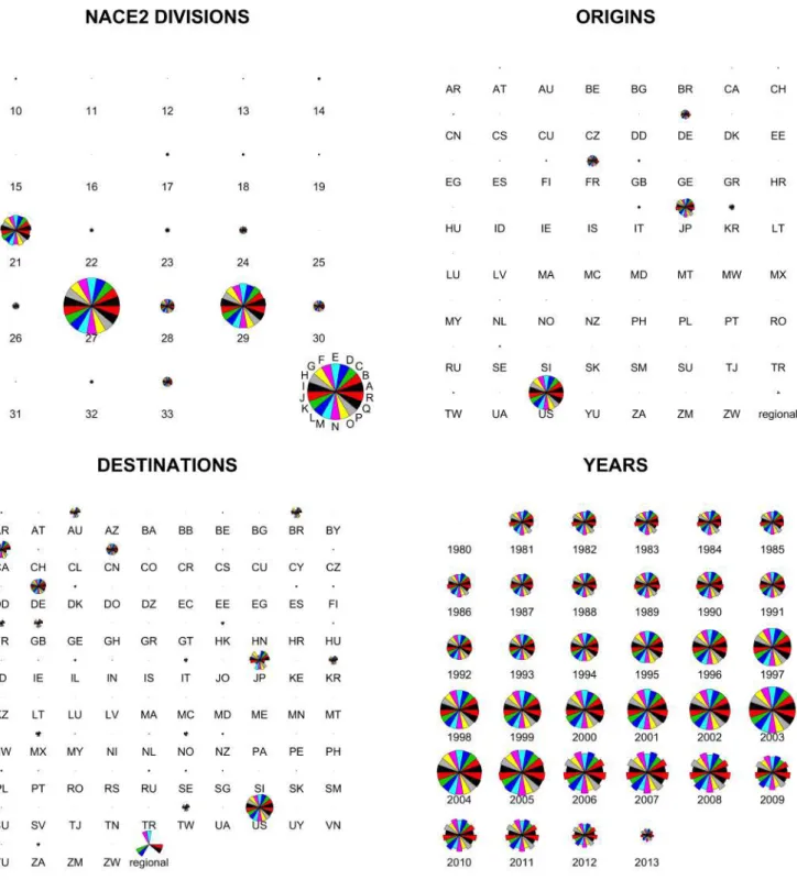
Figure 2 highlights patent-flows as according to the resulting 3 ⇥ 2 ⇥ 3 distinct defini-tions of the dependent variable, each at the aggregate level of distinct NACE2 Divisions of manufacturing, of countries of origin and destination, and time as surfacing in the data. The stars plots shown there visualize the relative size of each category (NACE2 Divisions, countries of origin and destination, years) with respect to the 18 distinct patent-flow mea-sures as compared to all other categories. Different meamea-sures of the dependent variables are represented by different colors. What is highlighted there is a strong overlap in pat-terns, no matter which type of family definition is considered, no matter if PCT and Paris-Convention filings are considered together or whether or not regional applications are excluded. Without loss of generality, we will focus on non-regional subsequent ap-plications according to the Paris Convention and the PCT in the following. These are represented by the radii of the variables A and B (weighted and unweighted count for the single-priority-family), G and D (weighted and unweighted count for the DOCDB-family), and M and N (weighted and unweighted count for the INPADOC-family).
Figure 3 plots the relative frequencies of the selected variables (in logs), and Table 1 supplements this information by a summary of descriptive statistics. The numbers of observations on data on the dependent variable is approximately 3.7 mio observations for each definition. The reported first and second moments show that relative to a Poisson-distributed random variable, the unweighted counts are over-dispersed whereas the fractional counts are under-dispersed. The over-dispersion of the unweighted count may be accounted to many entries equal to one and two in the data whereas the fractional counting smooths the mass-points a bit.
To motivate our later employed empirical specification of the fixed effects, we present an ANOVA for the log-transformed measures of patent-flows in Table 2. As indicated by the reported mean-squares, variation over different divisions of manufacturing as repre-sented by o above explains most of total variation, and variation over countries of desti-nation ( l) second most. Variation over origins and time ( k and t) is less pronounced. Moreover, for the weighted count variation over origins has a higher mean-square as variation over time, which holds for the weighted count vice versa.
We conclude that the patterns of variation in the dependent variable for different family-definitions are highly similar. In the sequel, we will therefore concentrate at the DOCDB-family as the entity defining distinct innovations, and will retain the other
def-initions for robustness checks.21
[Figure 2, Figure 3, Table 1, Table 2]
4.3 Explanatory Variables
4.3.1 Inequaltiy
A measure of inequality Ilt with good data availability is the Gini coefficient measuring the deviation of a country’s income distribution from perfect equality. It takes on values on [0, 1] with a value of 1 implying that one member of the population gets all the income whereas all others get none. A very rich data-set qualitatively oriented towards the gold standard of the Luxembourg Income Study on post- and pre-tax Gini coefficients (GINInetlt and GINImarketlt below) is provided by the Standardized World Income and Inequality data-base (Solt, 2016; SWIID).22 The most recent year covered by the SWIID is 2013.
As a different measure of inequality we use top-income shares. The World Wealth and Income Database (WID; Piketty et. al) provides rich time-series-country-data on income and wealth statistics predominantly constructed from tax records. From this data-base we use information on top-10%, top-5%, and top-1% income shares (TOP10%-sharelt, TOP5%-sharelt, and TOP1%-sharelt as referred to below). As compared to the Gini coefficient, top-income shares immediately highlight whether inequality is attributable to a small rich class. Country-year-coverage for the WID is worse than for the SWIID, and especially poor for the years from 2013 onwards. As according to the latest period covered by the SWIID, we retain the period 2013 for top-income shares but drop future periods.
In Figure 4 we assess the ten distinct marginal relationships that exist among these five inequality measures whenever they are simultaneously observed for a destination l and year t surfacing in our data. The top-income-shares are almost linearly related when considering the three binary relations, and a similar pattern holds for GINInetlt and TOP1%-sharelt. Between GINInetlt and TOP5%-sharelt, and GINInetlt and TOP10%-sharelt share there is an inverse U-shaped relationship between inequality post-taxes and high incomes. Qualitatively this tells us that high levels of inequality post-taxes are most likely accompanied by high top-1% incomes and comparably little mass below at top-10% and top-5% quantiles of the income distribution. Moreover, the observed pattern for the
21Further results for the analysis presented below using the other definitions of the level of the
innova-tion i for defining the dependent variable are available from the authors upon request and will be made available in the Online Appendix to this paper.
22As the SWIID-data were constructed by multiple imputation, point measures of pre- and post-tax
Gini coefficients pre- and post taxes (GINInetltvs. GINImarltin the figure) indicate that for high levels of inequality (approx. > 0.45) there is almost a one-to-one relationship between the Gini coefficients pre- and post-taxes, whereas for low levels of inequality previous to taxes, the reduction in inequality at the level post-taxes is much larger in order of magnitude. Qualitatively, this means that countries in our sample that have low levels of inequality previous to taxes redistribute income more equally post-taxes as compared to countries with a high level of inequality among market incomes initially.
[Figure 4] 4.3.2 Population and GDP
Measures of population and real GDP are obtained from the World Bank’s World De-velopment Indicators (WDI).23 As both variables have strictly positive support, we log-transform them. We will refer to the log of the destination’s population and GDP at time tby log(POPlt) and log(GDPlt) as introduced above, and use log(POPkt) and log(GDPkt) when the origin-country is referred to, respectively. We consider the latter two variables as controls for characteristics of the origin-country of the patent-flow, interpretable as measures of economic size.
In Appendix B we provide some further results on pair-wise correlations among in-equality measures and GDP and population in our data, respectively.24
4.3.3 Measures of Patent Value, Costs, and Strength of Patent Protection There is common sense in the empirical literature that the number of citations a given patent, or a bundle thereof respectively, receives mirrors the economic value of inventions (see Trajtenberg, 1990; Harhoff et. al. 1999; Harhoff et al., 2003; Hall et al., 2005; Abrams and Akcigit; 2013). The study of Trajtenberg (1990) suggests that the social value of an invention is positively correlated with the incidence of subsequent citations. The results presented in Harhoff et. al. (2003) suggest that the number of references to the patent literature as well as the citations a patent receives are positively related to its value. Hall et. al (2005) consider how the market value of the firm as the holder of the patent responds positively to patent citations. More recently, Abrams and Akcigit
23The WDI-series references are SP.POP.TOTL (population) and NY.GDP.MKTP.CN.
24As indicated above, we confirm that there are positive correlations among all inequality measures.
Moreover, the correlation of the share of the top-1% incomes with, population, GDP, and GDP per capita, respectively, are not estimated significantly different from zero, otherwise there is a positive correlation among top-5% and top-10% incomes with population and GDP, whereas there is a negative correlation between Gini coefficients with GDP per capita. This means, that for our data rich countries are likely to have a low level of inequality in terms of Gini coefficients, but a comparably high top-5%/top-10% income share.