RESEARCH OUTPUTS / RÉSULTATS DE RECHERCHE
Author(s) - Auteur(s) :
Publication date - Date de publication :
Permanent link - Permalien :
Rights / License - Licence de droit d’auteur :
Institutional Repository - Research Portal
Dépôt Institutionnel - Portail de la Recherche
researchportal.unamur.be
University of Namur
Understanding the performance of the FLake model over two African Great Lakes
Thiery, W.; Martynov, A.; Darchambeau, F.; Descy, J. P.; Plisnier, P. D.; Sushama, L.; Van
Lipzig, N. P M
Published in:
Geoscientific Model Development
DOI:
10.5194/gmd-7-317-2014
Publication date:
2014
Document Version
Publisher's PDF, also known as Version of record
Link to publication
Citation for pulished version (HARVARD):
Thiery, W, Martynov, A, Darchambeau, F, Descy, JP, Plisnier, PD, Sushama, L & Van Lipzig, NPM 2014, 'Understanding the performance of the FLake model over two African Great Lakes', Geoscientific Model
Development, vol. 7, no. 1, pp. 317-337. https://doi.org/10.5194/gmd-7-317-2014
General rights
Copyright and moral rights for the publications made accessible in the public portal are retained by the authors and/or other copyright owners and it is a condition of accessing publications that users recognise and abide by the legal requirements associated with these rights. • Users may download and print one copy of any publication from the public portal for the purpose of private study or research. • You may not further distribute the material or use it for any profit-making activity or commercial gain
• You may freely distribute the URL identifying the publication in the public portal ? Take down policy
If you believe that this document breaches copyright please contact us providing details, and we will remove access to the work immediately and investigate your claim.
www.geosci-model-dev.net/7/317/2014/ doi:10.5194/gmd-7-317-2014
© Author(s) 2014. CC Attribution 3.0 License.
Geoscientific
Model Development
Understanding the performance of the FLake model over two
African Great Lakes
W. Thiery1, A. Martynov2,3, F. Darchambeau4, J.-P. Descy5, P.-D. Plisnier6, L. Sushama2, and N. P. M. van Lipzig1
1Department of Earth and Environmental Sciences, University of Leuven, Leuven, Belgium
2Centre pour l’Étude et la Simulation du Climat à l’Échelle Régionale (ESCER), Université du Québec à Montréal, Montréal, Canada
3Institute of Geography and Oeschger Centre for Climate Change Research, University of Bern, Bern, Switzerland 4Unité d’Océanographie Chimique, Université de Liège, Liège, Belgium
5Laboratoire d’écologie des Eaux Douces, University of Namur, Namur, Belgium 6Royal Museum for Central Africa, Tervuren, Belgium
Correspondence to: W. Thiery ([email protected])
Received: 25 July 2013 – Published in Geosci. Model Dev. Discuss.: 2 October 2013 Revised: 14 January 2014 – Accepted: 15 January 2014 – Published: 18 February 2014
Abstract. The ability of the one-dimensional lake model
FLake to represent the mixolimnion temperatures for trop-ical conditions was tested for three locations in East Africa: Lake Kivu and Lake Tanganyika’s northern and southern basins. Meteorological observations from surrounding au-tomatic weather stations were corrected and used to drive FLake, whereas a comprehensive set of water temperature profiles served to evaluate the model at each site. Care-ful forcing data correction and model configuration made it possible to reproduce the observed mixed layer seasonality at Lake Kivu and Lake Tanganyika (northern and southern basins), with correct representation of both the mixed layer depth and water temperatures. At Lake Kivu, mixolimnion temperatures predicted by FLake were found to be sensitive both to minimal variations in the external parameters and to small changes in the meteorological driving data, in particu-lar wind velocity. In each case, small modifications may lead to a regime switch, from the correctly represented seasonal mixed layer deepening to either completely mixed or per-manently stratified conditions from ∼ 10 m downwards. In contrast, model temperatures were found to be robust close to the surface, with acceptable predictions of near-surface water temperatures even when the seasonal mixing regime is not reproduced. FLake can thus be a suitable tool to pa-rameterise tropical lake water surface temperatures within mospheric prediction models. Finally, FLake was used to at-tribute the seasonal mixing cycle at Lake Kivu to variations
in the near-surface meteorological conditions. It was found that the annual mixing down to 60 m during the main dry sea-son is primarily due to enhanced lake evaporation and secon-darily to the decreased incoming long wave radiation, both causing a significant heat loss from the lake surface and as-sociated mixolimnion cooling.
1 Introduction
Owing to the strong contrast in albedo, roughness and heat capacity between land and water, lakes significantly influ-ence the surface-atmosphere exchange of moisture, heat and momentum (Bonan, 1995; Mironov et al., 2010). Some ef-fects of this modified exchange are (i) the dampening of the diurnal temperature cycle and lagged temperature response over lakes compared to adjacent land, (ii) enhanced winds due to the lower surface roughness, (iii) higher moisture input into the atmosphere as lakes evaporate at the poten-tial evaporation rate, and (iv) the formation of local winds, such as the lake/land breezes (Savijärvi and Järvenoja 2000; Samuelsson et al., 2010; Lauwaet et al., 2011).
One such region where lakes are a key component of the climate system is the African Great Lakes region. During last decades, the African Great Lakes experienced fast changes in ecosystem structure and functioning, and their future evo-lution is a major concern (O’Reilly et al., 2003; Verburg et
al., 2003; Verburg and Hecky, 2009). To better understand the present lake hydrodynamics and their relation to aquatic chemistry and biology, several comprehensive one-, two- or three-dimensional hydrodynamic models have been devel-oped and applied in standalone mode to lakes in this re-gion (Schmid et al., 2005; Naithani et al., 2007; Gourgue et al., 2011; Verburg et al., 2011). However, to investigate the two-way interactions between climate and lake processes over East Africa, a correct representation of lakes within re-gional climate models (RCMs) and general circulation mod-els (GCMs) is essential (Stepanenko et al., 2013; see Ap-pendix for a list of all acronyms, variables and simulation names). For now, the high computational expense of com-plex hydrodynamic lake models limits the applicability of coupled lake–atmosphere model systems to process studies (Anyah et al., 2006; Thiery et al., 2014). To overcome this issue, the Freshwater Lake model (FLake) was recently de-veloped (Mironov, 2008; Mironov et al., 2010). It offers a very good compromise between physical realism and com-putational efficiency.
As a one-dimensional lake parameterisation scheme, FLake has already been coupled to a large number of numer-ical weather prediction (NWP) systems, RCMs and GCMs (Kourzeneva et al., 2008; Dutra et al., 2010; Mironov et al., 2010; Salgado and Le Moigne, 2010; Samuelsson et al., 2010; Martynov et al., 2012). However, even though it has become a landmark in this respect, FLake has never been thoroughly tested for tropical conditions. Moreover, as sev-eral joint efforts to provide society with climate change in-formation, such as the COordinated Regional climate Down-scaling EXperiment (CORDEX), explicitly focus on the African continent (Giorgi et al., 2009), a correct represen-tation of the African Great Lakes within NWP, RCMs and GCMs becomes of particular importance.
Hence, the main goal of this study is to test – for the first time – the ability of FLake to reproduce the tempera-ture regimes of two tropical lakes in East Africa. Lake Kivu and Lake Tanganyika are selected, as they are the only rift lakes for which both local weather conditions and lake wa-ter temperatures have been monitored for several years. Lake Kivu (Fig. 1b), is a deep meromictic lake, with an oxic mixolimnion seasonally extending down to 60–70 m, below which the monimolimnion is found rich in nutrients and dissolved gases, in particular carbon dioxide and methane (Fig. 2; Degens et al., 1973; Borgès et al., 2011; Descy et al., 2012). Due to the input of heat and salts from deep geother-mal springs, temperature and salinity in the monimolimnion increase with depth (Degens et al., 1973; Spigel and Coul-ter, 1996; Schmid et al., 2005). Moreover, in the deeper lay-ers, vertical diffusive transport is dominated by double dif-fusive convection (Schmid et al., 2010). Lake Tanganyika (Fig. 1c), the first Albertine rift lake south of Lake Kivu, stretches 670 km southwards and, with its 60 km mean width and maximum depth of 1470 m, represents the second largest surface freshwater reservoir on earth (18 880 km3; Savijärvi,
1997; Alleman et al., 2005; Verburg and Hecky, 2009). Lake Tanganyika is also meromictic (Naithani et al., 2007), but its salt content is lower compared to Lake Kivu (Spigel and Coulter, 1996). Lake Kivu and Lake Tanganyika are both characterised by long lake water retention times (∼ 100 yr and ∼ 800 yr, respectively; Schmid and Wüest, 2012; Coul-ter, 1991), hence the impact of riverine in- and outflow is of little importance to the circulation within these lakes.
In this study, lake temperatures were calculated for three sites, one at Lake Kivu and two at Lake Tanganyika, by forcing FLake with observations from surrounding automatic weather stations (AWSs) and subsequently comparing them to observed time series. Besides integrating them with the raw meteorological observations, wind speed measurements and water transparency were also refined within their uncer-tainty range to yield a control simulation representing the correct mixing regime. At each location, FLake was also driven by the re-analysis product ERA-Interim (Simmons et al., 2007). Furthermore, a systematic analysis of FLake’s sen-sitivity to variations in external parameters, meteorological forcing data, and temperature initialisation was conducted. Finally, a study of the surface energy balance allowed at-tributing the mixing regime at Lake Kivu to changes in near-surface meteorological conditions.
2 Data and methods 2.1 AWS data
The Lake Kivu region is characterised by a long dry season extending from June to September, and a wet season from October to May, interrupted by a short dry season around January (Beadle, 1981). Further south in Lake Tanganyika, the dry season sets in one month earlier (Spigel and Coul-ter, 1996; Verburg and Hecky, 2003). Over both lakes, pre-dominantly southeasterly winds reach a maximum during the dry season (Nicholson, 1996; Verburg and Hecky, 2003; Sar-mento et al., 2006).
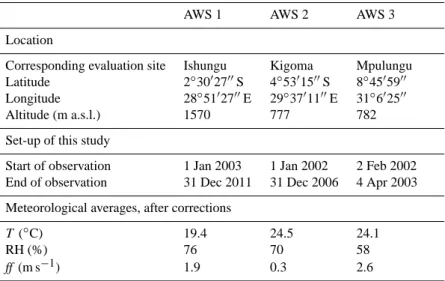
AWS 1 is located on the roof of the Institut Supérieur Pédagogique in Bukavu, Democratic Republic of the Congo, approximately 1 km from the southern border of Lake Kivu and 27 km southwest from the monitoring site in the Ishungu Basin (Fig. 1b). For this study, meteorological observations covering a period of 9 yr (2003–2011) were used. AWS 2 is situated at the Tanzania Fisheries Research Institute in Kigoma, Tanzania, 50 m from the lake shore and 4 km south-east from the evaluation site in Kigoma (Fig. 1c). As such, this station recorded meteorological conditions representa-tive for the northern Tanganyika Basin from 2002 to 2006. Finally, considered as representative for the southern Tan-ganyika Basin, AWS 3 is located at Mpulungu Department of Fisheries, on the lake shore and 8.5 km south of the monitor-ing site of Mpulungu (Fig. 1c). Unfortunately, for this station only 13 months of data (February 2002–April 2003) were
Fig. 1. (a) overview of East Africa with rectangles around Lake Kivu (upper) and Lake Tanganyika (lower), (b) Lake Kivu, (c) Lake
Tanganyika. Surface altitude is shown in m a.s.l.
available. With all three AWSs located on land, one can ex-pect some differences between the measured values and ac-tual meteorological conditions at the sites they aim to repre-sent. However, given the lack of meteorological observations at these locations, it is difficult to assess the degree to which these stations represent their respective evaluation site, ex-cept probably for wind speed measurements (Sect. 2.4). Pos-sibly AWS 3, the most exposed station and located on the lake shore, succeeds best at representing the meteorological conditions of the evaluation site. AWS topographic charac-teristics and meteorological averages are listed in Table 1.
Each AWS records air temperature (T ), pressure (p), wind speed (ff ) and direction (dd), relative humidity (RH) and downward short-wave radiation (SWin) at a single level above the surface, and at an estimated accuracy of ±0.5◦C, ± 1 hPa, ± 5 %, ±3◦, ±3 % and ± 5 %, respec-tively. The measurement frequency is 30 min at AWS 1 and 15 min at AWS 2 and 3, but for the integrations only hourly instantaneous values were retained. Three problems needed to be overcome to prepare the forcing data for the FLake simulations. First, all stations experience frequent data gaps (50 %, 23 % and 37 % of the time at AWS 1, 2 and 3, re-spectively), and gaps are too long to be filled using simple interpolation techniques. This issue was solved by calculat-ing for each hour of the year the climatological average from
available observations and subsequently filling all data gaps with the corresponding climatological value. When no clima-tological value is available for SWin, the value of the previous day was used. At AWS 3, where the time series is too short to obtain climatological values, data gaps were instead filled by the average daily cycle. Second, time series of downward long-wave radiation (LWin), a necessary forcing variable to FLake, are not measured by the AWSs. Hence, they were re-trieved from the ERA-Interim grid point closest to the eval-uation site and subsequently converted from 6-hourly accu-mulated values to hourly instantaneous value.
2.2 FLake model
The one-dimensional FLake model is designed to represent the evolution of a lake column temperature profile and the in-tegral energy budgets of its different layers (Mironov, 2008; Mironov et al., 2010). In particular, the model consists of two vertical water layers: a mixed layer, which is assumed to have a uniform temperature (TML), and an underlying ther-mocline, extending down to the lake bottom (Fig. 2). The temperature-depth curve in the thermocline is parameterised through the concept of self-similarity, or assumed-shape (Kitaigorodskii and Miropolskii, 1970), meaning that the characteristic shape of the temperature profile is conserved
Table 1. Automatic Weather Station (AWS) topographic and meteorological characteristics.
AWS 1 AWS 2 AWS 3 Location
Corresponding evaluation site Ishungu Kigoma Mpulungu Latitude 2◦3002700S 4◦5301500S 8◦4505900 Longitude 28◦5102700E 29◦3701100E 31◦602500 Altitude (m a.s.l.) 1570 777 782 Set-up of this study
Start of observation 1 Jan 2003 1 Jan 2002 2 Feb 2002 End of observation 31 Dec 2011 31 Dec 2006 4 Apr 2003 Meteorological averages, after corrections
T (◦C) 19.4 24.5 24.1
RH (%) 76 70 58
ff (m s−1) 1.9 0.3 2.6
Fig. 2. Water temperature recorded at Ishungu on 21 April 2009 and
corresponding FLake midday temperature profile, the latter with its distinct two-layer structure (mixed layer and thermocline). In-set: temperature (black) and salinity (red) profile representative for the main basin during February 2004, as reported by Schmid et al. (2005). For Lake Kivu, the artificial lake depth set in FLake cor-responds to the mixolimnion depth, hence the monimolimnion has no counterpart in FLake. Note the strong increase in salinity from 60–70 m downwards, i.e. below the mixolimnion.
irrespective of the depth of this layer (Munk and Anderson, 1948). Hence, within the thermocline, temperature at a rela-tive (dimensionless) depth within the thermocline depends only on the shape of the thermocline curve. In turn, this shape is determined only by the temperature at the top and bottom of the thermocline and by a shape factor, describ-ing the curve through a fourth-order polynomial (Mironov, 2008). Additionally, FLake includes the representation of the thermal structure of lake ice and snow cover and (option-ally) also of the temperature of two layers in the bottom
sediments, all using the concept of self-similarity. Without considering ice/snow cover and bottom sediments, the prog-nostic variables computed by the model reduce to: the mixed layer depth (hML), the bottom temperature (TBOT), the wa-ter column average temperature (TMW)and the shape fac-tor with respect to the temperature profile in the thermocline (CT). The mixed layer depth is calculated including effects
of both convective and mechanical mixing, while volumetric heating is accounted for through the net short-wave radia-tion penetrating the water and becoming absorbed accord-ing to the Beer–Lambert law (Mironov, 2008; Mironov et al., 2010). Finally, along with the standalone FLake model comes a set of surface flux subroutines originating from the limited-area atmospheric model COSMO (Consortium for Small-scale Modeling; Doms and Schättler, 2002), hence the components of the surface energy balance are computed fol-lowing the method described by Raschendorfer (2001; see also Doms et al., 2011; Akkermans et al., 2012).
The approach adopted in this study is to test FLake version 1 as close as possible to its native configuration, i.e. how it is operationally used as a lake parameterisation scheme within most atmospheric prediction models. Consequently, modifi-cations in the source code from which the predictions would potentially benefit, such as including time-dependent water transparency, making the distinction between the visible and near-infrared fractions of SWin(each with their own absorp-tion characteristics), improving the parameterisaabsorp-tion of the thermocline’s shape factor, defining a geothermal heat flux, accounting for the effect of bottom sediments, and includ-ing an abyssal layer or diurnal stratification, were not taken into account in this study. Conversely, some of these effects were considered during the lake model intercomparison ex-periment for Lake Kivu (Thiery et al., 2014).
2.3 Water transparency and temperature profiles
In oligotrophic environments such as Lake Tanganyika and Kivu, water transparency is predominantly related to phyto-plankton development, which is usually confirmed by a good correlation between the chlorophyll a concentrations and the downward light attenuation coefficient k (m−1) or related quantity (Naithani et al., 2007; Darchambeau et al., 2014). In FLake, however, k has to be ascribed a constant value. A large measurement set of disappearance depths of the Secchi disk zsd (m) are available for each site (Table 2). zsd were converted to k using the relationship
k =−ln(0.25) zsd
, (1)
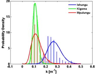
where 0.25 refers to the fraction of incident radiation pen-etrating to the depth at which the Secchi disk is no longer visible. This fraction, differing from one Secchi disk to an-other, was retrieved at Lake Kivu by means of 15 simultane-ous measurements of zsdand the vertical profile of light con-ditions using a LI-193SA Spherical Quantum Sensor, from which k was estimated. For each data set of k, a gamma prob-ability density function was fitted (Fig. 3), from which sub-sequently average ¯k and standard deviation σk were
calcu-lated (Table 2). The higher ¯k observed at Ishungu relative to Kigoma and Mpulungu is caused by the higher phytoplank-ton biomass (represented by chlorophyll a concentrations) in Lake Kivu (2.02 ± 0.78 mg m−3; Sarmento et al., 2012) com-pared to Lake Tanganyika (0.67 ± 0.25 mg m−3; Stenuite et al., 2007). Note that, since an uncertainty remains associated with the exact value of k, its value was allowed to vary within given bounds in the different simulations (see Sect. 2.4).
The evaluation of the FLake simulations was made by the use of 419 conductivity-temperature-depth (CTD) casts col-lected at Ishungu (Lake Kivu), Kigoma (Lake Tanganyika’s northern basin) and Mpulungu (Lake Tanganyika’s south-ern basin; Table 2). At each of these locations, they pro-vide a clear image of the surface lake’s thermal structure and hence mixing regime. While it can be argued that tempera-ture recordings at Ishungu are representative for the whole of Lake Kivu, except Bukavu Bay and Kabuno Bay (Thiery et al., 2014), the same cannot be claimed for Lake Tanganyika, where seasonal variations in wind velocity and internal wave motions cause spatially variant mixing dynamics (Plisnier et al., 1999). This is also apparent from the comparison of the CTD casts of Kigoma and Mpulungu (Sects. 3.2 and 3.3). Consequently, the results of the FLake simulations for Ishungu can be used to study the mixing physics of Lake Kivu (Sect. 3.6), whereas the mixing processes within the whole of Lake Tanganyika cannot be captured by single-column simulations at two sites only.
To ease the intercomparison of the different CTD casts, first, each temperature profile was spatially interpolated to a regular vertical grid with increment 0.1 m using the piece-wise cubic Hermite interpolation technique (De Boor, 1978).
Fig. 3. Comparative histogram of the downward light attenuation
coefficient k (m−1) as observed at Ishungu Basin (Lake Kivu) and Kigoma and Mpulungu stations (Lake Tanganyika). Gamma distribution probability density functions are plotted to the data (R2=0.82, 0.99 and 0.93 for Ishungu, Kigoma and Mpulungu, re-spectively).
Subsequently, the depth of the mixed layer was determined for each cast as the depth with the maximum downward tem-perature change per metre lower than a predefined threshold (−0.03◦C m−1). Whenever the thermal gradient did not ex-ceed this threshold, the lake was assumed to be mixed down to the artificial model depth (see Sect. 2.4). Finally, both tem-perature profiles and mixed layer depths were also tempo-rally interpolated to a grid with increment of one day using the same spline interpolation.
2.4 Model configuration, evaluation and sensitivity
Both in situ meteorological measurements and ERA-Interim data from the nearest grid cell were used to drive FLake in standalone mode (decoupled from an atmospheric model) for three different locations: Ishungu, Kigoma and Mpulungu (Fig. 1). One of FLake’s main external parameters is the lake depth (Mironov, 2008; Kourzeneva et al., 2012b). However, for most of the deep African Great Lakes, their actual lake depth cannot be used, since FLake only describes the mixed layer and thermocline, whereas in reality a monimolimnion is found below the thermocline of these meromictic lakes. Con-sequently, an artificial model lake depth was defined at the maximum depth for which the observed temperature range exceeds 1◦C during the measurement period. When applying
this criterion to the vertically interpolated temperature pro-files, it was found that 60 m is an appropriate artificial depth for Lake Kivu, while for both basins of Lake Tanganyika the seasonal temperature cycle penetrates down to a depth of 100 m. Note that for Lake Kivu, this depth coincides with the onset of the salinity increase, which inhibits deeper mixing (Fig. 2). As a consequence of using an artificial lake depth,
Table 2. Characteristics of the model evaluation sites. Water transparency characteristics are the downward light attenuation coefficient k
(m−1)and its standard deviation σk (m−1). Control run scores are standard deviation σT (◦C), centred root mean square error (RMSEc)
(◦C), Pearson correlation coefficient r and Brier Skill Score (BSS).
Ishungu Kigoma Mpulungu
General characteristics
Lake Kivu Tanganyika (northern basin) Tanganyika (southern basin) Latitude 2◦2002500S 4◦5101600S 8◦4305900S Longitude 28◦5803600E 29◦3503200E 31◦202600E Altitude (m a.s.l.) 1463 768 768 Depth (m) 120 600 120 Number of CTD casts 174 119 126 Water transparency
Number of Secchi depths 163 114 124
Average k (m−1) 0.28 0.11 0.13
σk(m−1) 0.06 0.02 0.05
Minimum k (m−1) 0.15 0.07 0.06
Maximum k (m−1) 0.46 0.17 0.31
Vertically averaged scores for control run
σT (◦C) 0.30 0.70 0.67
(relative to σT ,obs(◦C) 0.32 0.49 0.65
RMSEc(◦C) 0.22 0.59 0.89
r 0.71 0.51 0.05
BSS −0.13 −9.63 −1.81
the bottom sediments module was switched off in all simula-tions. Therewith, a zero heat flux assumption was adopted at the bottom boundary.
At each location, three simulations were conducted. First, FLake was integrated with observed meteorological values and using the average observed value for k (hereafter re-ferred to as “raw”). However, due to the location of AWS 1 and 2 – both surrounded by several buildings and large trees – especially the wind speed values are expected to be underestimated by these stations. Moreover, as the data gap-filling technique averaged out high values for ff, unrecorded high wind speed events were not recreated. Consequently, wind speed recordings at these stations can be considered as a lower bound for the actual ff at the respective eval-uation sites. As a supplementary evidence, wind velocity measurements from a state-of-the-art AWS, newly installed over the lake surface on a floating platform in the main basin and 2 km off the shoreline (AWS Kivu: 1◦4303000S, 29◦1401500E), showed that wind speeds at AWS Kivu were on average 2.0 m s−1higher compared to AWS 1 (from Oc-tober to November 2012, n = 892, root mean square er-ror RMSE = 2.7 m s−1). By applying a constant increase of 2.0 m s−1 to the wind velocities observed at AWS 1, the RMSE between wind velocities from both AWSs reduced to 1.8 m s−1. Since the location of AWS Kivu is much more exposed than the Ishungu Basin – especially given the pre-dominance of southeasterlies over the lake – wind velocities
measured by AWS Kivu provide a definite upper bound for wind velocities in the Ishungu Basin. Hence, a second AWS-driven simulation was conducted wherein wind velocities were allowed to vary within specific upper (from AWS Kivu) and lower (from AWS 1) bounds until the observed mixing regime is reproduced (0.1 m s−1 increment; see Sect. 3.5.2 for another important argument in support of this operation). It was found that at Ishungu, increasing all ff by 1.0 m s−1 resulted in a correct representation of the mixing regime (Sect. 3.1), whereas at Kigoma, ff had to be increased by 2.0 m s−1(Sect. 3.2). At Mpulungu, where the driving AWS is located close by the evaluation site and on the lake shore, the correct mixing regime is already reproduced by the raw integration, and hence no wind speed correction needed to be applied (Sect. 3.3). After correcting for the wind speed, k was varied iteratively between bounds ¯k − σkand ¯k + σk
un-til the best values for the set of model efficiency scores were obtained (see below; hereafter referred to as “control”). This operation led to values of 0.32 m−1, 0.10 m−1and 0.09 m−1 for k at Ishungu, Kigoma and Mpulungu, respectively. Note however that this second correction, restricted by σk
(Ta-ble 2), had little to no impact upon the final model outcome (At Ishungu, for instance, mean mixed layer and water col-umn temperatures differ less than 0.001◦C and 0.04◦C, re-spectively, after this second correction).
Finally, FLake was integrated using ERA-Interim data from the nearest grid cell as forcing. ERA-Interim is a global reanalysis product produced by the European Cen-tre for Medium-Range Weather Forecasts (ECMWF; Sim-mons et al., 2007). It consists of a long-term atmospheric model simulation in which historical meteorological obser-vations are consistently assimilated. Note however that the horizontal resolution of this product is T255 (0.703125◦ or about 80 km), hence a large fraction of each nearest pixel represents land instead of lake. Moreover, only few observa-tions are assimilated into ERA-Interim over tropical Africa, adding to the uncertainty of this product as a source of mete-orological input to FLake. At Mpulungu, the only site where this integration led to a correct representation of the mixing regime (Sect. 3.3), k was again allowed to vary within bounds
¯
k − σk< k < ¯k + σk, with k = 0.09 m−1retained.
In each simulation, lake water temperatures were ini-tialised by the average TML, TWMand TBOTcalculated from the linearly interpolated observed January temperature pro-files (n = 14, 8 and 10 at Ishungu, Kigoma and Mpulungu, respectively). Then, for each location the spin-up time was determined by repeatedly forcing the model with the atmo-spheric time series until the initial TBOTremained constant. This approach was found to be preferable above a spin-up with a constant forcing or with a climatological year (Mironov et al., 2010), as the averaging of the wind speed observations removes extremes which may trigger the deep mixing in these lakes. It was found that, depending on the lo-cation and for the control model configuration, a spin-up time from 9 to 330 yr is needed before convergence is reached.
The ability of FLake to reproduce the observed tempera-ture structempera-ture was tested by comparing FLake’s near-surface and bottom temperature to the corresponding observed val-ues at each location. Note that a depth of 5 m was chosen representative for the surface waters, since (i) CTD casts were generally collected around noon and temperatures in the first metres are therefore positively biased relative to the daily averages, and (ii) FLake does not fully account for the daytime surface stratification because the mixed layer has a uniform temperature. Furthermore, a set of four model effi-ciency scores was computed: the standard deviation σT (◦C),
the centred root mean square error RMSEc(◦C), the Pearson correlation coefficient r and the Brier Skill Score BSS (Nash and Sutcliffe, 1970; Taylor, 2001; Wilks, 2005). The former three calculated scores are visualised together in a Taylor di-agram (Taylor, 2001), enabling the performance assessment of FLake. The RMSEcis given by
RMSEc= v u u t 1 N n X i=1 ((mi− ¯m) − (oi− ¯o))2, (2)
while the BSS is computed according to
BSS = 1 − n P i=1 (oi−mi)2 n P i=1 (oi− ¯o)2 , (3)
with oi the observed (interpolated) water temperature, ¯o
the average observed water temperature, and mi and ¯mthe
corresponding modelled values at time i. Values for BSS range from −∞ (no relation between observed and predicted value) to +1 (perfect prediction). Note that, compared to the variables displayed in a Taylor diagram, the BSS has the ad-vantage of accounting for the model bias.
The sensitivity of the model was evaluated by conducting a number of simulations, each with an alternative configu-ration. In particular, the effects of variations in the external parameter values, the driving data and the initial conditions were investigated in this sensitivity study. Depending on the nature of each sensitivity experiment, different scores are ap-plied to quantify the effect of a specific modification. Details of the different experiments are outlined in Sect. 3.5.
3 Results 3.1 Ishungu
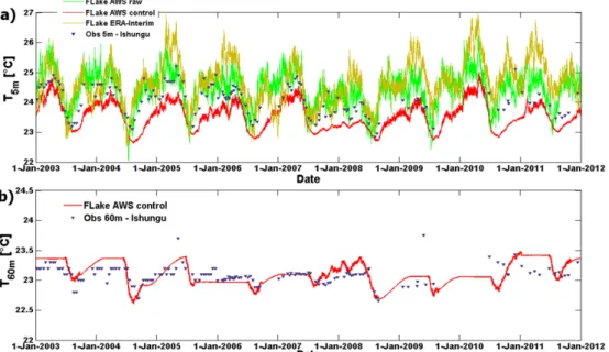
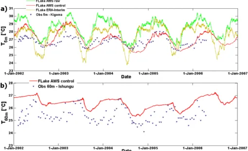
Comparing modelled and observed water temperatures of Lake Kivu near the surface (5 m) shows that the timing of the near-surface seasonal cycle is well represented by the raw, control and ERA-Interim simulations (Fig. 4a). How-ever, whereas it shows a small negative bias compared to the observations, only the control integration grasps the correct magnitude of the seasonal temperature range. The overesti-mation of the temperature seasonality in the raw and ERA-Interim simulations is reflected by 5 m BSS of −0.36 and
−2.13, respectively, compared to only −0.26 for the control case. At a depth of 60 m, both the raw and ERA-Interim inte-gration predict a year-round constant temperature of 3.98◦C, the temperature of maximum density, resulting in a cold bias of about 19◦C. At the bottom, the lake’s thermal structure is reproduced only by the control simulation (BSS = −0.17; Fig. 4b).
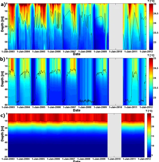
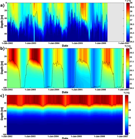
Once a year, during the dry season (from June to August), the mixed layer depth at Ishungu extends down to approxi-mately 60 m. At this depth, the upwelling of deep, saline wa-ters (0.5 m yr−1; Schmid and Wüest, 2012) equilibrates with mixing forces. The result is a strong salinity gradient from 60 m downwards (Fig. 2). During the remainder of the year, stratified conditions dominate, with the mixed layer depth varying between 10 and 30 m (Fig. 5a). The raw simulation does not reproduce this mixing seasonality, but instead pre-dicts permanently stratified conditions and a complete cool-ing down to 3.98◦C from 30 m downwards. On the other hand, with ff corrected for the land effect and k tuned to
Fig. 4. Modelled and observed temperature evolution at Ishungu (Lake Kivu) at (a) 5 m, and (b) 60 m depth. FLake temperatures at 60 m
predicted by the raw and ERA-Interim integration are omitted as they are constant at 3.98◦C.
0.32 m−1, the control simulation closely reproduces the mix-ing regime at Ishungu (Fig. 5b; Table 2). In this case, also the lower stability, indicated by the observations near the end of 2006 and during 2008 and 2009, is captured by this control simulation, although it is somewhat overestimated in 2008 with a predicted year-round mixing down to ∼ 55 m. Note however that, due to the lower stability during these years, the effect on the near-surface water temperatures is limited. Furthermore, also the late onset of the stratification in early 2007 is represented by the model.
Finally, feeding FLake with ERA-Interim-derived near-surface meteorology does not succeed in reproducing the mixing regime. Instead, this simulation predicts permanently stratified conditions and a complete cooling down to 3.98◦C, the temperature of maximum density, from 30 m downwards (Fig. 5c). The low and constant mixed layer depth gener-ates near-surface temperature fluctuations found too strong on seasonal timescales (Fig. 4a). Similar to the raw integra-tion, the inability of the ERA-Interim integration to produce deep mixing is primarily due to the predicted values for the wind velocity, which are 33 % lower compared to the control run average wind velocity and 49 % lower compared to wind speeds from AWS Kivu (measured over the lake surface dur-ing 59 days from October to November 2012). Underlydur-ing reasons for this deviation are (i) the fact that the lake sur-face covers only a fraction of the selected ERA-Interim grid box, and (ii) the higher uncertainty of this product in central Africa owing to the sparse observational data coverage in this region (Dee et al., 2011).
3.2 Kigoma
At Kigoma, the raw and ERA-Interim integrations both pre-dict too high temperature seasonality in the near-surface wa-ter (Fig. 6a). On the other hand, the control experiment clearly displays improved skill at 5 m, especially during 2004 and 2005. At depth, both the raw and ERA-Interim integra-tions obtain a constant 3.98◦C and therewith strongly de-viate from the observations (Fig. 6b). In return, the control simulation again captures the actual conditions much better, even though it slightly underestimates the seasonal tempera-ture range and retains a positive bias between 0 and 2◦C.
Contrary to Lake Kivu, in Lake Tanganyika salinity-induced stratification below 60 m is negligible and seasonal variations in near-surface meteorology are more pronounced (Sect. 3.4). Consequently, the seasonal mixed layer extends further down both during the dry and wet season (Fig. 7a), with mixing recorded down to even 150 m (Verburg and Hecky, 2003) and 300 m (Plisnier et al., 1999). Similar to Ishungu, also at Kigoma the raw simulation does not result in a correct representation of the mixing regime, but pre-dicts permanent stratified conditions and a complete cool-ing along the thermocline. Again, upward correction of ff by 2 m s−1and reducing k to a value of 0.09 m−1brings the model to the correct mixing regime at Kigoma (Fig. 7b; Ta-ble 2). The ERA-Interim simulation predicts permanent strat-ification due to too low wind velocities (Fig. 7c). Note that in both the ERA-Interim and the raw simulations, decreas-ing k from 0.11 m−1 to 0.09 m−1 leads to a regime switch from permanent stratification directly to fully mixed condi-tions (down to the model lake depth), the latter associated with a strong positive temperature bias both near the surface and at depth.
Fig. 5. Lake water temperatures (◦C) at Ishungu (Lake Kivu) (a) from observations, (b) as predicted by the AWS-driven FLake-control, and
(c) as predicted by FLake-ERA-Interim. The black line depicts the mixed layer depth (Sect. 2.3; weekly mean for the simulations). Note the
different colour scaling in (c). The lake water temperatures for the raw simulation are not shown as they strongly resemble the predictions of the ERA-Interim simulation.
3.3 Mpulungu
At Mpulungu, all three experiments capture the magnitude of the seasonal cycle in near-surface temperature and show little to no bias compared to the observations (Fig. 8a). However, also in each simulation the onset of complete mixing lags by around one month and lasts too long compared to observa-tions (Fig. 8a). At 60 m, a similar lag is found (Fig. 8b). Fur-thermore at this depth, the enhanced temperature seasonality of the control integration compared to the raw integration de-picts its improved skill.
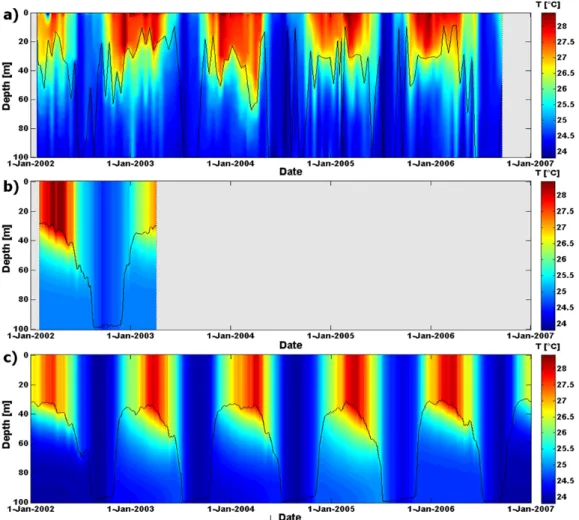
Although the FLake-AWS simulation at Mpulungu spans only 13 months, during this period two stratified periods and one fully mixed season are predicted by the model in both the raw (k = 0.13 m−1)and control (k = 0.09 m−1)set-up, in agreement with observations (Fig. 9a and b; Table 2). With
AWS 3 located on the lake shore (exposed) and relatively close to the evaluation site, no correction of ff was neces-sary, and the mixing regime is correctly represented within the range 0.09 m−1< k <0.22 m−1. Furthermore, also driv-ing FLake with ERA-Interim at Mpulungu leads to a correct representation of the mixing regime (Fig. 9c).
From May to September, persistent southeasterly winds over Lake Tanganyika cause a tilting (downwards towards the north) of the mixolimnion-monimolimnion interface, and therewith generate the upwelling of deep, cold waters at the southern end of the lake (Plisnier et al., 1999). The result-ing breakdown of the stratification appears through the ab-sence of the thermocline at Mpulungu during the dry season (Fig. 9a), whereas at Kigoma, even during this period a weak thermocline remains present (Fig. 7a). Due to its self-similar, one-dimensional nature, FLake does not account for complex
Fig. 6. Modelled and observed temperature evolution at Kigoma (northern basin of Lake Tanganyika) at (a) 5 m, and (b) 60 m depth. FLake
temperatures at 60 m predicted by the raw and ERA-Interim integration are omitted as they are constant at 3.98◦C.
hydrodynamic phenomena such as local upwelling and asso-ciated internal wave phenomena (Naithani et al., 2003), and therefore does not capture this difference between both sites (Figs. 7 and 9). It is likely that this phenomenon may also explain the time lag noticed in all Mpulungu simulations. The hydrodynamic response to the wind stress reinforces the seasonal cycle induced by lake–atmosphere interactions (Sect. 3.6): while the onset of the upwelling accelerates the cooling at the start of the dry season, a cessation of southeast-erly winds in September generates the fast advection of warm mixolimnion waters from the north back towards Mpulungu, inducing a faster restoration of stratification than can be pre-dicted by FLake from lake–atmosphere interactions alone.
3.4 Comparison between sites
A number of differences can be noted between the three lo-cations. First, the average observed 5 m temperature is 2.6◦C
and 2.4◦C lower in Ishungu (altitude 1463 m a.s.l.) compared
to Kigoma and Mpulungu (altitude 768 m a.s.l.), respectively. Second, it can be observed that the water temperature sea-sonality increases with distance from the equator: at 5 m, the maximal observed temperature ranges are 2.4◦C, 2.5◦C and 5.4◦C in Ishungu, Kigoma and Mpulungu, respectively. This is related to differences in near-surface meteorology, since in the Southern Hemisphere at tropical latitudes, a higher distance from the equator coincides with a higher distance from the Intertropical Convergence Zone (ITCZ) during aus-tral winter and thus creates a larger contrast between dry and wet season (Akkermans et al., 2014).
Third, although the average latent heat flux (LHF) is very similar at Ishungu (88 W m−2) and Kigoma (86 W m−2), it increases by 56 % at Mpulungu (134 W m−2) during the respective measurement periods. Extrapolating the average LHF at Ishungu to the entire Lake Kivu surface (estimated by the control simulation and using a surface area of 2370 km2; Schmid and Wüest, 2012) leads to a preliminary estimate of the total annual evaporative flux of 2.6 km3yr−1for the pe-riod 2003–2011. Note that, based on calculations from Bul-tot (1971), Schmid and Wüest (2012) estimate a Bul-total an-nual evaporation of 3.0–4.0 km3yr−1for Lake Kivu. Analo-gously, extrapolating the average LHF computed for Kigoma to the northern Tanganyika Basin (17 572 km2; Plisnier et al., 2007) leads to a preliminary estimate of 18.8 km3yr−1 for the total annual evaporation from the northern basin. At Mpulungu, where the control simulation predicts an average LHF of 133 W m−2 for the measurement period, extrapola-tion yields a total annual evaporaextrapola-tion of 23.8 km3yr−1from the southern basin (14 173 km2; Plisnier et al., 2007). For the ERA-Interim simulations, the average LHF amounts up to 114 W m−2 (25.3 km3 yr−1)at Kigoma and 138 W m−2 (24.7 km3yr−1) at Mpulungu. Note that Verburg and An-tenucci (2010) computed a lake-wide evaporation amount-ing up to 63 km3yr−1, when assuming a total surface area of 31 745 km2 for Lake Tanganyika. The annual lake-wide evaporation estimates from the control and ERA-Interim simulations are only 65 % (42.6 km3) and 80 % (50.1 km3) of this value, respectively. Possible explanations for this dis-crepancy are (i) the different method used to compute the latent heat flux, (ii) differences in the quality and length of the meteorological time series, and (iii) the period of observation (1994–1996 versus 2002–2003 and 2002–2006,
Fig. 7. Lake water temperatures (◦C) at Kigoma (northern basin of Lake Tanganyika) (a) from observations, (b) as predicted by the AWS-driven FLake-control, and (c) as predicted by FLake-ERA-Interim. The black line depicts the mixed layer depth (Sect. 2.3; weekly mean for the simulations). Note the different colour scaling in (c).
respectively). Especially the latter effect is potentially rele-vant, given the influence of large-scale climate oscillations such as the El Niño–Southern Oscillation (ENSO) on the regional climate (Plisnier et al., 2000) and the contrasting ENSO indices found for both periods (La Niña years versus El Niño years). Further research will aim at quantifying un-certainties associated with lake-wide evaporation estimates for tropical lakes.
Results from the AWS control simulations show that FLake successfully incorporates these differences between the sites, since the model, through the differences in forcing and configuration, successfully represents the thermal struc-ture of both Lake Kivu and Lake Tanganyika and discerns the differences between the two basins within Lake Tanganyika.
3.5 Sensitivity study
Originally designed for implementation within NWP sys-tems or climate models, FLake requires information on lake depth and water transparency (downward light attenuation coefficient) for each lake within its domain. But despite re-cent efforts to gather and map lake depth on a global scale (Kourzeneva, 2010; Kourzeneva et al., 2012a), in East Africa information on lake depth and water transparency is only available for the largest lakes, adding uncertainty to FLake’s outcome when it is applied to the entire region. Furthermore, the effect of the forcing data source – e.g. originating from an AWS, a reanalysis product or RCM output – and its as-sociated quality might significantly affect the outcome of a simulation. As RCMs and standalone lake models are being applied to increasingly remote lakes, the need to consider this data quality issue grows (Martynov et al., 2010). Finally, in
Fig. 8. Modelled and observed temperature evolution at Mpulungu (southern basin of Lake Tanganyika) at (a) 5 m, and (b) 60 m depth.
the absence of initialisation data, several approaches to lake temperature initialisation and spin-up have been applied in the past (Kourzeneva et al., 2008; Mironov et al., 2010; Bal-samo et al., 2012; Hernández-Díaz et al., 2012; Rontu et al., 2012). Hence, a systematic study of the sensitivity of the model to different sources of error is appropriate. Hereafter, results of FLake’s sensitivity to variations in (i) external pa-rameters, (ii) meteorological forcing data, and (iii) tempera-ture initialisation are presented. Note that each set of the fol-lowing tests was conducted starting from the Lake Kivu con-trol simulation (Sect. 3.1). However, the same experiments have been conducted for Kigoma and Mpulungu as well, and revealed very similar responses to the imposed changes.
3.5.1 External parameters
The first set of model sensitivity tests was conducted to in-vestigate FLake’s sensitivity to changes in the model’s exter-nal parameters. Using a set of four model efficiency scores (Sect. 2.4), the impact of setting the model lake depth to a relatively shallow 30 m (SHA) or a relatively deep 120 m (DEE), and setting k to the highest (KHI) or lowest (KLO) observed value at Ishungu (Table 2) was quantified. σT,
RMSEcand r calculated at three depths (5 m, 30 m and 60 m, respectively) are visualised in Taylor diagrams (Fig. 10). Fur-thermore, note that we also investigated the sensitivity of FLake to changes in the fetch, by conducting a set of sim-ulations with the fetch varying between 1 and 100 km, re-spectively (the value in all other simulations is 10 km). It was found, however, that for Lake Kivu, FLake exhibits only little sensitivity to modifications in this parameter.
At 5 m depth, the different sensitivity experiments produce similar values for RMSEc, r, and BSS (not shown). The only score for which the control simulation outcompetes the other members is σT, suggesting that in this case seasonal
tempera-ture variability is closest to reality. At 30 m, some changes to this pattern can already be noticed (Fig. 10b). Most notably, for the SHA test case predictive skill significantly decreases. For this test, FLake predicts fully mixed conditions down to 30 m most of the time, except during the 2005, 2007 and 2009 rainy seasons, when mixing down to 10 m is predicted. How-ever, only at 60 m do the differences fully emerge, with a clear reduction in predictive skill for the simulations with k decreased (increased) to the lowest (highest) observed values at Ishungu. Higher water transparency leads to deeper mix-ing, as solar radiation penetrates down to the interface be-tween mixed layer and thermocline and therewith enhances
hML. Note that for the more transparent Lake Tanganyika, FLake’s sensitivity to changes in k is even more important. There, a change of less than 1σ away from the average ob-served k already led to a switch from permanently mixed conditions to a continuously stratified regime.
3.5.2 Forcing data
In a second set of experiments, FLake’s sensitivity to changes in forcing variables was investigated. Starting from the con-trol simulation at Ishungu, values for T , RH, ff and LWin were varied in pairs between bounds oi−2σ to oi+2σ ,
with oi the actual observed value at time step i, and σ the
standard deviation of a given variable (see also Thiery et al., 2012). Standard deviations for T , RH, ff and LWin are 2.4◦C, 14 %, 1.7 m s−1and 18 W m−2, respectively. The per-turbation increment was 0.4 × σ in each experiment. The
Fig. 9. Lake water temperatures (◦C) at Mpulungu (southern basin of Lake Tanganyika) (a) from observations, (b) as predicted by the AWS-driven FLake-control, and (c) as predicted by FLake-ERA-Interim. The black line depicts the mixed layer depth (Sect. 2.3; weekly mean for the simulations). Results in (c) were obtained with k = 0.09 m−1.
vertically averaged BSS for water temperature calculated per metre depth for 2003–2011 after this pairwise perturbation (Fig. 11) allowed for the selection of the main environmen-tal variables controlling hMLin tropical conditions. Sensitiv-ity experiments for p and SWin are not shown, the former since FLake was found to be not sensitive to this variable, the latter since its high standard deviation (252 W m−2)led to unrealistic perturbations. To overcome this issue, an addi-tional experiment was conducted wherein the SWinand LWin time series were perturbed by the respective standard devia-tions of their daily means (σdm, with values of 35 W m−2and 12 W m−2, respectively; Fig. 12).
For Lake Kivu, FLake results reveal a marked sensitiv-ity to variations in wind speed (Fig. 11a and b). Generally, when wind velocities increase (decrease), mechanical mix-ing reaches deeper (less deep) into the lake, causmix-ing a coolmix-ing (warming) of the mixed layer for the same energy budget. For Lake Kivu, however, at some point the increased wind veloc-ity provokes a regime switch from seasonally mixed condi-tions to (almost) permanently mixed condicondi-tions. This switch,
illustrated by the sharp decrease in BSS in Fig. 11a, b along the ff axis, is already reached before ff is enhanced by 0.4σ . Similarly, only slightly decreasing ff already leads to a sharp switch to the permanently stratified regime. Increasing (de-creasing) T and RH by their respective σ equally contributes to higher (lower) mixed layer temperatures, which in turn en-hances (reduces) stratification (Fig. 11c). Again, the verti-cally averaged BSS depicts the switch to both other regimes: a sharp transition to permanent stratification for increased T and RH and a gradual transition to fully mixed conditions for lower T and RH. A similar sensitivity is found when testing for LWin, although FLake seems less sensitive to variations in this variable (Fig. 11d). When comparing SWinand LWinfor perturbations of the order of their respective σdm(Fig. 12), it can be noted that fairly large perturbations are needed to provoke a regime switch, and that such a switch is provoked more easily by modifying SWinthan LWinby their respective
σdm. Note that when combined in pairs, errors may compen-sate each other and still generate adequate model predictions, as is the case when, e.g. simultaneously reducing ff and T by
Fig. 10. Taylor diagram indicating model performance for water temperature at (a) 5 m, (b) 30 m and (c) 60 m depths for different external
parameter values at Ishungu (January 2003–December 2011). Standard deviation σT (◦C; radial distance), centred root mean square error
RMSEc (◦C; distance apart) and Pearson correlation coefficient r (azimuthal position of the simulation field) were calculated from the
observed T-profile interpolated to a regular grid (1 m increment) and corresponding midday FLake profile. OBS: observations, CTL: control, SHA (DEE): model lake depth set to and 30 m (120 m), KHI (KLO): downward light attenuation coefficient k set to the highest (lowest) observed value at Ishungu. Note that model performance indicators at 60 m cannot be calculated for the SHA integration.
one respective σ , or increasing LWinwhile decreasing RH by one respective σ .
Finally, for each variable in this experiment, one can also derive an uncertainty range for which FLake predicts the cor-rect mixing regime. With a vertically averaged BSS thresh-old set to −20, the range width of wind velocities for which a correct mixing regime is predicted is 0.7 m s−1around the actual observed values of the control run (Fig. 11a). For RH,
T, LWin and SWin, this range is 17 %, 2.0◦C, 50 W m−2 and 42 W m−2, respectively. While for the latter four vari-ables, collecting in situ measurements within these uncer-tainty bounds is feasible, clearly, the room for manoeuvre in case of wind velocity measurements is very small. Con-sequently, the need for reliable wind velocities is critical to have FLake predicting the right mixing conditions over deep tropical lakes. Note that this is also the reason why wind speed was selected as the forcing variable to correct (Sect. 2.4). In return, when the same computation is con-ducted for the 5 m BSS instead of the vertically averaged BSS, the narrow band widens to 3.4 m s−1(even with a 5 m BSS threshold set to only −2, the acceptable uncertainty range is still 2.0 m s−1). Thus, in cases where the primary interest of the FLake application is the correct representation of near-surface water temperatures, the need for very high ac-curacy wind velocity measurements becomes less pressing.
This has implications for the applicability of FLake to the study of tropical lake–climate interactions. When FLake is interactively coupled to an atmospheric model, it may very well be that, e.g. the near-surface wind velocities serving as input to FLake will not fall within the narrow range for which it predicts a correct mixing regime. However, the only FLake variable which directly influences the atmospheric boundary layer is TML, the variable from which the exchange of water and energy between the lake and the atmosphere
are computed. In this study, TML predictions were found to be robust, even when modelled TBOT values are biased. We may therefore suppose that for tropical conditions, a coupled model system will not be much affected by the strong sen-sitivity of FLake’s deepwater temperatures to, for instance, wind speed values.
3.5.3 Initial conditions
The third set of experiments at Lake Kivu was designed to test the model to different initial conditions. In the control simulation, FLake was initialised with the average mixed layer, total water column and bottom temperatures calculated from the January CTD profiles (n = 14), after which spin-up cycles were repeated until convergence is reached. Sensi-tivity experiments encompassed a simulation with the same initialisation but excluding spin-up (CES), a fully mixed (i.e. down to 60 m depth) water column initialisation includ-ing (MIS) or excludinclud-ing spin-up (MES), and a stratified wa-ter column excluding spin-up (SES). By setting the initial mixed layer depth to 60 m and the lake water temperature to 28◦C, full mixing was imposed, whereas permanently strat-ified conditions were obtained by setting the initial mixed layer depth to 8 m, TMLto 23.5◦C and Tbotto 4◦C (compa-rable to Hernández-Díaz et al., 2012; Martynov et al., 2012). Note that a stratified initialisation including spin-up is omit-ted, since downward heat transport within the thermocline can only occur through molecular diffusion in this case, and hence would require millennia-scale spin-up time. Again,
σT, RMSEc, and r were calculated and visualised for three depths (Fig. 13).
First, it can be noted that omitting spin-up in the optimal simulation (CES) has only limited, though negative, influ-ence on the predictive skill. This shows that when a reli-able initial CTD profile is availreli-able, spin-up has some, but
Fig. 11. Vertically averaged Brier Skill Scores (BSS) of water temperature profiles (0–60 m; 1 m vertical increment) at Ishungu from 4
sensitivity experiments, wherein pairs of forcing variables recorded at AWS 1 were perturbed by proportions of their respective standard deviations σ . Perturbed forcing variables are wind velocity (ff), Relative humidity (RH), air temperature (T ) and incoming long-wave radiation (LWin). Generally, values for BSS range from +1 (perfect prediction) to −∞ (no relation between observation and prediction).
Here, BSS below −100 are set to −100. Permanently stratified (STRAT) and fully mixed conditions down to 60 m (MIXED) are indicated.
Fig. 12. Vertically averaged Brier Skill Scores (BSS) of water
tem-perature profiles (0–60 m; 1 m vertical increment) at Ishungu from a set of simulations with SWinand LWinperturbed by proportions
of their respective standard deviations of daily mean values (σdm).
only little added value. More interestingly, however, is the fact that a fully mixed and artificially warm initialisation with spin-up (MIS) succeeds very well in reproducing the thermal structure of Lake Kivu. Within 9 spin-up years, the
complete mixing allows for an efficient heat release until the regime switches to the expected pattern. Since the model is allowed to spin-up until convergence is reached, the selec-tion of the initial water column temperature does not influ-ence the model performance, as long as it is chosen artifi-cially warm. However, without spin-up (MES), this advan-tage vanishes and results have limited skill, since the lake has been initialised too warm. Alternatively, when offline spin-up of lake temperatures is not feasible within the cospin-upled model system, imposing permanently stratified conditions by means of a 4◦C lake bottom (SES) becomes an option, given
the acceptable results near the lake surface even though the thermal structure is not reproduced. Note that this was the approach adopted for the CORDEX-Africa simulations con-ducted with the Canadian Regional Climate Model version 5 (Hernández-Díaz et al., 2012; Martynov et al., 2012). Hence, for coupled FLake-atmosphere simulations over regions with no initialisation information available, a fully mixed, artifi-cially warm initialisation appears to be the best option, but only if offline lake temperature spin-up is applied; otherwise an imposed, permanently stratified regime is to be preferred.
3.6 Mixing physics at Lake Kivu
Studying the seasonal variations in the near-surface mete-orological conditions and in the surface energy balance of
Fig. 13. Taylor diagram indicating model performance for water temperature at (a) 5 m, (b) 30 m and (c) 60 m depths for different initial
conditions at Ishungu (January 2003–December 2011). OBS: observations, CTL: control, CES: control excluding spin-up, SES: stratified excluding spin-up, MIS (MES): mixed warm initialisation including (excluding) spin-up. Note that SES is omitted at 60 m given its strong deviation from observations there.
the Ishungu control experiment allows us to attribute the seasonal mixing cycle for Lake Kivu. On the one hand, even though ff depicts some seasonality (Fig. 14a), neither
ff nor T influence the seasonality of the mixed layer depth
at Ishungu. First, a comparative histogram of corrected ff binned per month (1 m s−1bin width; not shown) reveals that the probability of occurrence of stronger winds (ff > 5 m s−1)
is lower from April to July, adding to the hypothesis that higher wind velocities are not responsible for the deepen-ing mixed layer depth durdeepen-ing the dry season. This is con-firmed by FLake, who attributes the mixed layer deepening at the start of the dry season to convection rather than wind-driven mixing. Moreover, when conducting the Ishungu con-trol simulation with the seasonality removed from ff, the pre-dicted water temperatures are almost identical to the control simulation. This indicates that the ff seasonality also has no major influence on the convective-driven mixing.
On the other hand, in contrast to ff and T , RH and LWin both show a clear seasonality, with 3-monthly averages 13 % and 11 W m−2, respectively, lower for the June–August pe-riod compared to December–February pepe-riod. Their monthly average values show that the seasonal RH cycle lags the LWin cycle by about one month, but they confirm the strong drop during the main dry season (Fig. 14b). Here, two effects enforce each other to reduce the amount of energy avail-able to stratify the lake surface. First, as a consequence of reduced cloudiness during the dry season, less thermal ra-diation reaches the surface. This, in turn, causes a higher upward net long-wave radiation flux (LWnet)from May to July (Fig. 15). Second, more importantly, while a moisture climate close to saturation inhibits significant evaporation throughout most of the year, the RH drop during the dry sea-son opens a larger potential to evaporation. This effect can be noted in the monthly average anomalies of the surface energy balance components, wherein the LHF shows a marked pos-itive anomaly in months with low RH (Fig. 15). The energy
Fig. 14. Monthly averages for 2003–2011 of (a) wind velocity
ff (m s−1)and air temperature T (◦C); (b) relative humidity RH
(%) recorded at Automatic Weather Station (AWS) 1 and incoming long-wave radiation LWin(W m−2)from ERA-Interim. Note the
different y axes increments.
consumed for evaporating is no longer available to heat the water surface. Thus, lower thermal radiation input and espe-cially enhanced evaporation cause a significant reduction in the amount of energy available to heat near-surface waters.
Fig. 15. Deviation of the monthly average of the surface energy
balance components from its long-term mean (W m−2)at Ishungu, 2003–2011, calculated by FLake’s surface flux routines. Compo-nents are net short-wave radiation (SWnet), net long-wave radiation
(LWnet), sensible heat flux (SHF), latent heat flux (LHF) and
sub-surface conductive heat flux (Q).
To compensate for this surface heat deficit, the upward sub-surface conductive heat flux enhances, in turn generating a drop in the mixed layer temperature.
From mid-June onwards, near-surface water temperatures become low enough for the deep mixing to set in. Near the end of the dry season, from mid-August onwards, evapo-ration rates dramatically drop, causing the warming of sur-face waters from mid-September forward. Note that whereas enhanced solar radiation penetration into the lake is absent during the first phase of the dry season, near the end it slightly contributes to the restoration of surface stratification (Fig. 15). Overall, monthly variations in downward short-wave radiation (SWin)seem to have only little effect on the mixed layer seasonality. Possibly, the interplay of astronomic short-wave radiation variability (with less short-wave radia-tion reaching the top of the atmosphere during the dry sea-sons) and seasonally varying cloud properties (Capart, 1952) balances out the amount of short-wave radiation reaching the surface on monthly timescales.
4 Discussion and conclusions
In general, this study shows that the thermal structure of the mixed layer and thermocline of two African Great Lakes can be reproduced by the FLake model. In particular, the seasonality of the near-surface water temperatures of Lake Kivu and Lake Tanganyika is well captured by the AWS-driven simulations when choosing appropriate values for the wind speed correction factor and k within their uncertainty range. Moreover, FLake was found capable of reproducing
the observed interannual variability, as well as the observed differences between the three sites. The spatial variability is accounted for through varying lake characteristics and me-teorological conditions associated with different surface alti-tude and distance from the equator. At Ishungu, a study of the near-surface meteorology and surface heat balance was used to attribute seasonal mixing cycle of Lake Kivu. Rather than seasonal variations in wind velocity or air temperature, the marked dry season decrease of the incoming long-wave ra-diation and, especially, relative humidity with an associated evaporation peak, reduce the amount of energy available to induce surface stratification.
The near-surface water temperatures were found to be quite robust to changes in the model configuration. If the observed mixing regime is not reproduced, 5 m temperature predictions deteriorate compared to the control integration, but are relatively little affected. Hence, FLake can be con-sidered an appropriate tool to study the climatic impact of lakes in the region of the African Great Lakes. In contrast, an accurate representation of the thermal structure of the mixed layer and thermocline depends strongly on the reliability of meteorological forcing data and a correct choice of model lake depth and water transparency. Slight differences in ex-ternal parameters, and uncertainties associated with the mete-orological forcing data (for instance related to measurement or atmospheric model uncertainty, or to the representativity of the data for over-lake conditions) may already lead to a switch from the observed regime of seasonal mixed layer deepening to either the permanently stratified or the fully mixed regime.
One important reason for this delicate balance found at Lake Kivu is the absence of an abyssal layer in FLake. In re-ality, the abyssal layer acts as a heat reservoir which buffers potential changes in bottom temperature. FLake, on the con-trary, assumes a zero heat flux at the water–sediment inter-face (sediment routine switched off) or at the lower bound of the active sediment layer (sediment routine switched on). In cases where an artificial lake depth is set, this assumption can lead to unrealistic temperature fluctuations near the bottom. Hence, a future development could be to include an abyssal layer in FLake (Mironov et al., 2010).
A second issue is the reliability of water transparency val-ues. Even in more studied areas, information on the spatial and temporal variability of water transparency is mostly lack-ing (Kirillin, 2010; Kourzeneva et al., 2012b; Rontu et al., 2012). Therefore, the first need is to collect more observa-tions of k and to gain more insight into the relaobserva-tionship be-tween water transparency and seasonal mixing cycles in deep tropical lakes. In the future, FLake could then also be adapted to account for these seasonal fluctuations in k.
When applying FLake over regions containing warm deep lakes, values for the external parameters thus need to be considered carefully. This is especially true when FLake is coupled to NWP, RCM or GCM models, since the mete-orological forcing data are potentially biased in that case.
When setting up a climate or NWP simulation with interac-tive lakes, moreover, no information on the lake’s initial con-ditions is available. In that respect, this study clearly shows that it is advisable to initialise all lakes with an artificially warm, uniform temperature and to allow for a considerable offline spin-up of the lake module. When such an offline lake spin-up is not feasible, initialising FLake with stratified con-ditions and an artificially low bottom temperature of 4◦C is to be preferred.
To conclude, the goal of this study was to assess the qual-ity of lake temperature predictions by FLake when applied to tropical lakes. This was done through a number of sim-ulations for three locations in the African Great lakes re-gion: Ishungu (Lake Kivu), Kigoma (northern basin of Lake Tanganyika) and Mpulungu (southern basin of Lake Tan-ganyika). Results show that FLake is able to well represent the mixing regime at these different locations, however only when the model was carefully configured and allowed to spin-up over a considerable period. When input data quality is an issue, or the model is poorly configured, model results tend to deviate from observations towards the deep in large tropical lakes.
Code availability
FLake is freely available under the terms of the GNU Lesser General Public License (http://www.gnu.org/licenses/lgpl. html). The model source code, external parameter data sets and a comprehensive model description can be obtained from the official FLake website (http://www.lakemodel.net), along with pre-processed meteorological forcing for several test cases.
Appendix A
Table A1. Acronyms and variable names
AWS Automatic Weather Station BSS Brier Skill Score []
CORDEX Coordinated Regional climate Downscaling Experiment
COSMO Consortium for Small-scale Modeling control FLake simulation with ff and k corrected
CT Shape factor with respect to the temperature
profile in the thermocline []
CES Same as control, but excluding spin-up CTD Conductivity-Temperature-Depth cast
dd Wind direction [◦]
DEE Same as control, but with lake depth set to 120 m
ENSO El Niño–Southern Oscillation
ERA-Interim Reanalysis product from January 1979 on-ward, produced by the European Centre for Medium-Range Weather Forecasts
ff Wind velocity [m s−1] FLake Freshwater Lake model GCM General Circulation Model
hML Mixed layer depth [m]
ITCZ Intertropical Convergence Zone
k Downward light attenuation coefficient [m−1]
KHI Same as control, but with k set to 0.46 m−1 KLO Same as control, but with k set to 0.15 m−1 LHF Latent heat flux [W m−2]
LWin Downward long-wave radiation [W m−2]
LWnet Net long-wave radiation [W m−2]
MES Same as control, but initially fully mixed and excluding spin-up
MIS Same as control, but initially fully mixed
n Number of observations [] NWP Numerical Weather Prediction
p Air pressure [Pa]
r Pearson correlation coefficient []
raw FLake simulation with observed meteorol-ogy and k
RCM Regional Climate Model RH Relative humidity [%]
RMSE root mean square error [respective unit] RMSEc Centred root mean square error [respective
unit]
σ Standard deviation [respective unit] SES Same as control, but initially strongly
strat-ified and excluding spin-up
SHA Same as control, but with lake depth set to 30 m
SWin Downward short-wave radiation [W m−2]
T Air temperature [◦C]
TBOT Bottom temperature [◦C]
TML Mixed layer temperature [◦C]
TMW Water column average temperature [◦C]
zsd Disappearance depths of the Secchi disk
[m]
Acknowledgements. We would like to thank Dmitrii Mironov for
the helpful discussions on the modelling of tropical lakes and the Institut Supérieur Pédagogique in Bukavu for supplying data of AWS 1. We also sincerely thank the Editor and the two anonymous reviewers for their constructive remarks. This work was financially and logistically supported by the Research Foundation – Flanders (FWO) and the Belgian Science Policy Office (BELSPO), the latter through the research projects EAGLES and CHOLTIC.