Nonlinear seismic response of the soil-structure system : experimental analyses

(1)

HAL Id: tel-01282658

https://tel.archives-ouvertes.fr/tel-01282658

Submitted on 4 Mar 2016

HAL is a multi-disciplinary open access archive for the deposit and dissemination of sci-entific research documents, whether they are pub-lished or not. The documents may come from teaching and research institutions in France or abroad, or from public or private research centers.

L’archive ouverte pluridisciplinaire HAL, est destinée au dépôt et à la diffusion de documents scientifiques de niveau recherche, publiés ou non, émanant des établissements d’enseignement et de recherche français ou étrangers, des laboratoires publics ou privés.

Johanes Chandra

To cite this version:

Johanes Chandra. Nonlinear seismic response of the soil-structure system : experimental analyses. Earth Sciences. Université de Grenoble, 2014. English. �NNT : 2014GRENU023�. �tel-01282658�

(2)

THÈSE

Pour obtenir le grade de

DOCTEUR DE LUNIVERSITÉ DE GRENOBLE

Spécialité : Sciences de la Terre, lUnivers et lEnvironnement Arrêté ministériel : 7 août 2006

Présentée par

Johanes CHANDRA

Thèse dirigée par Philippe GUEGUEN

préparée au sein de lInstitut des Sciences de la Terre dans l'École Doctorale Terre, Univers, Environnement

Analyses expérimentales de la

réponse sismique non-linéaire

du système sol-structure

Thèse soutenue publiquement le 28 Octobre 2014, Devant le jury composé de :

Pr. Arezou MODARESSI

Ecole Centrale Paris, Rapporteur

Pr. Roberto PAOLUCCI

Politecnico di Milano, Rapporteur

Pr. Alain PECKER

Ecole des Ponts ParisTech, Examinateur

Pr. Olivier COUTANT

ISTerre, Univ. Joseph Fourier, Grenoble, Président

Dr. Philippe GUEGUEN

ISTerre, Univ. Joseph Fourier, Grenoble, Directeur de thèse

Dr. Luis Fabian BONILLA (invité)

(3)

(4)

Foreword

I never forget the joy when I read Philippes letter as the beginning of my PhD journey. I keep that joy as my motivation that drove me through all the up and down moments during these three years. I am grateful to have Philippe Guéguen as my mentor who has been patiently guiding me through the entire process. I really could not ask for a better supervisor! I would like to thank as well, Fabian Bonilla, for his enlightening collaboration, and Jamie Steidl which gave me a glimpse of the fieldwork reality.

I would like to thank Pierre-Yves Bard, Jean-François Semblat, Fernando Lopez Caballero, Céline Gélis, Emmanuel Chaljub and other heaps of names that I cannot all list here for all the fruitful discussions that we had. I would also like to thank Roberto Paolucci and Arezou Modaressi for their time reading and commenting this manuscript. I thank the aforementioned juries as well as Alain Pecker and Olivier Coutant for assisting and being part of the defense process.

I would like to express my gratitude to these following names for supporting me, becoming my family, and sharing this process: Afifa Imtiaz, Ismaël Riedel, Olga Ktenidou, Hilal Tasan, Claudia Aristizabal, Zahra Mousavi, Anne Obermann, Amir Asnaashari, Haskell Sie, Maria E. Suryatriyastuti, Jessica Sjah, PPI Grenoble, all ISTerre; To them who proofread my manuscript without burning them: Haskell Sie, Eleanor Bakker, Paul Wellington, and Olga Ktenidou; and of course all the names that again I could not list here without making this acknowledgement thicker than the manuscript itself. To Philippe Perrin who bore all the craziness at the end of the journey without losing his sanity!

I do not forget my family who is always in my heart despite this 11,361 km distance, for all their prayers and supports: Siauw Jonny Sarsono, Khoe Chun Lan, Christian Chandra, and Michael Chandra.

I have been blessed! Johanes

(5)

(6)

General Introduction

The earth consists of several moving tectonic plates. While moving, these plates store strain energy, and as the shear stress on these fault planes passes the shear strength of the rock along the fault, this strain energy is released as what we known as earthquake. These earthquakes are one of the most detrimental natural disasters that mankind face. Depending on its level, the energy release can generate death and destruction. For example, during the period between 2000 and 2010, earthquakes have contributed to the death of approximately 699,000 people (Holzer and Savage, 2013). Some recent noteworthy earthquakes include the 2004 Sumatra-Andaman earthquake (Mw = 9.1) that killed more than 220,000 people; the 2010 Haiti earthquake (Mw = 7.0) with around 316,000 deaths; and the 2011 Tohoku earthquake (Mw = 9.0) that killed more than 22,000 people.

When discussing global risk management, it is important to understand the definition of risk itself. Risk is not only related to hazard, but is also the product of vulnerability and exposure.

RISK = HAZARD x VULNERABILITY x EXPOSURE

In short, hazard can be defined as the physical impact of disturbance. As such seismic hazard refer to the ground motion itself. This depends on the characterization of ground motion parameters. The seismic hazard analysis consists of quantifying the ground-shaking hazards at a particular site (Kramer, 1996). The most common ways to measure earthquake are either by its intensity, magnitude or energy. Intensity is more qualitative measure, while magnitude (and energy) is more directly applicable to hazard quantification. Probabilistic Seismic Hazard Analysis (PSHA) is the current approach to attempt to estimate hazard and to predict ground motion responses. This analysis can be performed either at one site or in terms of a global hazard map through the Ground Motion Prediction Equations (GMPEs). The ground motion responses, however, differ from one earthquake event to another, depending on the source, path, and local geology condition. These numerous and complex parameters have not

(11)

been fully integrated into the prediction equation, and as a result, large uncertainties remain either from the aleatory variability (natural randomness), or the epistemic uncertainty (Cotton et al., 2006; Al Atik et al., 2010).

Vulnerability can be generally defined as the loss susceptibility (0% to 100%) resulting from a phenomenon that engenders victims and causes material damages. When talking about seismic vulnerability analysis (earthquake loss susceptibility) of a particular event, the complexity varies depending on the scale of study (building, city, country, or global). The concept of vulnerability also differs depending on its epistemological orientations (e.g. society, structure, economic vulnerability). The tools to assess seismic vulnerability of an area have been developed over the past 40 years, including empirical, analytical, and hybrid methods (Calvi et al., 2006). Empirical methods that are based on remote sensing information and data-mining methods are being developed to assess large scale vulnerability in low to moderate seismic prone regions (Riedel et al., 2014).

Exposure relates closely to vulnerability, which is why most of the literatures associate these two terminologies as one concept. While it is not untrue, it is, however, not complete, and it is important to distinguish between exposure, which is the elements affected by hazard, e.g. population, important facilities, and number of buildings.

Although numerous researches have lead us to a better understanding on natural disasters in general and earthquakes in particular, it is statistically shown that losses (both human and economic) have dramatically increased over the years due to population growth (Bankoff, 2011; Coburn and Spence, 2002; Oliveira et al., 2006). These facts lead to a pronouncement that our society has become more vulnerable. United States Geological Survey (http://www.usgs.gov/) reported that annually, earthquakes occur on average 1,469 times and 1,443,000 times, for magnitude higher and lower than 5 respectively. This highlights that earthquakes have always been (and will still be) a daily menace and that the increase of the risk is directly related to the increase of the population in urban environments. Since our abilities in earthquake prediction are no perfect, the need for understanding and quantifying earthquake risk is still as pertinent as it has ever been.

(12)

General Introduction | 3

World population has increased exponentially such as shown in Fig. I.1, and in the same time similar trend is happening for the size and number of cities. Figure I.1 shows also the individual earthquakes with more than 50,000 fatalities according to USGS catalog.

Figure I.1. Individual earthquakes from 800 to 2011 with more than 50,000 fatalities from USGS catalog (after Holzer and Savage, 2013).

Global seismic hazard and mega-cities population can be summarized by Fig I.2 which shows that we are actually living earthquake. Most earthquakes occur in urban areas, for example: California, Mexico, Japan, Chile, Indonesia, New Zealand, and China. This trend will persist and even increase where population is concentrated in urban areas. Cohen (2006) reported that around 3 billion people (half of the worlds total population) live in urban areas, and over the next 30 years, it is expected that all of the worlds population will be concentrated in these urban settlements. As urbanization increases, rural areas are developed into cities, and cities are developed into mega cities. This concentration of world population means that global seismic exposure is increased in high hazard regions which results in the growth of seismic risk.

Studies from Coburn and Spence (2002), Bilham [2004, 2009], and Holzer and Savage (2013) show that the rate of seismic vulnerability reduction cannot keep up with the increase and concentration of world population in seismic prone regions. While reducing the fatality rates percentage, the absolute number of fatalities increases. Bilham (2009) projected that the population explosion will be followed by the construction boom at least up to the next three

(13)

decades. Although seismic building codes already exist, insufficient awareness may hinder adequate construction plans in seismically vulnerable cities.

Figure I.2. Map of global seismic hazard and world population (after Karklis, 2010). The urbanization trend related to increased exposure is hard to avoid since population has been concentrated in the lowlands and close to fresh water resources (Jackson, 2006). Most of these lowlands have been covered by sediments that were shed from the erosion or transported from the higher places. Sediment layers greatly enhance the seismic hazard through alteration of the ground motion response, due to what is known as site effects. One hand, sediments tend to amplify the ground motion (direct site effects) and on the other hand, the earthquake induces material deformation/modification (soil nonlinearity) which can cause liquefaction and slope instabilities.

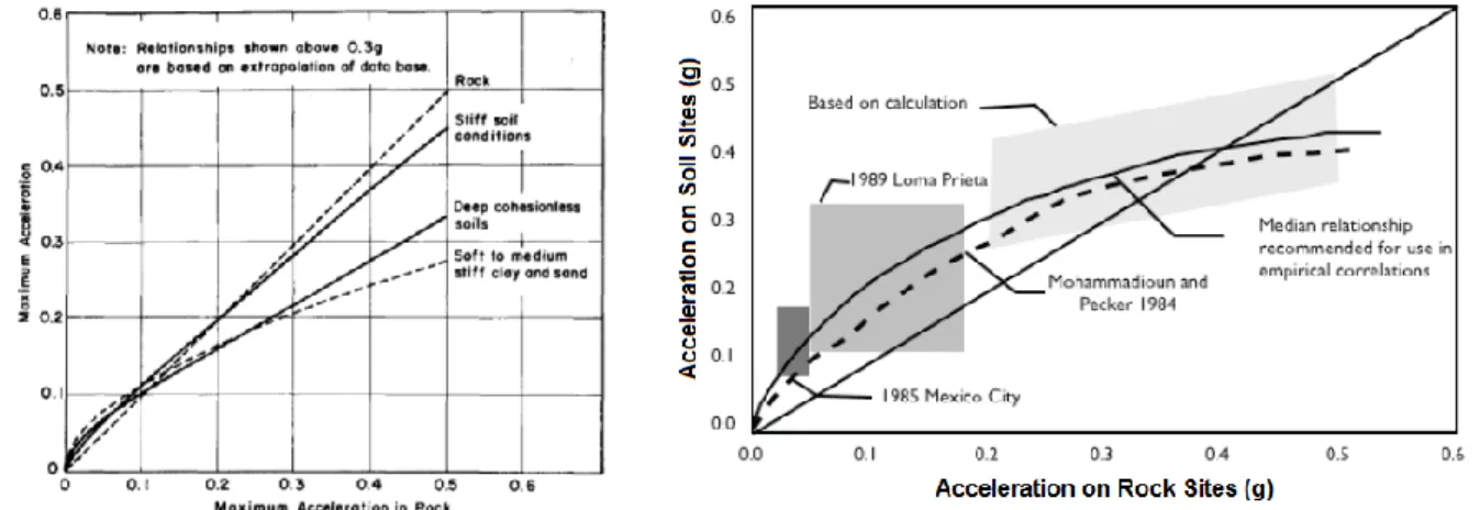
An example is the famous case of the 1985 Mexico City earthquake (Mw = 8.0) where the ground motion recorded on the sediment area was almost 5 times larger than the one recorded on bedrock area. The amplification of ground motion is caused by the impedance between bedrock and sediments. The same 1985 Mexico City earthquake, together with the 1989 Loma Prieta earthquake are also important of adding empirical data and changing the nonlinear threshold from previously 0.13g (Seed et al., 1976; Fig I.3a) to around 0.4g (Idriss, 1990; Fig I.3b). Such as shown in Fig.I.3, the soil nonlinearity tends to deamplify the ground motion responses on soil sites compared to the rock sites. The importance of site effects have

(14)

been as well observed throughout several other earthquakes, such as the 1994 Northridge earthquake, the 1995 Kobe earthquake, and the 2003 Bam earthquake, where the ground motion recorded in sediments were modified compared to the one in bedrock.

Figure I.3. Comparison between acceleration on soil sites and rock sites. (a). Before (taken from Seed et al., 1976), and (b).After the 1985 Mexico City earthquake (taken from Guéguen, 2009, after Idriss, 1990).

The direct site effects, as well source and path properties have been taken into account in the classic criterion for selecting ground motion models for PSHA, as discussed by Cotton et al. (2006). This criterion, however, only incorporates the linear site properties depending on the

value of average shear wave velocity up to 30m depth (Vs30). It is just only recently that the

importance of soil nonlinearity is considered in the construction of GMPEs (Al Atik and Abrahamson, 2010). In addition to the previous GMPEs criterion selection, Bommer et al. (2010) added the importance of non-linear magnitude-dependence and soil nonlinearity, as

well as site effects models without considering the Vs30. The exclusion of Vs30 is important

since different sites with the same Vs30 may have completely different frequency and energy

content. Nonetheless, Vs30 may be the simplest engineering parameter that can be used for

practical purposes. In this paper they show that very few (only 8 from 150) ground motion models incorporate all the criterion proposed, including for example Abrahamson and Silva (2008), Akkar and Bommer (2010), and Campbell and Bozorgnia (2008). Nevertheless, several nonlinear site amplification models, for example Walling et al. (2008) which based on numerical modeling, and Sandikkaya et al. (2013) based on empirical approach, are still using

(15)

Furthermore, population explosion and concentration is always followed by the growth of infrastructure and building constructions, such as previously projected by Bilham (2009). The common perception of the society is that buildings have always been subjected to earthquakes. This concept is not complete, because when ground motion travels through the soil to the structure, the ground motion will travel through and shake the buildings (giving damage to buildings) and then going back to the soil until its energy is totally absorbed by material damping (Housner, 1957; Jennings and Bielak, 1973). This means that the presence of the structures also modifies ground motion; hence, as construction rate increases, the modification of ground motion becomes more complicated. This coupling between soil and structure, known as Soil-Structure Interaction (SSI), has been studied extensively these past years. In addition to aforementioned works from Housner, and Jennings and Bielak; some other examples include Wong and Trifunac (1975), Şafak (1998a), and Guéguen and Bard (2005).

Coburn and Spence (2002) reported that approximately 75% of casualties related by earthquakes are caused by the buildings collapse. This high contribution makes SSI, which controls the structure and ground motion responses in urban area, an essential issue to better determine those responses. A precise definition of SSI is difficult to provide (Kausel, 2010), because whenever coupling between soil and structure modifies the wave propagation, the SSI exists. It means that SSI covers a broad range of problem covering the wave modification from soil to foundation, from foundation to structure, from structure back to the ground (Soil-Structure-Soil Interaction/ SStSI), as well as multi-soil-structure interactions (or Soil-City Interaction/SCI) a concept proposed by Guéguen (2000). Despite all the studies that have been done on this matter, we are still not able to take into account all the complexity, especially in urban area where SCI occurs, it is still a debate on if these effects are detrimental or beneficial.

Guéguen and Bard (2005) did a thorough study on SSI and SStSI using passive experiments at the Volvi test site (Greece), and reported that the latter is significant, thus cannot be neglected. However, in previously mentioned ground motion models, for example, the site effects has not incorporated the important modification from radiated back wave came from the SStSI. Wirgin and Bard (1996) examined the SCI using a simple numerical model from the 1985 Mexico City earthquake case and show the importance of these buildings effects.

(16)

Most of the researches on this matter have been done using numerical approaches and active experiments. Despite all these studies, the importance of SCI has rarely been taken into account in the site effects study, considering the difficulty to choose the governing parameters. Furthermore, nonlinearity has been a complicating factor that is recently incorporated on the SSI study (Pecker and Chatzigogos, 2010; Pecker et al., 2014). This nonlinear dissipating energy is a non-negligible element that often abandoned in the previous studies.

To sum up, the recent global urbanization trends towards concentrated seismic prone cities will have impacts on the increase of seismic risks, firstly through the increase of seismic exposure and vulnerability due to population and building concentrations, and secondly the modification of seismic risks through presence of sediments and dense structures in the urban environment. Therefore, seismic risk analysis is important to understand and predict ground motion responses, estimate damages, and to be able to reduce and minimize losses through urban design strategies and policies. A comprehensive seismic risk assessment needs to integrate a thorough seismic hazard assessment, and complete seismic vulnerability and exposure assessments.

Objectives of the Study

The final goal of seismic risk study was and will always be the reduction of loss. This loss reduction can be achieved by reducing seismic risks. One key element of this reduction is a better understanding and/or prediction of ground motion (hazard). By predicting the ground motion responses, we would be able to design more resistance structures, hence, reducing damage during earthquakes. Contemplating the vast and complex issues of the seismic hazard analysis, this study will focus only on two urban related seismic hazard problems, which are the soil nonlinearity and the soil-structure interaction. Consequently, this study will not cover the vulnerability and exposure parts, although the intersection with these two elements cannot be avoided.

In addition to the direct site effects, the problem of soil nonlinearity and SSI are the key elements of ground motion characteristics on urban area. These ground motion responses are

(17)

important related to the deformation of the near-surface sediments (where most of sub-surface structures are located) and the surface structure. These problems are interesting as they require the combination of seismology, earthquake engineering, geotechnical (soil dynamics), and structural dynamics understanding.

This dissertation is presented in 5 chapters in addition to the general introduction and conclusion. In Chapter 1, the state of the art approaches used for understanding soil nonlinearity (and site effects in general) and soil-structure interaction (as well as the derivative soil-structure-soil and site-city interaction) will be presented. The context and the importance of the effects, the theoretical background, some definitions, as well as some previous studies on these matters will be detailed to give the necessary foundation to comprehend the perspective of the following chapters. This chapter also gives the notion of the 1D wave propagation as well as the deconvolution method that will be used throughout this study.

In chapter 2 and 3, we focus on the soil nonlinearity problem. Although this problem has been observed by the geotechnical engineering community for decade, it has only been recognized recently by the seismology community after the 1989 Loma Prieta earthquake (Chin and Aki, 1991). Most of the studies on this matter were conducted by laboratory experimentation using disturbed sample and/or by numerical modeling. These approaches do not represent what is actually happening in real in-situ conditions, resulting in discrepancies from these results to in-situ measurements. The best approach by far to study this matter is by using the downhole vertical array. There are, however, very few sites that allow the observation of soil nonlinearity, hence, data is limited. To overcome this difficulty, we use two experimental approaches: the dynamic centrifuge test and in-situ observation.

In chapter 2 we use the dynamic centrifuge test to constrain the nonlinear soil problem. The centrifuge test has interested many researchers for it gives a close representation of the real condition. This advanced experiment is important as a benchmark, since in-situ recorded data related to this study is still very limited. To complete the study, Chapter 3 presents the analyses on in-situ recorded data from The Garner Valley Downhole Array (GVDA) and The Wildlife Liquefaction Array (WLA) data. This study is important as an actualization of what happens in real condition. From these two chapters we attempt to answers several questions

(18)

that remain on this matter, e.g. what parameters can be used as a soil nonlinearity proxy (which would be convenient to incorporate the nonlinear problem into the GMPEs for instance)? Is the dynamic centrifuge test capable of capturing the real condition responses? How are the in-situ responses? Are Idrisss 0.3-0.4 g limit still relevant for the nonlinear response of the soil, and whether nonlinear behavior can occur at a very small strain level? May soil nonlinearity occur only at shallow depth? Is nonlinear anisotropy can be observed in real site, changing the isotropic assumption of the site response? And does soil nonlinearity depend only to the intensity of the excitation?

The last two chapters focus on the Soil-Structure Interaction problem using the same approaches, i.e. the centrifuge test (Chapter 4) and in-situ recorded data (Chapter 5). As with before, interests of these approaches are to observe the real ground motion responses and to analyze the discrepancies between laboratory and in-situ measurement. Considering the lack of well instrumented SSI test sites, the observation of in-situ data allows us to analyze what happened in the real site. The complexity of the SSI problem is to separate the different mechanisms related to the soil, soil-structure coupling, and the structure, which are normally mixed as the system response. Although it has been discussed by Todorovska [2009a, 2009b] in an instrumented building, the complexity of the urban environment might add certain confusion and might not reveal the true response of a soil-structure system. Using nonparametric system identification procedures, we try to untangle these different mechanisms to be able to analyze the importance of each element, including their nonlinear behavior.

In Chapter 4, using centrifuge testing, the importance of SSI from only two excitations levels on different type of building (rigid and flexible) is discussed. The SSI behavior of different type of structures is discussed. The system identification procedures are applied to separate different contributing elements of SSI. The nonlinear SSI is discussed by monitoring changes in the modal parameters. In addition, the presence of more than one structure that represents the Site-City Interaction (SCI) problem will also be discussed. How is the modification due to these structure-soil-structure interactions (StSStI)? And what are the observed phenomena when two structures are presented? Furthermore, this chapter will also discuss the free-field contamination problem from the derived Soil-Structure-Soil Interaction (SStSI) problem. We aim to analyze the governed parameters of this free-field contamination, and how much does

(19)

this contamination take effects from the radiated building. Using the same procedure, Chapter 5 analyzes the importance of SSI from multiple earthquake recordings using the in-situ measurement in one site. The identification of each contribution elements are extracted using the same procedures as in Chapter 4. In both chapters, the importance of nonlinearity on SSI is discussed. How far does nonlinearity change the soil-structure system response? And where does this nonlinearity come from? Moreover which elements are influencing these different nonlinearities?

(20)

Chapter 1

From Near Surface Effects to Soil-Structure

Interactions: a 1D Wave Propagation Approach

Variability of ground motion depends on the source (location, focal mechanism, rupture mechanism, and in certain case the directivity effects which are direction dependence), the crustal propagation (waves scattering and attenuation), and the site effects. While the first two effects are mostly of interest to the seismology community, the site effects are of interest to both seismology and engineering communities.

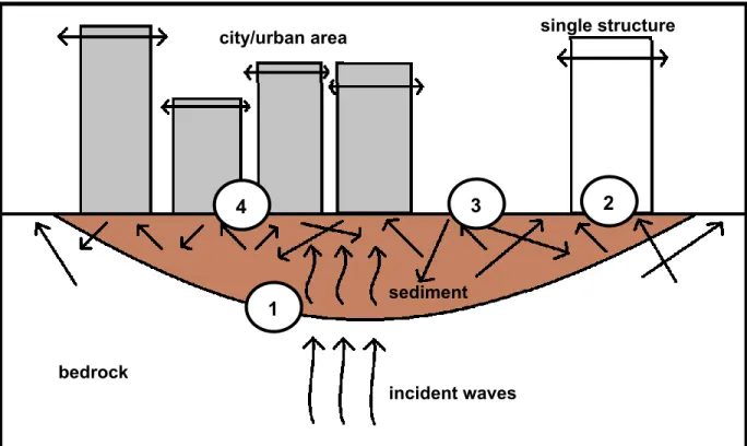
Figure 1.1. Ground motion modification at near surface of an urban area bedrock

incident waves

1

4 3 2

sediment

(21)

Figure 1.1 describes what happens at near surface of an urban area during an earthquake. The waves propagate from the source through a medium. Ground motion characteristics are modified due to the intrinsic properties of the path. Upon its arrival at the bedrock-sediment boundary, the site effects first take place and modify the ground motion. Then, when the waves arrive at the soil-structure interface, the soil-structure coupling effects take place and again modify the waves. Referring to the numbers in Figure 1.1, and after Guéguen (2000) these effects consist of Site Effects (No.1), Soil-Structure Interaction/SSI (No.2) that modifies the response of the structure due to the coupling between soil and structure, Soil-Structure-Soil Interaction/SStSI (No.3) that corresponds to the inertial damping due to the energy of vibration radiated back into the soil through surface seismic waves, and Site-City Interaction/SCI (No. 4) when the urban medium is composed by several buildings. When there are only 2 buildings, the effects are called Structure-Soil-Structure Interaction/StSStI. This means that the seismic responses of soil-structure system in the urban area are primarily governed by two effects: site effects and soil-structure interaction. It is therefore essential to study and characterize these phenomena to be able to incorporate them into the seismic risk analysis, to further be applied in building codes, urban planning, insurance calculations, as well as emergency and/or mitigation planning.

Site effects and soil-structure interaction effects have been studied and discussed as the fundamental elements of seismic risk management. In most of the literature, the discussions of these effects are inseparable, for example in Kramer (1996), Oliveira et al. (2006), and Schanz and Iankov (2009). Site effects or near surface effects are the effects caused by a local geology configuration (also known as local geology effects). These site effects can be distinguished as direct site effects, induced site effects, and geometry effects. Although there exists other site effects such as the topography effects (when the waves propagate into a convex area, e.g. mountain summit) and surface ruptures effects, they appears locally and will not be discussed further.

Direct site/sediment effects (classic site effects) happen due to the impedance between bedrock (stiff soil) and sediment (soft soil). These effects are manifested through ground motion amplification. Direct sediment effects have been studied comprehensively especially after the 1985 Mexico earthquake (Campillo et al., 1989; Chavez-Garcia and Bard, 1994).

(22)

Introduction | 13

These effects, however, will not be of interest in this study. Induced site effects are in most cases demonstrated as soil nonlinearity. Soil nonlinearity is an intrinsic problem of the soil, i.e., how soil is deformed when subjected to different levels of earthquake stress. These effects are manifested through a ground motion deamplification and a shear wave velocity reduction. Depending on different parameters, these effects can be followed by either the liquefaction phenomenon, cyclic mobility phenomenon, or the slope instabilities. The detail of this effect is discussed in Chapter 1.1.

Geometry effects, also known as basin effects, are those induced by the geometry or the presence of the sedimentary basin. These effects consist of the trapping and the resonance of the waves inside the basin, considered 2D and 3D. Some studies have incorporated the basin effects, such as Frankel et al. (2002) in the Seattle basin using seismic recordings from the M 6.8 Nisqually earthquake, Cornou et al. (2004) in Grenoble basin where the noise energy bursts and trapping of harmonic waves were observed, Sleep (2010) who indicated a reverberation of surface waves within sedimentary basins, and Gélis and Bonilla (2012) where the 2D basin effects were taken into account in numerical modeling. These effects, however, will not be of interest in this study.

The first two aforementioned effects (direct effects and soil nonlinearity) are those that occur most frequently in an urban area due to soft sediment deposits. These near surface effects are complicated due to their contradictory effects of amplification and deamplification of the ground motion. Since both effects appear normally during strong earthquake excitation, these effects are mixed and their separation is rarely examined.

In the presence of a stand-alone structure, there is a coupling between the soil and structure when seismic waves travel from sediment to the structure that modifies the ground motion characteristics. These interactions, known as SSI, consist of the kinematic interactions and inertia interactions. Kinematic interactions include the scattering phenomenon due to the dynamic impedance between soil and structure, where structure is normally represented by the foundation. Inertia interactions come from the vibration of the structure system that depends on the dynamic properties of the structure. The kinematic effects are present at lower level of ground shaking by the long period and radiation damping. At stronger ground motion level, the inertial interactions become more dominant, shown by displacements and bending

(23)

strains concentrated near the ground surface. The detail of this effect is discussed in Chapter 1.2.

After this modification, the structure vibrates and radiates back-waves to the free-field. These back-waves join the incident field waves and hence modify their properties. This free-field modification is known as the Soil-Structure-Soil Interaction (SStSI). In a city or an urban area where more than one structures are present, the waves propagate and are modified from one structure to another depending on the modification of their properties. These interactions are very complex depending, for example, on the structure or the density of the city (Guéguen et al., 2002).

1.1. Soil Nonlinearity

1.1.1. Rheological Notions

Unlike the direct site effects that are engendered by the impedance of the materials, soil nonlinearity effects are generated by intrinsic properties of the material, in this case the sediment/soil. These intrinsic properties control the responses of the soil when subjected to dynamic loading. Before moving further, it is important to review the rheological problem of the soils during cyclic loading (earthquake).

Like other materials, soil responses depend on its stress-strain evolution. The stress states at different points in a soil mass are characterized by the normal (σ) and shear (τ) stresses. Equation 1.1 shows the stress description in a matrix form, where x, y, and z indicate the

directions, so that σxx, σyy, and τxy are the normal stresses and the shear stress that are working

on the xy-plane.

� � �

�

_��

�

_��

�

_��

�

_��

�

_��

�

_��

(24)

Soil Nonlinearity | 15

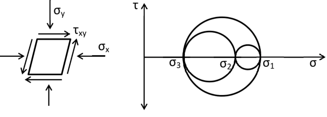
Since soils do not resist tensile, the stress terms are associated to normal compressive stress and shear stress that are present during seismic loading. The stress state of any points in a soil mass can be represented by a Mohr circle representation as shown in Figure. 1.2.

Figure 1.2. Stress state and its Mohr circle representation at any points in a soil mass under earthquake excitation

σ1 is the largest principal stress, called major principal stress, σ3 is the smallest principal

stress, called minor principal stress, and σ2 is the intermediate principal stress. On the xy-plane

(Figure. 1.2 left), σyy is the major principal stress, and σxx is the minor principal stress.

Rheological problem of soils have been based mainly on laboratory experiment, especially from triaxial compression tests. Based on these observed experiments, different constitutive models were determined to explain behavior of soils for different stress conditions. Fundamental definitions of some soil conditions under cyclic loading are discussed below.

 Linear x Nonlinear

At small strain, soil behavior follows the Hookes law where force (stress) is proportional to deformation (strain). � � � ∙ � (1.2) � � � ∙ � (1.3)

σ

y

σ

x

τ

xy

σ

3

σ

2

σ

1

σ

τ

(25)

In Equations (1.2) and (1.3), E is the Youngs modulus, ε is the normal strain, G is the shear modulus, and γ is the shear strain. In tensorial, Equation 1.2 can be written as:

�� _{∶ ��}�_(1.4)

where C is the stiffness in 4th order tensor, and e indicates the elastic state. The stiffness

tensor, C, depends on the Lame coefficients λ and μ:

� � �Ι⨂Ι � 2�| (1.5) where I is the second-rank identity tensor and | is the symmetric part of the fourth-rank identity tensor. The Lame coefficients depend on Youngs modulus, E, and a poisson coefficient, ν.

� � ��

�1 � ��1 � 2�� (1.6�

� � �

2�1 � �� (1.7)

As we can see in Figure 1.3, linear behavior always occurs in the elastic region (Line A-B). Nonlinear behavior on the other hand, occurs when the stress and strain value no longer follows a proportional (linear) relationship. Nonlinear behavior can occur in the elastic region (Line B-C) as well as in the plastic region (Line C-D).

Figure 1.3. Stress-strain relationship model in materials.

stre

ss,

σ

(26)

 Elastic x Plastic

Soils are said to be in an elastic state if after being deformed, they return to their original state. On the other hand, soils are said to be in a plastic/inelastic state if after having been deformed they end up having some permanent deformations (Figure 1.3).

 Isotropic x Anisotropic

Soils are said to be isotropic if they have uniformity in all directions. However, in most cases, soils are anisotropic, thus they do not deform uniformly in all directions. Nonetheless, in most simplified models, the isotropic model is used and its elastic relation can be described as:

� � � � � � �_�� _�� _�� _��_{� �}� � � � � � � � �1 � ��1 � 2�� 1 � � � � 0 0 0 � 1 � � � 0 0 0 � � 1 � � 0 0 0 0 0 0 1 � 2� 2⁄ 0 0 0 0 0 0 1 � 2� 2⁄ 0 0 0 0 0 0 1 � 2� 2⁄ �� _�� _�� _�� _��_{� �}� � � � � � (1.8) These rheological notions are important because variations of ground motion are controlled by the nonlinear responses of the soil. These soil dynamic behaviors depend on the characteristics of the soils and the incident waves which control the frequency-dependent soil dynamic parameters, i.e., the shear modulus (since earthquake controls the shear properties of the soil) and the damping (ξ). Under a strong level of shaking, the induced deformation will exceed the linear limit. In addition, when strain increases, the shear modulus decreases as the material damping increases. An increase of material damping results in a deamplification of ground motion acceleration, and since shear wave velocity (Vs) is related to G and mass density (ρ) as according to

�� /� (1.9) , the shear wave velocity decreases when strain increases.

(27)

1.1.2. Existing Methods and Studies

Several approaches exist to study the dynamic responses (shear modulus, shear wave velocity, and material damping) of soils under cyclic loading. These approaches are based on theoretical, numerical, or experimental approaches. Experimental approaches can be categorized into two categories: laboratory experimentations and field tests.

Due to the use of a discrete sample, laboratory tests do not represent real soil conditions. Nevertheless, their preliminary results are important as a benchmark or reference for further studies. Most laboratory experiments are conducted to determine the behavior of soils and are done on cohesionless soils that lack cohesion. There are two reasons to this: first, because the evolution from linear to nonlinear behavior was observed to occur more in this type of soils, and second, because most laboratory experiments are more adapted to this type of soils. Some early studies are presented by Seed and Idriss [1969, 1970], and Hardin and Drnevich (1970) where the governing parameters for G and ξ are the shear strain (γ), effective mean principal

stress (σm), void ratio (e), loading cycles (N), and degree of saturation (S). Seed et al. (1984)

discussed the moduli and damping factors for dynamic analyses of cohesionless soils using the cyclic undrained triaxial tests. Vucetic and Dobry (1991) studied the effect of plasticity index (PI) during cyclic response on laboratory testing using different over consolidated ratio (OCR). As laboratory equipments advance, new techniques are developed. Some existing laboratory measurements include the cyclic triaxial test (e.g. Boulanger et al., 1998), resonant column test, bender element test (e.g. Atkinson, 2000), direct simple shear test, and cyclic torsional shear test (e.g. Georgiannou et al., 2008).

Based on these dynamic properties measurements, some thresholds of cohesionless soil nonlinearity were established. These thresholds are related to linear-equivalent analyses because linear-equivalent models are still the most preferred approach to analyze the nonlinear problem. Figure 1.4 shows the popular shear degradation modulus and an increase in the damping curve as a function of shear strain.

(28)

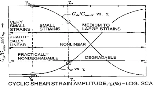
Figure 1.4. Typical shear degradation modulus and damping curves in function of shear strain (after Vucetic, 1994).

In this figure, Vucetic (1994) separated two different thresholds for nonlinear analyses, i.e.

1. γtl which is the linear cyclic threshold shear strain, and

2. γtv which is the volumetric cyclic threshold shear strain.

From these two limits we can characterize the behavior of the soils. Therefore:

1. when γ < γtl, the soils exhibit a linear-elastic behavior.

2. when γtl < γ < γtv, the soils are in nonlinear-elastic zone. This means that nonlinear

behavior already occurs, but they remain elastic with negligible or no permanent deformation.

3. when γ > γtv, the soils are in a nonlinear-plastic zone, where soils behave

nonlinearly and permanent deformations can no longer be neglected.

Hardin and Black (1968), Drnevich and Richart (1970), and Anderson and Richart (1976) set

the volumetric threshold, γtv to 10-4. Other laboratory experiments were done in a drained

condition, where water can flow freely. Vucetic (1994), and Youd (1972) found the γtv(Dr) at

a strain value of 2x10-4. In an undrained condition, where there is no volumetric change,

Dobry and Ladd (1980) set the volumetric limit γtv to 10-4, and Johnson and Jia (2005) saw

that nonlinear elastic started to occur at a strain value of10-7.

In addition to these tests, there exist some laboratory scaled model techniques, such as shaking tables and centrifuge tests that have been used to extract the dynamic properties of

(29)

soils. Some examples can be found in Brennan et al. (2005) and Li et al. (2013) where shear stresses and shear strains are calculated indirectly using the accelerometers measurements, following Equations (1.10)-(1.11). τ�� (1.10) �_�� 1.11�

Here, z is the depth, ü is the acceleration, and u is the displacement.

Measurement of dynamic soil properties can also be done using field experiments as characterization tests. This can be divided to invasive and non-invasive methods. Standard tests based on non-invasive field measurements include the seismic refraction test, seismic reflection test, and spectral analysis of surface waves test (SASW). The invasive methods include the seismic cross-hole test, seismic downhole test, standard penetration test (SPT), and cone penetration test (CPT). Most of these tools are active measurements, which means that the measurements are done by introducing an active source. In geotechnical measurements such as SPT and CPT, empirical equations exist between the geotechnical results and shear wave velocity values such as described in Wair et al. (2012). Further details for both laboratory and field experiments can be found in any geotechnical reference textbooks, e.g. Kramer (1996).

Numerical approaches have been developed to characterize the cyclic soil behavior. The simplest numerical approach that has been used widely is the linear equivalent model. This approach uses an idealization of nonlinear problem by treating them as an equivalent-linear model, and finding the generalized evolution of shear modulus and damping. Although simple, this approach is less realistic compare to other numerical methods. More accurate approaches can be found for example by the cyclic nonlinear models where the actual stress-stain paths are observed during a cyclic loading. This loading and unloading are characterized using some additional constraints, for example the extended Masing rules. However, these models are not able to take into account the shear-induced volumetric strain. The most complex and realistic numerical approaches are the theoretical constitutive models. These

(30)

models describe the evolution from linear elastic to soil plastic condition up to rupture. We can refer to the fundamental Mohr-Coulomb model which takes into account the elastic-perfectly plastic model for isotropic material. We can also refer to Drucker-Prager model, Tresca, Von-Mises, and Hill, which can be applied for both isotropic and anisotropic materials. Most of these constitutive models take into account only a compression limit state and can be coupled with any tensile criterion for complete assessments, although it may or may not be necessary considering that soils do not resist tensile. We do not discuss the details of these models, and the readers can be referred to any rheological textbooks (e.g. Yamamuro and Kaliakin, 2005). These models are elastic-perfectly plastic models, and so can be completed by integrating the strain hardening properties of the soils to models such as the Cam-Clay or Modified Cam-Clay models that were developed at Cambridge University (Roscoe and Burland, 1968; Roscoe, 1970), and the Hujeux model developed at Ecole Centrale Paris (Hujeux, 1985). The latter are the most used constitutive models at the present time.

Although the problem of soil nonlinearity had been recognized by the earthquake engineering community, it was not after the 1989 Loma Prieta earthquake that seismologists acknowledged this problem (Chin and Aki, 1991; Aki, 1993). At the beginning of the observations, the nonlinear footprints can be identified by a deamplification of ground motion, a shear wave velocity reduction, and a shift in energy towards a lower frequency (as shown by the linear-equivalent modeling). Yu et al. (1992) analyzed the nonlinear response of several strong motion recordings using numerical codes. They concluded that during nonlinear responses, there is a frequency dependency of the shifting of Fourier spectral ratios, which are unaffected at low frequency, decreasing at moderate frequency and increasing at high frequency. These results showed that nonlinear behavior of the soils is governed not only by the amplitude of ground motion but also its frequency content. Beresnev and Wen (1996) wrote a short review on soil nonlinearity from a seismologist point of view. Şafak (2001), and Trifunac (2009) examined the local site effects by taking into account both amplification due to different impedance and nonlinear site responses. An empirical nonlinear curve was established by Idriss (1990) adding the data observations from the Mexico City and Loma Prieta earthquake (Figure I.3) where the nonlinear behavior, marked with the deamplification of ground motion, starts at around 0.3 to 0.4 g (of ground motion recorded at rock sites).

(31)

Following the Loma Prieta earthquake, multiple site nonlinearity observations have been studied for different earthquake events. Due to its simplicity, most processing are done using linear-equivalent models such as shown in the following examples, unless otherwise stated. These observations of site nonlinearity can be done using borehole or surface recordings depending on the availability of the seismic array at site. Some observations based on borehole observations were done by Satoh et al. (1995) who examined the recordings at the Ashigara Valley from four earthquake recordings during the period of 1990 and 1991. Using the inversion technique, the nonlinear actions were observed by a 10% Vs reduction and a 50% increased damping. Sato et al. (1996), Aguirre and Irikura (1997), and Satoh et al. (2001) used the recordings at different areas that were struck by the 1995 Kobe earthquake. Applying spectral analysis and inversion techniques, Vs reductions were observed and strain-dependent nonlinear characteristics were formed. Pavlenko and Irikura [2002, 2003] also used the recordings and analyzed the time-dependent model for nonlinear behaviors at these sites, following the changes of stress-strain curve in the time domain. Nonlinearity evidences were also present at the 1994 Northridge earthquake. Bonilla et al. [2003, 2005] worked with borehole data in Japan and California and modelled the shear modulus degradation due to nonlinearity; Assimaki et al. (2008a) showed the nonlinear effects during the 2003 Miyagi-Oki earthquake using different techniques of surface-to-downhole spectral ratios (SSR), cross-spectral ratios, and horizontal-to-vertical (H/V site) responses. Although these observations are mostly found at sediment sites, Régnier et al. (2013) recently showed some nonlinear behavior in relatively stiff soil during moderate earthquakes from the Japanese KiK-net strong motion data using the SSR techniques.

When borehole data recordings do not exist, nonlinear observations are obtained from the available surface recordings, mostly by comparing the rock and soil sites that are situated in the vicinity. As discussed in Steidl et al. (1996), however, the difficulty of choosing the reference rock sites may results in a misleading conclusion. Field et al. (1997) compiled multiple surface recordings at sediments and hard rock from the 1994 Northridge earthquake, and showed a ground motion deamplification during strong motion at sediments. Hartzell (1998), and Beresnev et al. (1998) did a similar analysis by comparing the weak and strong ground motion and they found a deamplification due to strong ground motion around the San Fransisco and Los Angeles basin. Dimitriu et al. (2001) investigated the dependence of high

(32)

nonlinearity using accelerograms from Lefkas, western Greece. Frankel et al. (2002) observed a shift of resonance frequency towards lower frequency and studied the basin effects in Seattle for the 2001 Nisqually earthquake. Moreover, Rubenstein and Beroza [2004, 2005] and Rubenstein et al. (2007) showed evidences of nonlinearity from different earthquakes, i.e., the 1989 Loma Prieta earthquake, the 2003 Tokachi-Oki earthquake, and the 2004 Parkfield earthquake. Using a waveform cross correlation, they identified velocity reduction in shallow sediments, but not significant at greater depth.

In addition to these observations, some numerical studies were conducted in order to be able to predict the nonlinear soil effects. This kind of prediction is normally done by developing mathematical models for specific soil types, sites, and earthquakes, and then comparing the results with responses from seismic recordings. Hartzell et al. (2004) used different approaches ranging from equivalent-linear to nonlinear models and gave recommendations for formulations of the nonlinearity. They showed that their model is comparable to the 2001 Nisqually earthquake for class D and E sites. Pavlenko (2001) used a nonlinear system identification method to study the evolutions of the nonlinear effects in frequency domain. Bernardie et al. (2006) implemented CyberQuake constitutive models that were derived from the Hujeuxs model to simulate the nonlinear site response during the 1999 Chi-Chi earthquake.

In spite of all these extensive researches, the review from Field et al. (1998) summed up the remaining challenges from a nonlinearity study that share the same perspectives in the context of this study. First, even though laboratory studies do not reflect the in-situ behavior of soils, they are important to have as a reference. These studies however have to be completed with in-situ data. The best approach by far to study this matter is by using the downhole vertical array. Unfortunately, this downhole array data are very limited. In terms of processing approaches, while equivalent-linear model is very limited to explain the nonlinear behavior (compare to complex constitutive models, for instance), its simplicity regarding to the extensive results that can be provided will still be the first choice for researchers to conduct nonlinear studies. In addition, we notice that most early studies based on laboratory experiments captured only the nonlinear-plastic limit (since plastic deformation starts to occur after passing this threshold), ignoring the nonlinear elastic response that occurs at very small strain value.

(33)

1.2. Soil-Structure Interaction (SSI)

Soil-Structure Interaction has received increased attention, even more than Soil Nonlinearity. While the fundamental tools to treat this problem have been extensively discussed, some crucial problems related to SSI remain unsolved. Kausel (2010) conducted a complete and thorough investigation of the early history of soil-structure interaction. The author agrees on Kausels definition on soil-structure interaction: it is eminently clear that the concept of soil-structure interaction refers to static and dynamic phenomena mediated by a compliant soil and a stiffer super-structure, but the discipline encompasses so many different, sometimes tenuously connected aspects that is difficult indeed to enounce a cogent definition in just a few words. In his paper, Kausel mentioned that the study of SSI began in the nineteenth century with the development of some solid mechanics fundamental solutions, for example by Lamé and Clapeyron with the development of half-space problems. Another milestone came from Stokes solutions which later became the fundamental of Boundary Element Method (BEM), geophysics, acoustics, and other branches of science. In addition, Boussinesq developed solutions for more complicated problems, especially in static SSI problems. However, it was not until 1936 that Reissner started the study on the dynamic SSI where time-harmonic vertical loads were applied to circular disks on elastic half-spaces.

1.2.1. Dynamic Equilibrium of the Structures

The problems of structural dynamics have been of interest not only to the civil engineering community, but also the seismologist community. These problems have been discussed in details in many structural dynamics textbooks, such as in Chopra (2007). A fixed-base structure is characterized by its degrees of freedom (DOF) which are the number of relative displaced positions of all the masses in the system. Structures in SSI system can be simplified as a single degree of freedom (SDOF) system that consists of a concentrated/ lumped mass, m, at the roof level contributing to the inertial properties of the system, the stiffness of the system, k, that is modeled by a massless frame, and a viscous damper (a dashpot), c, that dissipates vibrational energy of the system. The dynamics of this system are characterized by the following three forces that are associated to the aforementioned elements and the displacement, u(t) at any DOF point, respectively: the inertial forces acting on the mass at one

(34)

Soil-Structure Interaction (SSI) | 25

instant time (�_� � �. ��), the elastic resisting forces, associated with the rigidity of the

structure (�� . �), and the damping resisting forces due to a linear viscous damper

�� . ��.

The equation of motion for elastic SDOF systems under an earthquake excitation can be derived by applying either the DAlemberts principle or Newtons second law of motion to the equations, yielding:

�. ��_{� �. �� . � � 0}

�. �� _�� . �� . � � 0

�. �� . �� . �� . 1�_{. ��}

�� (1.12)

where üt is the total acceleration and üg is the ground motion acceleration. The solution to

Equation 1.12 can be found in many references, for example in Chopra (2007). Under earthquake excitations, the system can be modeled as in Figure 1.5.

Figure 1.5. SDOF system under harmonic excitation (modified after Guéguen, 2000)

1.2.2. Kinematic and Inertial Interactions

Soil-structure interaction phenomena can be divided to two different interactions. Based on their order of appearances, these interactions are summarized as follows:

ut_(t)

u(t)

(35)

1. Kinematic Interaction

After modifications due to the site effects (including nonlinearity), seismic waves go through another modification caused by an impedance between soil and structure (represented by its foundation), which occurs at the soil-structure interface. The different impedances between the rigid foundation and soft soils cause the incident waves to be diffracted back to the ground and transmitted to the structure. Transmitted waves that are the Foundation Input Motion (FIM) are different than the incident motion. The scattering of this incident waves depends on the foundation stiffness, surface and geometry of the foundations, and the embedment type. In this study we are not interested to go into details on this kinematic interaction. More coherence studies on the impedance functions and dynamic soil-foundation interaction can be found in Gazetas (1991), Gazetas and Makris (1991), and Makris and Gazetas (1992). Lai and Martinelli (2013) noticed that in the special case of a shallow foundation struck by a vertically propagating S-wave, the kinematic interaction is not present.

2. Inertial Interaction

The inertial interaction is caused by the transmitted waves that travel and vibrate structure due to the material damping and stiffness modification. This interaction also includes the impedances between foundation and structure that have to be included in an inertial interaction through the foundation impedance matrix. In addition, similar to what happens inside the soils under a strong excitation, building must behave nonlinearly. This behavior is

frequency dependent, referring to Equation 1.13, where Tn is the natural period of the

structure.

�� 2��

�

� �1.13�

1.2.3. Existing Methods

Similar to other researches, there exist three main axes of methods to study the problem of soil-structure interaction, i.e., the Theoretical, Numerical and Experimental methods. The theoretical methods might be the oldest approaches that have been explored by researchers. These methods attempt to provide a closed-form solution to the equation of motion of the systems. We can refer to the previously mentioned Kausels (2010) paper that provides the

(36)

historical development of these theoretical methods. Early works that covered the whole dynamic of building-soil interaction can be found for example in Jennings and Bielak (1973) who applied the discrete foundation and half-space analyses to an idealized structure. However, in this dissertation we will not provide any further details except when it is necessary.

The numerical methods can be distinguished to two different approaches (Pecker, 2007, and Lai and Martinelli, 2013):

1. Direct/Global Method

This method consists of solving one global dynamic equation (Equation 1.12) that takes into account both the soil and structure systems using any discretization techniques, e.g. Finite Element Method (FEM), Spectral Element Method (SEM), and Finite Difference Method (FDM). Although its solution is direct and adaptable for either a linear or a nonlinear analysis, the global method is arduous and expensive in terms of computation. The results depend on the constitutive law that is adapted for the soil and structure systems, and comprehensive and thorough investigations of the geotechnical condition are necessary in order to produce relevant results. This direct method is preferred when a detailed analyses is needed, for example for historical monuments. However, for urban modeling, this method will not be efficient regarding its computational time and cost.

2. Indirect/Substructure Method

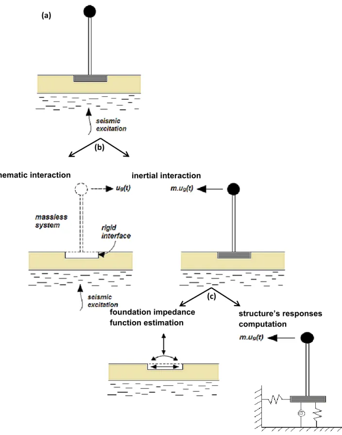
Rather than solving the SSI problem as one global system as in the direct method, the indirect/substructure method decomposes the SSI problem into sub-systems in order to separate the effects of kinematic and inertia interactions. The response of each sub-system is solved individually and step-by-step successively. Since each sub-system is solved separately, this method is less arduous than the direct method and is a preferred solution to urban assessment when a scale of a city is analyzed. The classic decomposition of the SSI system for the substructure method that has been widely used (e.g. Kausel et al., 1976; Endres et al., 1984; Guéguen, 2000; Mylonakis et al., 2006; Pecker, 2007; and Lai and Martinelli, 2013) is shown in Figure 1.6. For each sub-system, we need to formulate the equation of motion including the boundary conditions (the stress and displacement continuity) at each interface. These equations are preferred to be solved in frequency domain.

(37)

This decomposition consists on solving these following three steps:

 Determination of rigid foundation movement due to the kinematic interaction.

The Foundation Input Motion (FIM) is determined at this step. The equation of motion of sol-foundation sub-system (without structure) is:

��_�� 0 0 �� _�∗ ��_�∗� � � �_�� _�� _�� _�� _�∗ ��_�∗� � � 0 �_�� 1.14�

Here, m is the mass, K is the stiffness, F indicates foundation, S indicates soil, FS indicates a foundation-soil system, ~ indicates the frequency domain, R is the model

boundary, and thus the vector QR does not have any zero values except at these

nodes. The underline denotes a vector as two underlines denotes a matrix, u* is the

displacement of the kinematic interaction, and ui is the displacement of the inertial

interaction, where

�� _{� � � �}∗_�1.15�

 Estimation of foundation impedance matrix, done by solving the equation of

motion as follows: ��_�� 0 0 �� _�� _�� _�� _�� _�� _�� _�� _�� 0 � �1.16�

where PF indicates the force that is working on the foundation.

 Computation of the response of the structure related to the previously solved

impedance matrix and the kinematic interaction. This is done by solving the equation of motion as follows: ��_�� 0 0 ��_� �� _�� _�� _�� _� �� _�� 0 ��_�� ∗� �1.17�

(38)

Figure 1.6. (a) The geometry of soil-structure interaction problem; (b) decomposition of ISS into kinematic and inertial interaction; (c) decomposition of inertial interaction into estimation of foundation impedance function and structure system response. (modified after Guéguen, 2000; Mylonakis et al., 2006)

kinematic interaction inertial interaction

foundation impedance

function estimation structures responses _computation

(a)

(c) (b)

(39)

Here, B indicates the building, � is the transformation matrix, �� is the displacement vector and rotation of the center of the foundation, with

��_� � � ��_� �1.18�

and ��_� is the impedance matrix of the foundation.

In addition to these methods, there exists a macro-element method that is considered to be effective to treat the nonlinear problem of the whole SSI system that is not taken into account by the sub-structure method.

A simple analogic model related to separation of different motions when SSI takes place during earthquake can be seen in Figure 1.7. (Guéguen, 2000; Pecker, 2007).

Figure 1.7. Model of the soil-foundation-structure with its related motion (taken from Guéguen, 2000)

In Figure 1.7, h and r denote horizontal and rotation, respectively, and 0 and 1 indicate the position of foundation (bottom) and top of the structure, respectively. These motions are:

1. Translation of the soil due to the ground motion, ug,