Estimation of observation errors for large-scale atmospheric inversion of CO 2 emissions from fossil fuel combustion

HAL Id: hal-02903707

https://hal.archives-ouvertes.fr/hal-02903707

Submitted on 29 Oct 2020

HAL is a multi-disciplinary open access

archive for the deposit and dissemination of

sci-entific research documents, whether they are

pub-lished or not. The documents may come from

teaching and research institutions in France or

abroad, or from public or private research centers.

L’archive ouverte pluridisciplinaire HAL, est

destinée au dépôt et à la diffusion de documents

scientifiques de niveau recherche, publiés ou non,

émanant des établissements d’enseignement et de

recherche français ou étrangers, des laboratoires

publics ou privés.

atmospheric inversion of CO 2 emissions from fossil fuel

combustion

Yilong Wang, Grégoire Broquet, Philippe Ciais, Frédéric Chevallier, Felix

Vogel, Nikolay Kadygrov, Lin Wu, Yi Yin, Rong Wang, Shu Tao

To cite this version:

Yilong Wang, Grégoire Broquet, Philippe Ciais, Frédéric Chevallier, Felix Vogel, et al.. Estimation

of observation errors for large-scale atmospheric inversion of CO 2 emissions from fossil fuel

combus-tion. Tellus B - Chemical and Physical Meteorology, Taylor & Francis, 2017, 69 (1), pp.1325723.

�10.1080/16000889.2017.1325723�. �hal-02903707�

Full Terms & Conditions of access and use can be found at

https://www.tandfonline.com/action/journalInformation?journalCode=zelb20 ISSN: (Print) 1600-0889 (Online) Journal homepage: https://www.tandfonline.com/loi/zelb20

Estimation of observation errors for large-scale

atmospheric inversion of CO

₂

emissions from fossil

fuel combustion

Yilong Wang, Grégoire Broquet, Philippe Ciais, Frédéric Chevallier, Felix

Vogel, Nikolay Kadygrov, Lin Wu, Yi Yin, Rong Wang & Shu Tao

To cite this article:

Yilong Wang, Grégoire Broquet, Philippe Ciais, Frédéric Chevallier, Felix

Vogel, Nikolay Kadygrov, Lin Wu, Yi Yin, Rong Wang & Shu Tao (2017) Estimation of observation

errors for large-scale atmospheric inversion of CO

emissions from fossil fuel combustion, Tellus B:

Chemical and Physical Meteorology, 69:1, 1325723, DOI: 10.1080/16000889.2017.1325723

To link to this article: https://doi.org/10.1080/16000889.2017.1325723

© 2017 The Author(s). Published by Informa UK Limited, trading as Taylor & Francis Group

Published online: 16 May 2017.

Submit your article to this journal Article views: 2003

View related articles View Crossmark data

Tellus

PUBLISHED BY THE INTERNATIONAL METEOROLOGICAL INSTITUTE IN STOCKHOLM

Estimation of observation errors for large-scale

atmospheric inversion of CO

₂

emissions from fossil fuel

combustion

By

YILONG WANG

_{, GRÉGOIRE BROQUET}

_{, PHILIPPE CIAIS}

_{, FRÉDÉRIC CHEVALLIER}

_,

FELIX VOGEL

_{, NIKOLAY KADYGROV}

_{, LIN WU}

_{, YI YIN}

_{, RONG WANG}

_and

SHU TAO

_,

_{Laboratoire des Sciences du Climat et de l’Environnement, CEA-CNRS-UVSQ- Université Paris}

Saclay, Gif-sur-Yvette Cedex, France;

_{Laboratory for Earth Surface Processes, College of Urban and Environmental}

Sciences, Peking University, Beijing, China

(Manuscript received 22 December 2016; in final form 27 April 2017)

ABSTRACT

National annual inventories of CO₂ emitted during fossil fuel consumption (FFCO₂) bear 5–10% uncertainties for developed countries, and are likely higher at intra annual scales or for developing countries. Given the current international efforts of mitigating actions, there is a need for independent verifications of these inventories. Atmospheric inversion assimilating atmospheric gradients of CO₂ and radiocarbon measurements could provide an independent way of monitoring FFCO₂ emissions. A strategy would be to deploy such measurements over continental scale networks and to conduct continental to global scale atmospheric inversions targeting the national and one-month scale budgets of the emissions. Uncertainties in the high-resolution distribution of the emissions could limit the skill for such a large-scale inversion framework. This study assesses the impact of such uncertainties on the potential for monitoring the emissions at large scale. In practice, it is more specifically dedicated to the derivation, typical quantification and analysis of critical sources of errors that affect the inversion of FFCO₂ emissions when solving for them at a relatively coarse resolution with a coarse grid transport model. These errors include those due to the mismatch between the resolution of the transport model and the spatial variability of the actual fluxes and concentrations (i.e. the representation errors) and those due to the uncertainties in the spatial and temporal distribution of emissions at the transport model resolution when solving for the emissions at large scale (i.e. the aggregation errors). We show that the aggregation errors characterize the impact of the corresponding uncertainties on the potential for monitoring the emissions at large scale, even if solving for them at the transport model resolution. We propose a practical method to quantify these sources of errors, and compare them with the precision of FFCO₂ measurements (i.e. the measurement

errors) and the errors in the modelling of atmospheric transport (i.e. the transport errors). The results show that both the representation and measurement errors can be much larger than the aggregation errors. The magnitude of representation and aggregation errors is sensitive to sampling heights and temporal sampling integration time. The combination of these errors can reach up to about 50% of the typical signals, i.e. the atmospheric large-scale mean afternoon FFCO₂ gradients between sites being assimilated by the inversion system. These errors have large temporal auto-correlation scales, but short spatial correlation scales. This indicates the need for accounting for these temporal auto-correlations in the atmospheric inversions and the need for dense networks to limit the impact of these errors on the inversion of FFCO₂ emissions at large scale. More generally, comparisons of the representation and aggregation errors to the errors in simulated FFCO₂ gradients due to uncertainties in current inventories suggest that the potential of inversions using global coarse-resolution models (with typical horizontal resolution of a couple of degrees) to retrieve FFCO₂ emissions at sub-continental scale could be limited, and that meso-scale models with smaller representation errors would effectively increase the potential of inversions to constrain FFCO₂ emission estimates.

Keywords: fossil fuel, radiocarbon, global atmospheric inversion, observation error, Europe

Tellus B: 2017. © 2017 The Author(s). Published by Informa UK Limited, trading as Taylor & Francis Group.

This is an Open Access article distributed under the terms of the Creative Commons Attribution License (http://creativecommons.org/licenses/by/4.0/), which permits unrestricted use, distribution, and reproduction in any medium, provided the original work is properly cited.

Citation: Tellus B: 2017, 69, 1325723, https://doi.org/10.1080/16000889.2017.1325723

1

mismatch due to different spatial representativeness, etc., which are grouped under the generic term observation errors). Atmos-pheric inversions have been used so far for estimating natural CO₂ fluxes, with most studies being at the scale of large regions (Bousquet et al., 2000; Gurney et al., 2002), and few studies at the scale of small regions (Lauvaux et al., 2008; Broquet et al.,

2011). These inversions have mainly used ground-based in situ

atmospheric measurements while exploiting satellite

measure-ments is presently challenging (Chevallier and O’Dell, 2013).

A first strategy to sample the atmosphere with in situ stations

for the inversion of FFCO₂ emissions would be to place stations

very close to the largest fossil fuel CO₂ sources (cities, power plants, etc.). This allows the detection of a clear signature of

FFCO₂ emissions in the measured CO₂ gradients (Bréon et al.,

2015). Very high-resolution inversion systems are required to

exploit such data (Brioude et al., 2012; McKain et al., 2012;

Newman et al., 2013; Bréon et al., 2015). A limitation of this

sampling strategy is that it would necessitate dense networks

and very high-resolution inversions around every large CO₂

emitting area, while smaller sources will not be captured. The second strategy is to sample the atmosphere away

from local FFCO₂ sources to monitor an atmospheric signal

integrating their signature at the sub-continental scale. With this strategy, one may expect inversions to solve for fossil fuel emissions at the scale of sub-continental regions (e.g. middle-sized countries in EU, groups of States in the US, provinces in China) using a network of stations distributed across a large

sub-continental domain (Pacala et al., 2010). This sampling

strategy could benefit from the existing infrastructure of in situ networks already set-up for the monitoring of natural fluxes (e.g. the European Integrated Carbon Observing System, ICOS,

https://www.icos-ri.eu/; NOAA-ESRL, http://www.esrl.noaa. gov/research/themes/carbon/).

A difficulty for inversions to solve for FFCO₂ emissions based on atmospheric observations on a continental scale network is to separate the signal from fossil fuels from that of natural (biogenic and oceanic) fluxes in the atmospheric measurements.

The effect of natural fluxes on atmospheric CO₂ gradients is

generally much larger than that of fossil fuel emissions at the sort of sites like ICOS or NOAA-ESRL, especially during the

growing season (Shiga et al., 2014), and at least comparable to

that of fossil fuel emissions during non-growing season (Levin and Karstens, 2008), if the stations are not immediately close to

anthropogenic sources. A filtering of the FFCO₂ signature based

on knowledge on the spatial distribution and temporal profiles

of FFCO₂ emissions is presently challenging because of

uncer-tainties in the spatial and temporal distribution of emissions and because large-scale transport models can hardly account for the potential of this information, which is concentrated at relatively

high resolution. Shiga et al. (2014) analysed real measurements

to study the potential of the surface observation networks to monitor anthropogenic emissions, and in particular to separate the signals of fossil fuel emissions from those of natural fluxes,

1. Introduction

Emissions from combustion of fossil fuels are the primary driver of increasing atmospheric CO₂ (Ballantyne et al., 2015).

Improved knowledge of FFCO₂ emissions and their trends is

necessary to understand the drivers of their variations, as well as to measure the effectiveness of mitigation actions (Pacala et al., 2010). Accurate estimates of emissions for the baselines years and the years after help verifying agreed-upon emission reduction targets. Implicitly, this requires that the uncertainties in the estimates of the emissions are much smaller than the amount of emissions to be reduced over a certain period of time.

Currently, fossil fuel CO₂ emissions are established by

in-ventories mainly at the scale of countries, based on energy or fuel use statistics. In these inventories, sectorial data concern-ing each activity that produces emissions are multiplied by combustion efficiencies and emission factors. Such inventories thus have uncertainties related to imperfect data of energy or fuel use statistics, combustion efficiencies and emission fac-tors (Macknick, 2009; Andres et al., 2012; Liu et al., 2015). Emission inventories are self-reported by countries using non-comparable methodologies and different data-sets (Ciais

et al., 2010), although the IPCC has published guidelines of

good practice for emission reporting (IPCC, 2006). It is

esti-mated that national annual FFCO₂ emissions have two-sigma

uncertainties ranging from 5% in OECD countries (Marland,

2008), 15–20% for China (Gregg et al., 2008) to 50% or more

for less-developed countries (Andres et al., 2014). Global

FFCO₂ emission maps (e.g. EDGAR,

http://edgar.jrc.ec.eu-ropa.eu (Olivier et al., 2005); PKU-CO2, (Wang et al., 2013);

CDIAC, (Andres et al., 1996); ODIAC, (Oda and Maksyutov,

2011)) are compiled based on these national inventories and

on the disaggregation of national (regional) emissions, or by bottom-up modelling of emissions based on local to regional activity data (Gurney et al., 2009). These products are available at a relatively high spatial resolution, typically down to 0.1°, but often without considering detailed spatial variations in emis-sion processes. Also, different downscaling assumptions result in disagreements between emission maps (Oda and Maksyutov,

2011; Wang et al., 2013). These products usually provide

annu-al vannu-alues without temporannu-al profiles associated with emissions at the intra annual scale. Thus, these emission maps often have larger uncertainties at sub-national and monthly scale (Ciais et al., 2010; Gregg et al., 2008).

An appealing method to independently assess FFCO₂

emis-sions is to use an atmospheric inversion approach (Ray et al.,

2014). The atmospheric inversion approach consists in

adjust-ing the estimates of emissions to minimize the distance between modelled and observed mixing ratios, yielding an optimized posterior estimate. It uses a statistical method, which relies on statistics of the uncertainty in the prior estimate of the emis-sions and of the other sources of model-measurement misfits (transport errors, measurement errors, model-measurement

in North America. However, in practice, there has not been any attempt at conducting inversions of the emissions at large-scale

using real CO₂ measurements alone from existing continental

networks.

To circumvent the problem of separating natural fluxes and fossil fuel emissions in the atmospheric signals, it is possible

to use proxies of the CO₂ mole fraction from fossil fuel

emis-sions in large-scale inveremis-sions. Several proxies have been pro-posed for FFCO₂ (Gamnitzer et al., 2006; Rivier et al., 2006),

but none of them is as close to a pure fossil fuel CO₂ tracer

as radiocarbon in CO₂. Measurements of radiocarbon in CO₂

together with measurements of total CO₂ can be used to

sep-arate FFCO₂ (Levin et al., 2003) based on the principle that

fossil fuel-emitted CO₂ comes from geological deposits, and is

radiocarbon-free. In this context, our study gives insights on the potential of the inversion of fossil fuel emissions in Europe based on hypothetical networks of collocated measurements of

radiocarbon in CO₂ and total CO₂ measurements.

Note that radiocarbon in CO₂ is only a proxy of FFCO₂

and that its atmospheric gradients are also partly influenced by the transport of fluxes from stratosphere, ocean, biosphere and nuclear facilities as well as by that of fossil fuel emissions

(Randerson et al., 2002; Naegler and Levin, 2006; Graven and

Gruber, 2011). Within industrialized continents, radiocarbon

gradients are however dominated by the signal of FFCO₂

emissions (Graven and Gruber, 2011; Levin et al., 2011). In

our studies, we postulate that atmospheric radiocarbon-CO₂

observations are exact measurements of the FFCO₂ component

in atmospheric CO₂. We also postulate that numerous

measurements of radiocarbon-CO₂ could be made at many sites

of a continental atmospheric network. In practice, radiocarbon is expensive to measure (e.g. can only be performed in discrete air samples, not in situ), so that the implementation costs of dense radiocarbon sampling networks could be a limitation as well.

Nevertheless, these two assumptions are not a limitation to the scope of this study focusing on evaluating whether the sig-nal of FFCO₂ gradients between continental sites that are not in the vicinity of high emission areas are large enough compared to modelling errors and radiocarbon measurement errors, and whether these gradients are representative enough of the emis-sions averaged at sub-national scales so that the use of a coarse-grid transport model remains valid for constraining

sub-nation-al FFCO₂ emissions.

The recent OSSE study of Ray et al. (2014) demonstrated

that using a network of 35 towers sampling atmospheric

FFCO₂ mixing ratios every 3 h across the U.S. with an

uncertainty arbitrarily set to 0.1 ppm (which is very optimistic

given the current precision of radiocarbon-CO₂ measurements),

an atmospheric inversion at 1° × 1° resolution could reduce errors on eight-day-averaged country-level fossil-fuel emis-sions by a factor of two. In the context of the US Inter-academy report on emission verification, Pacala et al. (2010) presented

another OSSE experiment suggesting that, based on a

hypothet-ical massive set of 10,000 atmospheric 14_CO

2 measurements in

one year and a perfect transport model of 5° horizontal resolu-tion, an atmospheric inversion could reduce the uncertainty of the monthly mean fossil-fuel flux in the US from 100% to less

than 10%. Moreover, Basu et al. (2016) developed a dual-tracer

inversion framework assimilating both CO₂ and 14_CO

2. They

showed that given the actual coverage of 14_CO

2 measurements

available in 2010 over US, the dual-tracer inversion can

recov-er the US national annual total FFCO₂ emission to better than

1%.

In this study, we attempt at analysing in detail the weight of potentially critical limitations when targeting large-scale budg-ets of fossil fuel emissions based on atmospheric inversion. In particular, we characterize how much such an approach relies on the knowledge of the spatial distribution of the emissions at high resolution, while continental scale observation networks and inversion systems can hardly solve for it. When dealing with a large-scale inversion system, one also needs to carefully account for the fact that the grid size of transport models (typ-ically 100–300 km for global models, down to 5–10 km for

regional models; Law et al., 2008) is larger than the scale of

emissions, which have very fine scale patterns. This ensemble of misfits between the scales solved for or modelled within the inversion system and that of actual emissions and patterns in the mixing ratios generates so-called aggregation and rep-resentation errors in the inversion (Gerbig et al., 2003; Lin et

al., 2006) to which this paper gives a special attention.

Actu-ally, it will be shown in our study that the aggregation errors still characterize the impact of uncertainties in the distribution of the emissions on the potential for monitoring the emission at large scale when solving for them at the transport model resolution.

This study specifically addresses the derivation and analysis of the statistics of representation and aggregation errors in

com-parison to the typical FFCO₂ signals at measurement sites. This

work focuses on the derivation and analysis of these errors for an atmospheric inversion framework dedicated to the inference of national-scale monthly emissions over European countries using continental scale networks of measurement stations. This inversion framework uses a global atmospheric transport mod-el and global maps of the emissions with spatial and temporal distributions within countries and one month. Having a global configuration ensures that uncertainties in fossil fuel CO₂ emit-ted over other regions of the globe outside a target continent are properly accounted for. This study assumes that daily to

month-ly mean FFCO₂ gradients can be estimated between numerous

sites and a ‘reference’ site sampling the free tropospheric air

over a continent by 14_CO

2 measurements, with a precision of

1 ppm due to the typical measurement errors and to

uncertain-ties in the conversion of 14_CO

2 and CO2 measurements into

statistical knowledge p(xt_|xb_{) on the actual value x}t _{for a set of}

control variables x (among which some variables underlie the target quantities i.e. budgets of FFCO₂ emissions at large scale),

where xb _{is a prior estimate of these variables. The update}

re-lies on some observations yo _{(here FFCO}

2 atmospheric

meas-urements), on an affine observation operator x ↦ Hx + yfixed

(including the global coarse-grid transport model and the distri-bution of the emissions at high resolution, and the signature of

the influence of sources of FFCO₂ that is not solved for by the

inversion) linking the control space x to the observation space

y and on statistics p(yo _{− Hx}t _{− y}

fixed|xt) of the sources of

obser-vation errors (i.e. errors that are not due to the uncertainties in

the estimate of xt _{in the comparison between Hx}t _{+ y}

fixed and

the observations yo_{). It also follows the traditional assumption}

that the statistics of the prior and observation uncertainties are unbiased, Gaussian and independent of each other (Tarantola,

2005) so that p(xt _{− x}b_|xb_{) ~ N(0, B) and p(y}o _{− Hx}t _{− y} fixed|xt) ~

N(0, R) where B and R are the prior error and observation error covariance matrices, and so that the posterior statistical esti-mate of xt _{from the optimal update given x}b _{and y}o_{, is a Gaussian}

distribution that can be written p(xt_|xb_{, y}o_{) ~ N(x}a_{, A), where}

We focus on the characterization of several critical terms of the observation error p(yo _{− Hx}t _{− y}

fixed|xt), on the relevance of the

assumption that the observation error can be represented by a Gaussian and unbiased distribution N(0, R), and on the deriva-tion of a relevant R matrix for our configuraderiva-tion of a large-scale fossil-fuel emission inversion. The observation error plays a critical role in the estimate of the posterior uncertainty charac-terized by its covariance matrix A. If its projection back to the flux space (i.e. the term HT_R−1_{H in Equation (1)) is far larger}

than the uncertainty in the fluxes that the inversion is expected to solve for (the B matrix), the assimilation of atmospheric ob-servations will bring little and/or highly uncertain information about the fluxes and the potential of the inversion will be low.

The observation error p(yo _{− Hx}t _{− y}

fixed|xt) will be compared

to an estimate of the projection of the prior uncertainty in the observation space p(H(xt _{− x}b_)|xb_{) to give insights on this}

(indi-cating whether the signature of the prior uncertainty should be easy to filter in the prior model–data misfits yo _{− Hx}b _{− y}

fixed)

even though the full computation of Equation (1) is required to define whether the assimilation of atmospheric observation strongly decreases the uncertainty in the flux estimates.

The nature of the observation error strongly depends on the nature of the x and y space, and on the accuracy and precision of the observation operator x ↦ Hx + yfixed. In the following we

first present the practical configuration of these elements given our practical inversion framework. Then, we propose a theoret-ical decomposition of the observation errors with an emphasis

(1) 𝐀=(𝐁−1 + 𝐇T𝐑−1𝐇)−1 (2) 𝐱a= 𝐱b_{+ 𝐀𝐇}T 𝐑−1(𝐲o− 𝐇𝐱b_{− 𝐲} fixed )

The detailed objectives of this paper are:

• To develop a theoretical derivation of the different sources of observation errors arising from the estimation of fossil fuel emissions at regional scale by an atmospheric inver-sion using a coarse-grid transport model. We provide a theoretical definition of the aggregation and representation errors and to separate them from two other types of obser-vation errors: the measurement errors and the model trans-port errors. This synthetic derivation of critical sources of errors, which have been analysed for inversion of natural

fluxes in various studies (Kaminski et al., 2001; Engelen,

2002; Gerbig et al., 2003; Wu et al., 2011), is adapted to

the inversion of FFCO₂ emissions.

• To derive practical estimates of the representation and

aggregation errors based on the above theoretical definitions. • To compare the representation and aggregation errors to

simpler estimates of the model transport and measurements errors, to the signal of FFCO₂ simulated at the sites of con-tinental scale networks, and to the corresponding statistics of errors due to the uncertainties in the prior estimates of the emissions at large scale (i.e. the errors that the inversion aims at filtering with the model–data comparisons). While the specific error values are function of the inversion

con-figuration and while we compute them for FFCO₂

observa-tions in Europe only, our analysis gives useful insights into typical sources of errors and signals intrinsically related to the monitoring of fossil fuel emissions at large scale. Due to the link between the representation and aggregation

errors with the configuration of the inversion, Section 2 first

describes the large-scale fossil fuel emission inversion frame-work, and then develops the derivation for each term of the observation errors mentioned above. Special attention is giv-en to the represgiv-entation and aggregation errors whgiv-en using a coarse-grid transport model and optimizing emissions at the scale of sub-continental regions. The section also discusses the significance of these two errors and the actual dependence of the underlying sources of uncertainties to the specific config-uration of the inverse modelling framework. Practical ways to estimate these two errors are given in Section 3. Results for rep-resentation errors, aggregation errors and the errors due to the prior uncertainties in the simulation of observations in Europe

are discussed in Sections 4 and 5. In Section 6, we compare

these errors with the measurement error, model transport error,

and typical signals of FFCO₂. We also discuss the effects of

the spatial (temporal) resolution of the modelling (respectively

observation) framework for the atmospheric inversion of FFCO₂

emissions. Conclusions are drawn in Section 7.

2. Methodology

The inversion framework considered here follows the Bayesian linear update (Enting et al., 1993; Tarantola, 2005) of a prior

region, the inversion solves for the budget of FFCO₂ emissions (in Mg C/hour) for each of the 12 months during one year, but does not solve for the space and time distribution within each region or at sub-monthly intervals.

2.1.2. Observation vector. The observation vector

consists in FFCO₂ gradients between sites of hypothetical

ground-based European networks of atmospheric total CO₂

and 14_CO

2 measurements (that are used together to compute

FFCO₂) throughout one year, at typical heights for continuous

measurement sites. More precisely, we consider gradients

between simultaneous FFCO₂ observations at any site of these

networks and a reference site sampling the free tropospheric

air over Europe, as is traditionally done when analyzing 14_CO

2

measurements (Levin et al., 2008). The actual sampling heights

for the measurement sites are generally below 300 magl (Kadygrov et al., 2015). In this study, we first (in Section 4) consider a standard sampling height above the ground at all the sites except the reference site in each configuration of the observation vector: 100 magl. The choice of this standard height simplifies practical considerations for the analysis in this study but does not have the same physical impact at all sites due to the variations in the PBL and orography, and of the modelling skills depending on the locations and time. The sensitivity to other

sampling heights will be discussed in Section 5.1. We select

the High Alpine Research Station Jungfraujoch (JFJ, located at 3450 masl in Switzerland) as the reference site for European on the terms that should be critical for our practical inversion

framework and with a specific care at defining the representa-tion and aggregarepresenta-tion errors.

In practice the simulations, inversions and analysis are con-ducted for a 1-year period arbitrarily chosen to be a typical year 2007. This choice has consequences regarding the meteorolog-ical conditions and the level of emissions that are taken into account in our modelling framework but we expect that the conclusions from the analysis should not be strongly sensitive to this choice.

2.1. Configuration of the control and observation

space of the inversion and of the observation operator

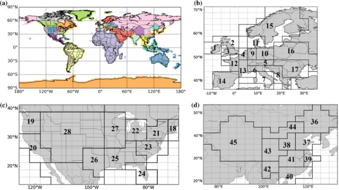
2.1.1. Control vector. We divide the globe, according to administrative boundaries, into a set of emitting regions whose monthly mean fossil fuel emission budgets are solved for during

a whole year (Fig. 1a). The corresponding space discretization

is higher in continents that have the largest emission densities

(Europe, US and China, Fig. 1b–d). The spatial resolution

in Europe is in agreement with the typical size of European countries. It is finer in western Europe where emissions can be high in specific regions such as northern Italy, southern England, eastern and western Germany. In the US and China, the spatial discretization is also increased in the most populated and industrialized areas (i.e. the east and west coasts in the US, and the south-eastern coast in China). In a given emitting

Fig. 1. (a) Map of the 56 regions whose monthly emission budgets are controlled by the inversion; (b) zoom on the 17 control regions in Europe; (c) zoom on the 11 control regions in the United States; (d) zoom on the 10 control regions in China.

country as done by Wang et al. (2013). In this study, the class ‘urban’ sites also include grid cells where large point sourc-es exist, e.g. power plants (based on the CARMAv2 database,

Ummel, 2012) and cement manufactures (Wang et al., 2013).

The name ‘urban’ is used for convenience. One more straight-forward approach would have been to select highest emitting grid cells according to EDG-IER with a threshold approximate-ly consistent with the one on the population as discussed above. But we prefer to keep a level of independency to this inventory and to its uncertainties by taking an independent proxy of the high emitting locations.

2.1.3. Observation operator. The observations are only influenced by the initial condition and the emissions during the year. As indicated above, the emissions are solved for by the inversion. Through diffusion by atmospheric transport, the

spatial gradients of FFCO₂ from a pulse of emissions at a given

time appear to become negligible (with an amplitude smaller than 0.1 ppm) within about 2 weeks, so that the influence of the global FFCO₂ distribution on 1 January 2007 (i.e. the initial condition of the inversion experiments in our studies) is quite

negligible for our simulations of gradients of FFCO₂ in Europe

in 2007, even for the results in January 2007 (not shown here). In our modelling of framework and corresponding simulations,

initial conditions for the FFCO₂ field in the atmosphere by the

1st day of the inversion year are thus ignored.

Consequently, the observation operator considered in this study is linear and does not bear an affine term y_fixed reflecting, in the observation gradients, the influence of a source or sink of

FFCO₂ that is not rescaled by our control vector. Therefore, it

can be denoted as H. We decompose it into:

In this formulation, H is a chain of three operators denot-ing the distribution of emissions within each region-month corresponding to the control variables (H_distr), the atmospheric

transport (H_transp), and the sampling of atmospheric gradients

(3)

𝐇= 𝐇samp𝐇transp𝐇distr

stations. Continuous measurement of total CO₂ has been

made for years in Europe (within the CarboEurope-IP, GHG-Europe and ICOS programs) and US (within the NOAA-ESRL framework) at tens of sites. A given radiocarbon measurement can be applied to a sample with any temporal integration time from 1 h to 1 month since air samples could be filled at

constant rates over long periods. However, the cost of the 14_CO

2

analysis of one sample is presently high so that monitoring of 14_CO

2 during a whole year favours the choice of integrated

samples at the daily to monthly scale (Levin, 1980; Turnbull

et al., 2009; Vogel et al., 2013). In this study, we only consider a single sampling frequency at all sites in each configuration of the observation vector. The two-week mean sampling is

considered as a standard sampling strategy in Section 4, while

the sensitivity to other sampling strategies will be discussed in

Section 5.2. We have also accounted for the technical ability

to have an intermittent filling (Levin et al., 2008; Turnbull

et al., 2016). Indeed, state-of-art inversion systems generally

make use of data during afternoon only due to limitations in modelling the vertical mixing during other periods of the day.

We thus assume that mean afternoon FFCO₂ observations are

sampled during 12:00–18:00 local time at the sites.

The locations of the stations where 14_CO

2 measurements are

made are assumed to be inland and distant from urban areas and other large sources, and aim to monitor the signature of the emissions at sub-continental scale. However, some sites will necessarily be closer to emitting areas (such as cities and power plants) than others, with consequences regarding the

rep-resentativeness and amplitude of the measured FFCO₂ signal.

We thus define two types of sites, both corresponding to land model grid cells: ‘urban’ and ‘rural’ sites, based on a threshold

on the population density (ORNL, 2015) within the grid cells

where the stations are located. This threshold is country-de-pendent and matches the World Bank urbanization data

(avail-able at http://data.worldbank.org/indicator/SP.URB.TOTL.

IN.ZS?page=1&order=wbapi_data_value_2011%20wba-pi_data_value%20wbapi_data_value-first&sort=asc) for each

of the atmosphere. We denote by 𝐇LMDZ

transp the resulting practical

implementation of H_transp.

(3) Observation sampling of the transport model outputs

In the observation operator, the practical simulation of FFCO₂

gradients corresponding to the observation vector relies on the simple extraction of individual concentration data at the meas-urement locations and then on the computation of differences between these concentration at different sites. We extract a concentration for a given location by taking the value in the transport model grid cell within which the site locates rath-er than intrath-erpolating values from sevrath-eral transport model grid cells. Usually, the height of the first level of LMDZ is about 150 magl. All the observations being assumed at 100 magl, they are all extracted from the first level of this version of LMDZ, except that of the reference site, Jungfraujoch (JFJ). JFJ is locat-ed at 3450 m above sea level (masl) but close to the ground level, at the top of a mountain. Since the LMDZ model poorly solves the topography in mountain areas, its ground level in the grid cell corresponding to JFJ is located far lower than this height. In order to ensure that the modelled concentrations are represent-ative of the free tropospheric air, JFJ observations are extracted from the sixth level of LMDZ, which is usually located between

2700 and 3800 masl. 1-day to 1-month mean afternoon FFCO₂

data are sampled in time by H_samp (depending on the

correspond-ing scorrespond-ingle observation frequency, see Section 2.1.2). We denote

by 𝐇coloc

samp the resulting practical implementation of Hsamp.

To sum up, the observation operator that will be used in practice for inversions in the following can be written

𝐇prac_{= 𝐇}coloc samp𝐇 LMDZ transp𝐇 PKU distr.

2.2. Theoretical derivation of the critical observation

errors

In this section, we are interested in decomposing the observa-tion error p(yo _{− Hx}t_|xt_{) for a typical H in order to isolate some}

critical sources of errors in practice. The observation operator

H = H_samp H_transp H_distr maps low-resolution budgets of the emis-sions into a coarse spatial grid. But each term of this operator is likely not perfectly represented in the following ways: (1) the products for the distribution of emissions within countries

such as the one used to build HPKU

distr are necessarily imperfect;

(2) the-state-of-the-art transport model such as the one used in 𝐇LMDZ

transp are necessarily imperfect; (3) the spatial

represent-ativeness of the measurements close to the ground can be low with coarse-resolution transport models and it can be difficult to represent the measurements in the vertical grid of the coarse-

resolution models (Broquet et al., 2011; Pillai et al., 2011)

which impacts the precision/accuracy of practical models for

H_samp H_transp. These add to the high measurement errors that have

to be accounted for when monitoring FFCO₂.

Focusing on these sources of errors, the term yo _{− Hx}t _{can be}

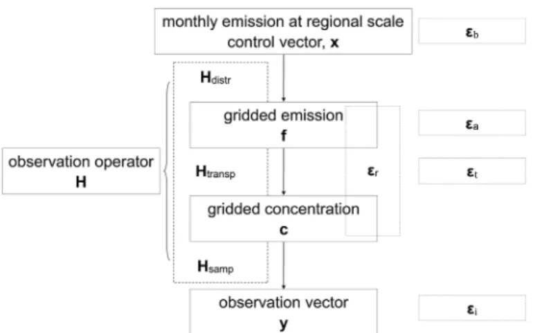
decomposed as follows: corresponding to the observation vector from the transport

model outputs (H_samp), respectively. The spatial and temporal

(sub-monthly) distribution operator x → f = Hdistr x distributes

the emission budgets for each region and month x into grid-ded emissions f at the spatial and temporal resolution expected as input of the atmospheric transport model. The atmospheric transport operator f → c = Htransp f simulates the FFCO2 field

c using an atmospheric transport model with prescribed

emis-sions f. The sampling operator c → y = Hsamp c applies the

atmospheric sampling procedure described above.

Each column of H represents the signature (the so-called response function) in the observation space of a unitary increment of the budget of the emissions in a given control

region-month. Fig. 2 gives the frame of the observation

opera-tor and its link to control and observation vecopera-tors.

For the observation operator used in practice, we use a coarse-grid transport model and emission inventories which catch the typical spatial and temporal large-scale variations in

the FFCO₂ emissions and concentrations and thus ensure the

realism of the typical estimates of uncertainties in our study. The corresponding products bear the typical precision/accuracy of the products that are used by state-of-the-art inversion

sys-tems when assimilating real data to quantify CO₂ natural fluxes

at large scale.

(1) Inventory used for the mapping of the emissions at high resolution

We use the PKU-CO₂-2007 global emission inventory for

2007 (Wang et al., 2013) to model, by the H_distr operator, the

spatial distribution of emissions within the regions of control.

PKU-CO₂-2007 is a high-resolution (0.1°) annual emission map

based on the disaggregation of national emission budgets using sub-national statistics. Regarding the sub-monthly temporal distribution of emissions within each month, we assume a flat temporal profile, as in many large-scale natural flux inversion systems (Peylin et al., 2013). We denote by HPKUdistr the practical implementation of the distribution operator H_distr.

(2) Global transport model configuration

An off-line version of the atmospheric general circulation model of Laboratoire de Météorologie Dynamique (LMDZ)

(version 4) (Hourdin et al., 2006) is used as our atmospheric

transport operator. The corresponding LMDZ simulation was nudged to the reanalysed wind fields from the European Cen-tre for Medium-Range Weather Forecasts (ECMWF) Interim

Reanalysis (ERA-Interim, (Berrisford et al., 2009)). LMDZ

has participated to a series of intercomparison exercises for

the simulation of CO₂ concentrations (Law et al., 2008) and

is able to reproduce most of the daily variations of the

large-scale transport of FFCO₂ (Peylin et al., 2011). The model

con-figuration used here has a horizontal resolution of 3.75° × 2.5° (longitude × latitude) and 19 hybrid sigma-pressure layers to discretize the vertical profile between the surface and the top

The total observation error ε_o defined by p(yo _{− Hx}t _{− y} fixed|xt)

can be expressed as:

Several of these terms are proportional to the value of xt _{while x}t

can take any value in the statistical framework of our inversion problem. This prevents, theoretically, from computing a fixed covariance R of the observation error assuming that this error can be represented by a distribution N(0, R). The configuration of such an error in the inversion systems generally ignore such a dependence of the model errors (transport, representation and aggregation errors) on the possible values for the actual fluxes which is a strong limitation for the application of the tradition-al data assimilation framework to flux inversion problems. In practice, we will derive R based on assumptions regarding the typical value for xt _{in our inversion cases.}

The errors on the different components of the observation operator relates to strongly different underlying input datasets

and different types of model (see Section 2.1.3) and are thus

considered to be independent. Assuming that they are all Gauss-ian and unbiased, one can write that ε_i ~ N(0, R_i), ε_r ~ N(0, R_r),

ε_t ~ N(0, R_t), ε_a ~N(0, R_a), and compute R as the sum of the covariances of the different errors:

Of note is that our formulations of the representation error and of the aggregation error are similar to the derivations of

representation error by Gerbig et al. (2003) and of aggregation

error by Engelen (2002), respectively. However, our formulation

of the aggregation error slightly differs from that of Kaminski et al. (2001) and Bocquet et al. (2011). We use a sort of ‘bot-tom-up’ approach to derive it, starting from the decomposition of the observation errors once having defined it as the sum of all sources of model data misfits other than the prior uncertainties and that are independent from these prior uncertainties. Kamin-ski et al. (2001) and Bocquet et al. (2011) rather followed what we consider as a ‘top-down’ approach to derive this aggregation error. Indeed, their introduction of the covariance of the aggre-gation error in the observation error covariance matrix ensures that the computation of the statistics for p(xt_|yo_{, x}b_{) is the same}

regardless of the control resolution. Due to the use of the usu-al assumption of the atmospheric inversion that the observation error is independent of the prior uncertainty, our ‘bottom-up’ (5)

𝝐

o= 𝝐i+ 𝝐r+ 𝝐t+ 𝝐a

(6) 𝐑= 𝐑i+ 𝐑r+ 𝐑t+ 𝐑a

where H_transpHR is a theoretical operator corresponding to the

linear transport from emissions f_HR to y, f_HR and this transport being represented using the ‘infinitely high’ resolution (i.e. continuously instead of using a discrete form) needed for catching all the patterns in the emissions and concentrations; Superscripts t denotes the true value of the emissions or observation operators at their corresponding space and time resolution (a ‘true observation operator’ meaning here a perfect operator without any model error). Even if this decomposition primarily aims at giving a physical characterization of each resulting term, it is also made such that these different terms can be assumed to be independent (see the justification for Equation (6) below).

We define the different terms of the observation error yo _{– Hx}t

based on this decomposition: (1) yo _{– H}t

transpHRf t

HR corresponds to the ‘measurement

error’ εi, which is associated with the precision of FFCO2

gradients derived from measurements of 14_{C and CO}

2.

The assumption given in section 1 that this precision is

1 ppm is discussed in Section 2.3. (2) Ht

transpHRf t

HR – Hsamp_Ht_transpHt_distrxt corresponds to the

rep-resentation error εr which arises from the modelling of

concentrations and emissions at the coarse resolution of the transport model in the observation operator. This error could be further split into errors due to missing high-resolution variations in the emissions at the model sub-grid scales, and errors due to comparing concentra-tions averaged at the model resolution to measurements

with a far lower spatial representativeness. Appendix A1

discusses such a decomposition, which, in practice, arti-ficially attributes most of the representation errors to the former or to the latter depending on the mathematical formulation. Therefore, even though this decomposition would have a physical meaning, it will be ignored here-after. (3) H_sampHt transpH t distrx t − H

sampHtransp_Ht_distrxt corresponds to the

transport errors εt due to the use of discretized and

sim-plified equation for modelling the transport. (4) H_sampH_transpHt

distrx

t – H

sampHtranspHdistrxt corresponds to the

aggregation error εa due to the imperfect representation

of the distribution of the monthly emissions within the region-months solved for by the inversion when using

H_distr. (4) 𝐲o−𝐇𝐱t =(𝐲o−𝐇t transpHR𝐟 t HR ) ⏟⏞⏞⏞⏞⏞⏞⏞⏞⏞⏞⏟⏞⏞⏞⏞⏞⏞⏞⏞⏞⏞⏟ 𝛆𝐢 +(𝐇t transpHR𝐟 t HR−𝐇samp𝐇 t transp𝐇 t distr𝐱 t) ⏟⏞⏞⏞⏞⏞⏞⏞⏞⏞⏞⏞⏞⏞⏞⏞⏞⏞⏞⏞⏞⏞⏞⏞⏞⏟⏞⏞⏞⏞⏞⏞⏞⏞⏞⏞⏞⏞⏞⏞⏞⏞⏞⏞⏞⏞⏞⏞⏞⏞⏟ 𝛆𝐫 +(𝐇_samp𝐇t transp𝐇 t distr𝐱 t −𝐇_samp𝐇_transp𝐇t distr𝐱 t) ⏟⏞⏞⏞⏞⏞⏞⏞⏞⏞⏞⏞⏞⏞⏞⏞⏞⏞⏞⏞⏞⏞⏞⏞⏞⏞⏞⏞⏞⏞⏞⏟⏞⏞⏞⏞⏞⏞⏞⏞⏞⏞⏞⏞⏞⏞⏞⏞⏞⏞⏞⏞⏞⏞⏞⏞⏞⏞⏞⏞⏞⏞⏟ 𝛆𝐭 +(𝐇_samp𝐇_transp𝐇t distr𝐱 t

−𝐇_samp𝐇_transp𝐇_distr𝐱t) ⏟⏞⏞⏞⏞⏞⏞⏞⏞⏞⏞⏞⏞⏞⏞⏞⏞⏞⏞⏞⏞⏞⏞⏞⏞⏞⏞⏞⏞⏞⏞⏟⏞⏞⏞⏞⏞⏞⏞⏞⏞⏞⏞⏞⏞⏞⏞⏞⏞⏞⏞⏞⏞⏞⏞⏞⏞⏞⏞⏞⏞⏞⏟

as a function of the model complicated and efforts have rather focused on the derivation of typical transport errors based on

the spread of different transport models (Law et al., 2008;

Peylin et al., 2011).

Finally, the errors in the measurements in our study should be fully independent of the inverse modelling framework.

The 1 ppm measurement error for FFCO₂ gradients between

sites corresponds to typical values based on the analysis of air samples by accelerator mass spectrometry (AMS) for

14_CO

2 (2–3‰, (Vogel et al., 2010; Turnbull et al., 2014)) and

by typical analyzers for continuous CO₂ samples (Chen et al.,

2010; Turnbull et al., 2011). Apart from these errors, various

fluxes that influence the atmospheric 14_CO

2, such as those from

cosmogenic production, ocean, biosphere and nuclear facilities,

make the direct conversion into FFCO₂ gradients bear complex

uncertainties whose typical values may exceed 1 ppm for some

locations and periods of times (Hsueh et al., 2007; Bozhinova

et al., 2013; Vogel et al., 2013). These additional sources of

uncertainties are not included in this study. In addition, we assume that all 14_CO

2 and CO2 samples will be analysed in the

same laboratory such as the present ICOS Central Radiocarbon Laboratory, or at least if the samples are measured by different instruments and laboratories, they will follow the official target of compatibility made by the World Meteorological

Organization (WMO) for 14_CO

2 measurements (GGMT-2013).

The consequence is that there should not be significant biases associated with instrumental errors impacting the gradients between sites analysed in this study.

3. Practical calculation of observation errors

In the inversion system, we use 𝐇prac= 𝐇colocsamp𝐇 LMDZ

transp𝐇

PKU distr as the observation operator. But here, we use a relatively independent representation of the ‘actual’ and higher resolution operators involved in the theoretical formulation of the observation errors

in Section 2.2 in order to derive an estimate of these errors.

These actual and higher resolution operators should bear pat-terns of the emissions, transport and concentration variability which should be realistic enough so that this estimate of the observation errors can provide a realistic characterization of the representation and aggregation errors when using real measure-ments.

A European configuration of the meso-scale transport model

CHIMERE (Schmidt et al., 2001) run with a 0.5° horizontal

res-olution, with 25 hybrid sigma-pressure vertical layers from the surface to the pressure altitude of 450 hPa, and with hourly con-centration outputs (to be aggregated into one-day to one-month mean afternoon data) is used to simulate HttranspHR and H

t transp. However, the LMDZ model is still used to model the practical

H_transp when calculating the aggregation error. The CHIMERE simulations are initialized at 50 ppm at 1 January 2007. method ignores potential correlations between the

aggrega-tion errors and the prior uncertainties, which is not the case of the ‘top-down’ approaches. Therefore, the formulations of the

covariance of the aggregation error in Kaminski et al. (2001)

and Bocquet et al. (2011) include a component related to this

correlation, which is ignored in our formulation. As discussed in

Appendix A2, we have nevertheless computed the corresponding

component and concluded that its weight is relatively small and negligible for our study. The mathematical details and a discus-sion regarding the potential correlations between the aggrega-tion errors and the prior uncertainties are given in Appendix A2.

2.3. Insights on the specificity or generality of the

observation errors investigated in this study

In theory, results for regions and months targeted by the inversion do not vary with the resolution of the control vector if the aggregation error εa is perfectly accounted for by R in the

inversion configuration (see the demonstration in the Appendix

based on the notations given above in Section 2.2). This

assumes that the uncertainty in the emissions at the scale of interest is independent of the uncertainty at higher resolution (which is approximately verified with our modelling set-up, see the Appendix). In other words, an inversion at coarse resolu-tion that accounts for aggregaresolu-tion errors εa should give the same

results for monthly fluxes over large regions as the same inver-sion applied to solve for hourly fluxes at the highest resolution (transport model grid). This is due to the equivalence between accounting for the uncertainties of fluxes within regions/month through their projection in the observation error or through their assigned prior uncertainty (given the assumptions underlying the inversion framework). In this sense, even though they are formally a function of the control vector, the aggregation errors at a scale larger than the transport model resolution are not spe-cific to a given inverse modelling set-up. Considering that the choice of the control resolution reflects a targeted resolution for the fluxes, aggregation errors rather reflect the impact for the monitoring of the fluxes at this targeted resolution of the uncer-tainties in the distribution of the fluxes at higher spatial or tem-poral resolutions. Increasing the control resolution would thus not, in theory, help solving for fluxes at the targeted resolution.

On the opposite, representation error is strongly linked to a specific inversion configuration. Increasing the resolution of the transport model used for the inversion necessarily de-creases them without a full compensation of this decrease by the rise of prior uncertainties. The transport errors should also depend on the transport modelling configuration. For example, synoptic patterns and the influence of the surface topogra-phy on the transport are better simulated at higher resolution. However, different transport models are also based on differ-ent parameterizations and computational approach, etc., which makes the quantification and evaluation of the transport errors

coarse representation of these emissions or of their signature outside Europe is negligible.

Htdistr (with outputs at 3° and 3-h resolution), the distribution

of ft

HR at 0.5° and 1-h resolution and x

t _{are modelled using the}

0.1° × 0.1° EDGARv4.2 2007 emission map (http://edgar.jrc.

ec.europa.eu) convoluted with temporal profiles (at 1-h resolu-tion) from IER (available at http://carbones.ier.uni-stuttgart.de/ wms/index.html). We denote this emission inventory EDG-IER afterwards. Aggregating this inventory at 1-h/0.5° resolution or at the scale of the inversion control region-month provides re-spectively fEDG-IER

HR and x

EDG-IER _{that are used to model f}t HR and x

t_.

Aggregating this inventory at 3-h/3° resolution (when comput-ing representation errors at the coarse transport resolution uscomput-ing CHIMERE) or 3-h/3.75° × 2.5° (when computing aggregation errors using LMDZ) and then rescaling it homogeneously with-in each region/month of control for the with-inversions to get unitary budget of emissions provides HEDG-IERdistr (using the same notation for the operator when the output ‘emission’ space is at 3° or 3.75° × 2.5° resolution) which is used to model Htdistr.

With these practical choices for modelling, the operators in-volved in the different types of observation errors defined in Section 2.2, the representation error writes:

and the aggregation error writes:

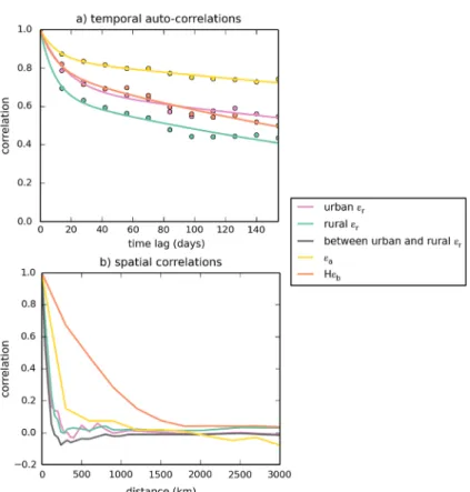
We only have one practical realization for each of these terms and thus of the corresponding errors, therefore, in order to derive their standard deviation and to investigate whether they bear potential temporal or spatial correlation, we make the strong assumption that the errors at different time and loca-tions have relatively similar statistical distribuloca-tions. However, this assumption of spatial and temporal homogeneity will be applied for adequate subset of observation time, locations and type, which will require a categorization of the observations.

Based on this assumption, we analyse the typical statistics of the representation and aggregation errors by using distributions of occurrences of these errors for different subsets (categories) of observations. Since observation sites of continental networks could locate in any grid cell, all the spatial grid cells and all one-day to one-month afternoon time windows are used and categorized among different subsets for this analysis. The dif-ferent spatial and temporal categories will be defined based on the analysis of the spatial and temporal variations of the errors. The potential temporal auto-correlations and spatial correla-tions within/across categories are also analysed.

Using a similar approach, transport errors could have

been evaluated using 𝐇coloc

samp𝐇 CHIM transp𝐇 EDG-IER distr 𝐱 EDG-IER _and 𝐇coloc samp𝐇 LMDZ transp𝐇 EDG-IER distr 𝐱

EDG-IER _{. However, the spatial resolution}

and orography of HCHIM

transp and 𝐇

LMDZ

transp are not exactly the same

and this could have artificially increased the transport error with representation error. Therefore, we make a simpler estimation (7) 𝐇CHIM_transpHR𝐟_HREDG-IER−𝐇colocsamp𝐇

CHIM transp𝐇 EDG-IER distr 𝐱 EDG-IER (8) 𝐇coloc_samp𝐇LMDZ_transp𝐇EDG-IER_distr 𝐱EDG-IER−𝐇colocsamp𝐇

LMDZ

transp𝐇

PKU distr𝐱

EDG-IER

We model HttranspHR by feeding CHIMERE with 0.5°

resolu-tion maps of the emissions and using the one-day to one-month mean afternoon 0.5°-resolution and 25 vertical-level

concen-tration fields to extract simulated gradients of FFCO₂. Since

the resolution of this CHIMERE configuration is not infinitely high, in practice, a sampling operator is still needed to

mod-el HttranspHR . The vertical resolution of CHIMERE being about

35–45 m for the first three levels, the 100 magl observations

involved in the computation of the FFCO₂ gradients at high

resolution are extracted in the third level of this model (and in the 0.5° horizontal model grid cell containing the horizontal position of the stations, using a sampling option similar to that used in 𝐇coloc_samp). The FFCO₂ concentrations at the reference site are extracted from the 23rd vertical level of CHIMERE cor-responding to the altitude of 3450 masl in the 0.5° grid cell where the reference site located. This transport (and sampling) configuration that is used to model HttranspHR is denoted H

CHIM transpHR. By degrading the horizontal and temporal resolution of the emissions in input of the CHIMERE model and by averaging (horizontally and vertically) the mole fractions in output of the

CHIMERE simulations we model Httransp. The spatial

aggrega-tion of the CHIMERE outputs consists first in a vertical ag-gregation, and then on a horizontal aggregation. The horizontal aggregation does not fully correspond to an aggregation within the LMDZ grid cells (i.e. to the interpolation of the 0.5° res-olution fields for CHIMERE into the 3.75° × 2.5° resres-olution grid of LMDZ). For simplicity, the 0.5° CHIMERE grid cells are rather aggregated from blocks of 6 × 6 grid cells to yield coarse grid at the 3° resolution which is close to that of the LMDZ grid. HCHIMtransp denotes the configuration where CHIMERE is fed with emissions maps aggregated at 3° resolution (close to that of the LMDZ model) and over 3-h time windows, and where CHIMERE one-day to one-month mean afternoon out-put concentrations are, again, aggregated at 3° resolution. For

the modelling of H_samp in the computation of the error due to

aggregation at the transport model resolution and in the com-putation of the representation error we apply an operator which follows the principle of 𝐇coloc_samp (and which we will thus also de-note 𝐇coloc_samp) i.e. FFCO₂ observations are extracted in the first aggregated vertical levels for all the sites but the reference site, which is extracted in the sixth aggregated vertical level, and in the co-located aggregated 3° horizontal grid cells of the HCHIMtransp outputs. When calculating the error due to the aggregation at region-month scale, we use 𝐇coloc_samp to model H_samp and apply it to 𝐇LMDZ_transp.

Associating CHIMERE at 0.5° resolution with HttranspHR (and

consequently 0.5° resolution maps of the emissions with ftHR)

assumes that the main variations (i.e. those which have the larg-est impact for data at 100 magl) of emissions or concentrations within 3° resolution grid cells occur at scales larger than 0.5°. Furthermore, simulating HttranspHR and H

t

transp with CHIMERE

which is a regional model (over Europe) assumes that the aggregation and representation errors in Europe due to the

of the transport error statistics for the daily afternoon mean

FFCO₂. Transport errors for daily to monthly mean afternoon

FFCO₂ are then derived based on the value obtained for daily

afternoon mean FFCO₂ and on the above mentioned

assump-tion that there is no temporal auto-correlaassump-tion of the transport errors between afternoon mean concentrations in different days. For example, our estimate of the transport error for two-week mean afternoon concentrations (mean of 14 days) is equal to1.74× 1.34∕√14= 0.62 ppm at SAC site.

Following this estimation, the transport error in the two-week

mean afternoon FFCO₂ concentration at JFJ site is 0.21 ppm.

The transport error in the one-day to one-month mean afternoon

FFCO₂ gradients between any site and JFJ is calculated

assum-ing no spatial correlation of the transport errors between sites, i.e. as √(ε2

t,i+ε 2

t,JFJ) where εt,i is the transport error for

concentra-tions at site i and εt,JFJ is the transport error in concentrations

at site JFJ at the corresponding one-day to one-month scale. As a result, the transport errors in the two-week mean

after-noon FFCO₂ gradients from 100 magl sites to the JFJ reference

site range from 0.42 to 1.07 ppm. The transport errors in the

one-day mean afternoon FFCO₂ gradients range from 1.58 to

3.99 ppm (and from 0.29 to 0.74 ppm in the case of errors on

1-month mean afternoon FFCO₂ gradients, respectively).

As indicated in Section 2, we also want to compare the

observation errors to the projection of the prior uncertainty in the observation space p(H(xt _{− x}b_)|xb_{) denoted Hε}

b (and called

‘prior FFCO₂ errors’ hereafter, εb corresponding to the prior

uncertainties). Following the same approach as for the estima-tion of the representaestima-tion and aggregaestima-tion errors, and setting xb_,

as in the companion inversion studies, with emission budgets

from PKU-CO₂-2007 (hereafter xPKU_{), we derive estimates of}

Hεb based on statistics on Hprac(xEDG-IER − xPKU).

4. Results: estimates of the representation and

aggregation errors

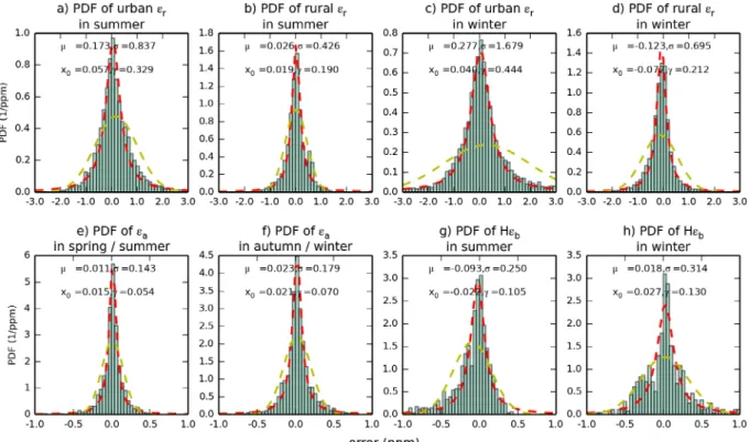
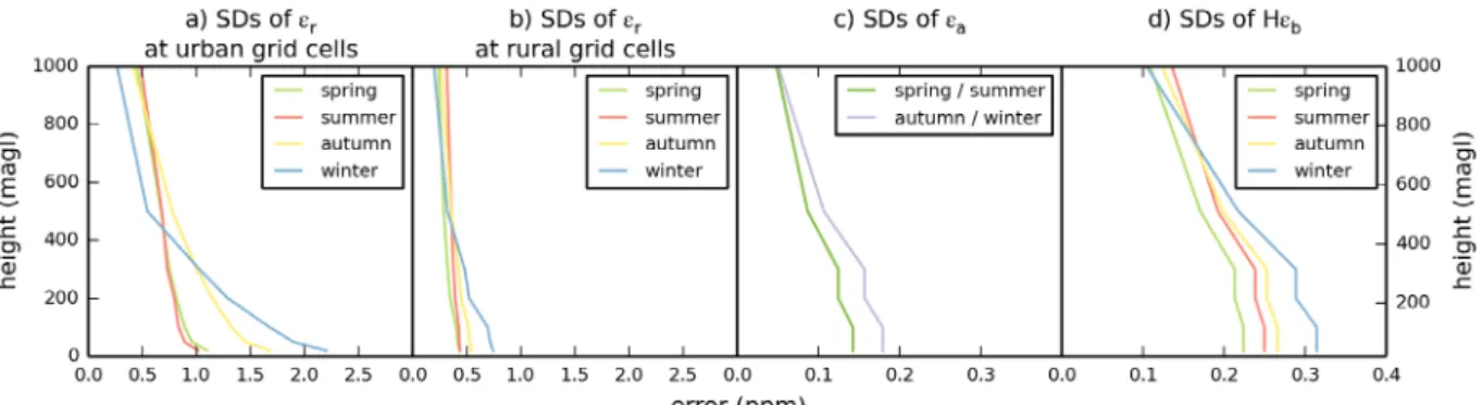
This Section characterizes the representation, aggregation and

prior FFCO₂ errors, derived from the method described in

Sec-tion 3. This characterization consists in providing their typical values (estimates of their standard deviations), investigating whether they bear temporal or spatial correlations while such correlations of the observation errors are traditionally ignored

by atmospheric inversions (Rödenbeck et al., 2003; Chevallier

et al., 2005; Peylin et al., 2013), and in investigating the validity of the assumptions that these observation errors have

Gaussi-an Gaussi-and unbiased distributions. Section 4 focuses on the errors

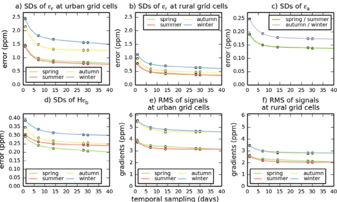
for a standard sampling strategy i.e. two-week mean afternoon

sampling at 100 magl. Section 5 will explore the sensitivity of

the results to the temporal sampling strategy (from one-day to one-month mean afternoon sampling) and give insights on the errors that would have been obtained if considering measure-ments sites with a different measurement height.

of the transport errors for simulated FFCO₂ gradients based on

that of transport errors for simulated FFCO₂ at individual sites. For this estimation, we make several assumptions. First, we assume that there is no temporal auto-correlation of the transport error in simulated daily mean afternoon concentrations between different days at a given location. This assumption, however, may be violated if there are significant biases in the simulation of the meteorological conditions, i.e. the planetary boundary layer height and the vertical mixing strength (Miller et al.,

2015; Basu et al., 2016). Nevertheless, the estimate of the

structure of the temporal auto-correlations of the transport error

is challenging (Lin and Gerbig, 2005; Lauvaux et al., 2009;

Miller et al., 2015) and there is no clear evidence that such

autocorrelations is significant at daily scale (Lin and Gerbig,

2005; Lauvaux et al., 2009; Broquet et al., 2011). In this study, we follow the assumption made by the majority of existing inversion studies (Peters et al., 2007; Chevallier et al., 2010; Niwa et al., 2012; Peylin et al., 2013), in which the temporal auto-correlations in the transport error are usually ignored. Second, we assume that the standard deviation of the transport error in simulated daily mean afternoon concentrations is constant in time at a given location. Finally, we assume that the ratio between this standard deviation and the temporal standard deviations of the 1-year long time series of the high-frequency variability of the detrended and deseasonalized simulated daily mean afternoon concentrations in the corresponding grid cell of the transport model is constant in space (i.e. that this ratio is identical for all grid cells of the transport model). The high-frequency variability is calculated by the method of Thoning

et al. (1989). The underlying assumption is that the transport

models should be less reliable at sites where the concentrations have a larger variability (Peylin et al., 2005; Geels et al., 2007).

These assumptions allow us to use the station of Saclay (SAC) near Paris for deriving a generalized estimate of the ratio

between the transport errors and the simulated FFCO₂ temporal

variability. According to Peylin et al. (2011), the annual

aver-age of the standard deviations between simulated hourly mean FFCO₂ concentrations at this site from a set of state-of-the-art transport models is 2.34 ppm. We use this value to define the standard deviation of the transport errors associated with the simulated daily afternoon mean concentrations. The standard deviation of the one-year long-time series of the daily afternoon mean concentrations simulated within one year with our practi-cal implementation of the simulation of 3-hourly concentrations 𝐇LMDZ

transpH EDG-IER

distr x

EDG-IER _{at SAC is 1.74 ppm. So the ratio between}

the standard deviation of the transport error for daily afternoon mean concentrations and the standard deviation of simulated time series for the daily afternoon mean concentrations within one year for any site is assumed to be 2.34/1.74 = 1.34. For any potential sites (in any grid cells in LMDZ), we thus multiply this ratio by the standard deviation of the simulated daily after-noon mean concentrations within one year to get an estimate

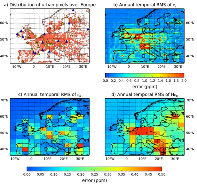
Fig. 3b–d. In general, the RMS of the representation error for land grid cells ranges between 0.4 and 4.0 ppm across Europe,

while the RMS of the aggregation and prior FFCO₂ errors are

much smaller.

From Fig. 3b, the representation error at 100 magl shows

higher values in the grid-cells classified as urbanized and large cities such as London, Paris, industrialized areas in Germany, etc. More generally, the spatial distribution of representation error shows a good consistency with the mask of the urban grid cells defined based on the population density and large point sources (Fig. 3a, see its definition in Section 2.1.2), indicating higher representation error in urban grid cells. We conclude that different statistics of the representation error need to be derived for the ‘urban’ 0.5° resolution land grid cells of the mask in

Finally (in Section 6), we compare the typical values of the

representation, aggregation and prior FFCO₂ errors to the

mod-el transport errors (derived in Section 3), to the measurements

errors (given in the introduction), and to the typical signal of

FFCO₂ modelled at the sites considered in this study.

4.1. Spatial distribution of the errors and spatial

categorization

The root mean square (RMS) of the representation,

aggrega-tion and prior FFCO₂ errors for the one-year long time-series

of two-week mean FFCO₂ gradients at each of the 0.5° to

3.5° × 2.75° horizontal grid cells (depending on the error and thus on the scale at which it can be computed) are given in

Fig. 3. Distribution of urban pixels (defined by population density, section 2.1.2) over Europe at 0.5° resolution (a) and maps of the RMS of the 1-year long time series of the representation errors εr (at 0.5° resolution) (b) εa (at 3.75°× 2.5° resolution) (c) and the prior FFCO2 errors Hεb

(at 3.75°× 2.5° resolution) (d) for 2-week mean afternoon FFCO₂ gradients (from 100 magl sites to the JFJ reference site) (unit: ppm). In (a), the triangles give the location of the sites of a typical continental observation network similar to ICOS (ICOS, 2008; 2013); blue triangles means that the stations are in ‘rural’ pixels, while yellow triangles means the stations fall in ‘urban’ pixels.