HAL Id: hal-01155075
https://hal.archives-ouvertes.fr/hal-01155075v2
Submitted on 2 Jun 2015
HAL is a multi-disciplinary open access
archive for the deposit and dissemination of
sci-entific research documents, whether they are
pub-lished or not. The documents may come from
teaching and research institutions in France or
abroad, or from public or private research centers.
L’archive ouverte pluridisciplinaire HAL, est
destinée au dépôt et à la diffusion de documents
scientifiques de niveau recherche, publiés ou non,
émanant des établissements d’enseignement et de
recherche français ou étrangers, des laboratoires
publics ou privés.
Bayesian Personalization of Brain Tumor Growth Model
Matthieu Lê, Hervé Delingette, Jayashree Kalpathy-Cramer, Elizabeth
Gerstner, Tracy Batchelor, Jan Unkelbach, Nicholas Ayache
To cite this version:
Matthieu Lê, Hervé Delingette, Jayashree Kalpathy-Cramer, Elizabeth Gerstner, Tracy Batchelor, et
al.. Bayesian Personalization of Brain Tumor Growth Model. MICCAI - Medical Image Computing
and Computer Assisted Intervention - 2015, Oct 2015, Munich, Germany. pp.424-432,
�10.1007/978-3-319-24571-3_51�. �hal-01155075v2�
Bayesian Personalization of
Brain Tumor Growth Model
Matthieu Lˆe1, Herv´e Delingette1, Jayashree Kalpathy-Cramer2, Elizabeth R. Gerstner3, Tracy Batchelor3, Jan Unkelbach4, and Nicholas Ayache1
1
Asclepios Project, INRIA Sophia Antipolis, France
2 Martinos Center for Biomedical Imaging, Harvard–MIT Division of Health Sciences
and Technology, Charlestown, MA, USA
3 Department of Neurology, Massachusetts General Hospital, Boston, Massachusetts,
USA
4 Department of Radiation Oncology, Massachusetts General Hospital and Harvard
Medical School, Boston, MA, USA
Abstract. Recent work on brain tumor growth modeling for glioblas-toma using reaction-diffusion equations suggests that the diffusion coeffi-cient and the proliferation rate can be related to clinically relevant infor-mation. However, estimating these parameters is difficult due to the lack of identifiability of the parameters, the uncertainty in the tumor segmen-tations, and the model approximation, which cannot perfectly capture the dynamics of the tumor. Therefore, we propose a method for conduct-ing the Bayesian personalization of the tumor growth model parameters. Our approach estimates the posterior probability of the parameters, and allows the analysis of the parameters correlations and uncertainty. More-over, this method provides a way to compute the evidence of a model, which is a mathematically sound way of assessing the validity of dif-ferent model hypotheses. Our approach is based on a highly parallelized implementation of the reaction-diffusion equation, and the Gaussian Pro-cess Hamiltonian Monte Carlo (GPHMC), a high acceptance rate Monte Carlo technique. We demonstrate our method on synthetic data, and four glioblastoma patients. This promising approach shows that the infiltra-tion is better captured by the model compared to the speed of growth.
1
Introduction
Glioblastomas (GBM) are one of the most common types of primary brain tu-mors. In addition to being infiltrative by nature, they are also the most aggressive of brain tumors. Reaction-diffusion equations have been widely used to model the GBM growth, using a diffusion and a logistic proliferation term,
∂u ∂t = ∇(D.∇u)| {z } Diffusion + ρu(1 − u) | {z } Logistic Proliferation (1) D∇u.−→n∂Ω= 0 (2)
Fig. 1: For the two time points: a) T1Gd with the abnormality segmented in orange. b) T2-FLAIR with the abnormality segmented in red. c) Tumor cell density using the maximum a posteriori parameters with the 80% and 16% threshold outlined in black. d) Comparison between the clinician segmentations and the model segmentations.
Equation (1) describes the spatio-temporal evolution of the tumor cell density u, which infiltrates neighboring tissues with a diffusion coefficient D, and prolif-erates with a net proliferation rate ρ. Equation (2) enforces Neumann boundary conditions on the brain domain Ω. Equation (1) admits solutions which asymp-totically behave like traveling waves with speed v = 2√Dρ and infiltration length λ =pD/ρ [1]. The infiltration length is related to the spatial rate of decay of the density u. Preliminary works suggest that D and ρ can help in assessing the response to therapy [2].
The personalization of D and ρ is based on serial acquisitions of Magnetic Resonance Images (MRIs). The tumor causes abnormalities on T1 post Gadolin-ium (T1Gd) and T2-FLAIR MRIs, which can be monitored over time. To relate the tumor cell density u to those images, it is usually assumed that the visible borders of these abnormalities correspond to a threshold of the tumor cell den-sity [1]. Since the T2-FLAIR abnormality is larger than the T1Gd abnormality, the T2-FLAIR abnormality borders correspond to a lower threshold of tumor cell density (Fig. 1). Therefore, given MRIs of a patient at 2 time points, it is possible to extract the segmentations of the 4 visible abnormalities. Those can be used to personalize a tumor growth model, i.e. to find the set of parameters θ = (D, ρ) which best fits those segmentations.
This problem was studied by Harpold et al. [1] who described a heuristic to re-late the volumes of the four available segmentations to the speed v = 2√Dρ and infiltration length λ =pD/ρ, based on the asymptotic behavior of the solutions of equation (1), hence allowing for the personalization of D and ρ. Konukoglu et al. [3] also elaborated a personalization strategy based on BOBYQA, a state-of-the-art derivative-free optimization algorithm. However, this latter method only considers one MRI modality per time point, and fails to simultaneously identify D and ρ. These estimation procedures provide single-solutions which are sensi-tive to the initialization, and do not provide any understanding about potential correlation between parameters.
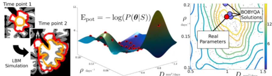
Fig. 2: a) Two synthetic time points with the simulated T1Gd and T2-FLAIR abnormalities (orange and red resp.). b) Gaussian process interpolation of Epot
using the evaluation of the posterior at well chosen points (in red). c) Kernel density estimate of the posterior using 1000 samples. Results of the BOBYQA optimization with multiple initializations in blue, true parameters in red.
To circumvent these drawbacks, we propose a method to estimate the poste-rior probability of θ = (D, ρ) from the T1Gd and T2-FLAIR abnormalities at 2 time points. We show how this method provides information on the confidence in the estimation, and provides a global understanding of the correlation between the parameters. We further demonstrate how the knowledge of the posterior distribution can be used to compare different model hypotheses. The method is based on the computation of the statistical evidence: the probability of ob-serving the data given the model. The Bayes factor, defined as the ratio of the evidence of two different models, allows one to compare the models and select which better explains the data. This idea is applied to determine which tumor cell density threshold is the most adequate for the T2-FLAIR abnormality.
Naive Monte Carlo would be impractical due to computational overload. Some strategies rely on approximations of the posterior probability with sparse grids [4], approximations of the forward model based on reduced order models [5,6], or on expensive grid methods [7]. We present here a method based on the highly parallelized implementation of the reaction-diffusion equation using the Lattice Boltzmann Method (LBM), and the Gaussian Process Hamiltonian Monte Carlo (GPHMC), a high acceptance rate Monte Carlo technique.
2
Method
2.1 Tumor Growth Model
We consider the model defined in equations (1,2). Following previous work [1], the diffusion tensor is defined as D = dwI in the white matter and D = dw/10 I
in the gray matter, where I is the 3x3 identity matrix. We further identify the pa-rameter D with dw. As such, the diffusion is heterogeneous and locally isotropic.
This model reproduces the infiltrative nature of the GBM, takes into account anatomical barriers (ventricles, sulci, falx cerebri), and the tumor’s preferential progression along white matter tracts such as the corpus callosum. The reaction-diffusion equation is implemented using the Lattice Boltzmann Method (LBM)
[8]. The LBM are parallelized such that simulating 30 days of growth, with a time step of 0.1 day, takes approximately 80 seconds on a 60 core machine for a 1mm isotropic brain MRI. The initialization of the tumor cell density u(t = t1, x) at
the time of the first acquisition is of particular importance, as it impacts the rest of the simulation. In this work, the tumor tail extrapolation algorithm described in [9] is used. The tumor cell density is computed outward (and inward) of the T1Gd abnormality borders as a static approximation of the wave-like solution of equation (1) with parameter θ. Consequently, the T1Gd abnormality falls exactly on the threshold of the tumor cell density at the first time point.
2.2 GPHMC
Given parameter θ, the model is initialized by extrapolating the tumor cell density from the T1Gd segmentation at time t1. Its dynamics is then
simu-lated using the LBM until time t2. The thresholded tumor cell density is then
compared to the segmentations S of the T1Gd at time t2 and the T2-FLAIR
at time t1 and t2 (Fig. 1). To cast the problem in a probabilistic framework,
we follow Bayes rule: P (θ|S) ∝ P (S|θ) P (θ). The likelihood is modeled as P (S|θ) ∝ exp(−d(S, u)2/σ2), where the distance d(S, u) is the mean
symmet-ric Hausdorff distance between the border of the segmentations S and the isolines of the simulated tumor cell density u. The noise level is quantified through σ. Samples are drawn from the posterior probability using the Gaussian Process Hamiltonian Monte Carlo [10].
Hamiltonian Monte Carlo (HMC). HMC is a Markov Chain Monte Carlo algorithm which uses a refined proposal density function based on the Hamiltonian dynamics [10]. The problem is augmented with a momentum vari-able p ∼ N (0, I). By randomly sampling p, we define the current state (θ, p). HMC is designed to propose a new state (θ∗, p∗) with constant energy H = Epot+ Ekin, with potential energy Epot = − log(P (S|θ)P (θ)), and kinetic
en-ergy Ekin= 1/2 ||p||22. The new state is the result of the Hamiltonian dynamics:
dθi/dt = ∂H/∂pi and dpi/dt = −∂H/∂θi. The new state (θ∗, p∗) is accepted
with probability A = min [1, exp(−H(θ∗, p∗) + H(θ, p)]. The conservation of the
energy during the Hamiltonian dynamics, up to the numerical discretization ap-proximation, insures a high acceptance rate A.
Gaussian Process Hamiltonian Monte Carlo (GPHMC). In the HMC, computing the Hamiltonian dynamics requires a significant amount of model eva-lutations. To circumvent this difficulty, Epot is approximated with a Gaussian
process [10] (Fig. 2). During an initialization phase, Epotis evaluated by running
the forward model at random locations. Those evaluation points are used to de-fine the Gaussian process approximating Epot- details in [10]. HMC is then run
using the Gaussian process interpolation of Epot to compute the Hamiltonian
dynamics. Given that the Gaussian process well captures Epot, the GPHMC
benefits from the high acceptance rate of the HMC.
Posterior Density. P (θ|S, M) is computed using a kernel density estima-tion on the drawn samples {θi}Ni=1. A bounce-back boundary condition is applied
2.3 Bayes Factor: Extension of the Chib’s Method
The evidence of the model M can be expressed using Chib’s method [11]
P (S|M) = P (S|θ, M)P (θ|M) P (θ|S, M) ∝ exp(− d(S, Yθ)2 σ2 ) P (θ|M) P (θ|S, M) (3) In other words, the probability of observing the segmentation given the model (evidence) is equal to the likelihood times the prior, normalized by the posterior. The Chib’s method evaluates this equation on a sample θ of high posterior probability, like its mode. We propose instead a more robust estimation of the evidence, as an extension of the Chib’s method, by averaging it over the samples {θi}Ni=1 drawn from the posterior distribution,
P (S|M) = Eθ|S,M[P (S|M)] ∝ 1 N N X i=1 exp(−d(S, Yθi) 2 σ2 ) P (θi|M) P (θi|S, M) (4)
This estimator is less prone to errors when the kernel density estimation of the posterior approximately captures the real density at the modes. In order to compare two models M1 and M2, we can compute the Bayes factor B =
(P (S|M1)P (M1))/(P (S|M2)P (M2)). If B is substantially larger than 1, it is
evidence that M1is better suited to explain the data than M2. This is a Bayesian
alternative to the frequentist hypotheses testing approach.
3
Experiments and Results
We present results on synthetic and real data. The tumor cell density visibility thresholds are assumed to be 80% for the T1Gd abnormality and 16% for the T2-FLAIR abnormality [12]. The parameters are constrained such that D ∈ [0.02, 1.5] mm2/days, and ρ ∈ [0.002, 0.2] days−1[1]. The prior P (θ) is assumed uniform within this bounded box. After trials, the noise level has been manually tuned to σ = 10 mm. Our results are compared to the direct minimization of d(S, Y ) using BOBYQA. BOBYQA is run 9 times with 9 different initializations in the parameter space - around 20 iterations per BOBYQA were observed. Finally, we compare two models using two different tumor cell density visibility thresholds for the T2-FLAIR abnormality frontier: 16% for the first model M1,
and 2% for the second model M2, following different studies [1]. The Bayes
factor between M1and M2 is computed to compare the models.
Synthetic Data. Starting from a manually drawn T1Gd abnormality seg-mentation, the growth of a tumor is simulated on an atlas of white and gray mat-ter during 30 days with D = 1.0 mm2.days−1and ρ = 0.18 days−1. The first and
last images are thresholded in order to define the 4 segmentations (Fig. 2 left). 1000 samples are drawn with the GPHMC, using a GP interpolation of Epotwith
35 points (Fig. 2 middle). The acceptance rate is 90%, demonstrating that the Gaussian process successfully captured Epot. The best BOBYQA solutions are
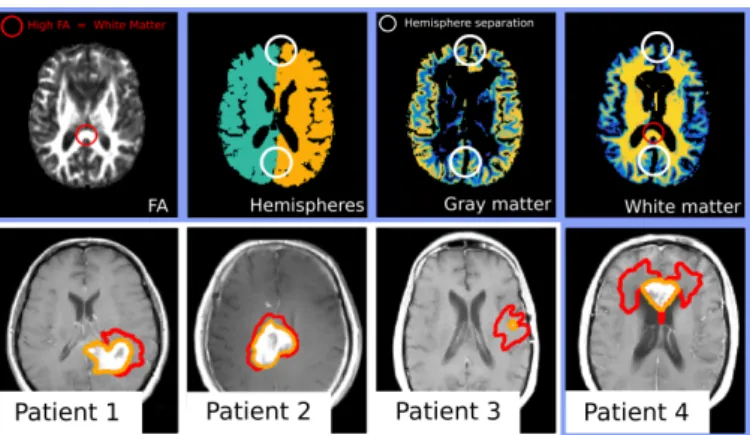
Fig. 3: Top: Data processing using the Fractional Anisotropy (FA) and the hemi-sphere segmentation to ensure the separation of the hemihemi-spheres in the white and gray matter. Bottom: T1Gd of the 4 real cases for the first time point. The T1Gd (resp. T2-FLAIR) abnormality is outlined in orange (resp. red).
BOBYQA solutions somewhat distant from the true solution, demonstrates the need for multiple initializations of the algorithm. The true parameter is outlined by high posterior density isocontour, and the posterior reflects little correlation between the parameters (unimodal and somewhat peaked posterior). Finally, with equation (4), we computed a Bayes factor B = P (S|M1)/P (S|M2) = 3,
indicating that M1 is better suited than M2 in the synthetic case.
GBM Cases. The method is applied to the 4 GBM patients shown in Fig. 3 (bottom panel). The T1Gd and T2-FLAIR abnormalities are segmented by a clinician. For each time point, the T2-FLAIR is rigidly registered to the T1Gd. The rigidly registered T2-FLAIR at time t2 is then non-linearly registered to
the T2-FLAIR at time t1. All the segmentations are then mapped to the T1Gd
image space at time t1 where the white matter, gray matter and cerebrospinal
fluid (CSF) are segmented (Fig. 3 top panel). Close attention is paid to the sepa-ration of the hemispheres to prevent tumor cells from invading the contralateral hemisphere. Voxels at the boundary of the hemispheres that show low Fractional Anisotropy value are tagged as CSF to ensure the separation of the hemispheres, while keeping the corpus calosum as white matter (Fig. 3).
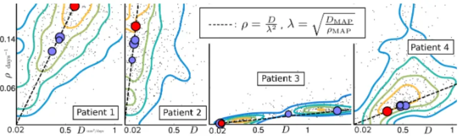
The mean acceptance rate for the 4 patients is 74% (Fig. 1) which shows that the Gaussian process successfully interpolate Epot. The BOBYQA solutions,
al-though reasonable, fail to describe the spatial dynamics of the posterior (Fig. 4). This emphasizes the need for a global understanding of the posterior’s behavior. We see that the model can capture the infiltration length of the tumor growth: the posterior is elongated along the line of constant infiltration λ =pD/ρ, es-pecially for patients 1, 2 and 3 (see the black dashed line on Fig. 4). A small infiltration λ corresponds to a T2-FLAIR abnormality close to the T1Gd abnor-mality (patient 1 Fig. 3) while a larger infiltration corresponds to more distant abnormalities (patient 4 Fig. 3). However, the model less successfully captures
Fig. 4: Posterior estimation for the 4 real cases. The blue dots are the three best BOBYQA solutions. The red dot is the maximum a posteriori of the drawn samples θMAP. The dashed black line is the line of constant infiltration ρ = D/λ2.
the speed of the growth, as the posterior does not present a clear mode on the constant infiltration line. For patient 3, the presence of two modes suggests that the speed of growth might be explained by two sets of parameters. Moreover, the presence of two modes is responsible for the relatively low acceptance rate of 51%. The posterior distribution is more complex and therefore harder to in-terpolate with the Gaussian process. For patient 4, the posterior is more peaked and suggests that both the infiltration and speed can be explained by the model. The simulation corresponding to the sample θ of lowest potential energy Epotis
presented on Fig. 1 (right). We note θMAP= (DMAP, ρMAP) the drawn sample
corresponding to the lowest potential energy Epot. It is interesting to note that
θMAPcan be slightly skewed on the edge of high posterior isocontour (patient 3
or 4 on Fig. 1). This is caused by the very high sensitivity of the output to the parameters’ value, as well as the likelihood model which allows for a certain noise level σ. The Bayes factor between M1 and M2 was computed for the different
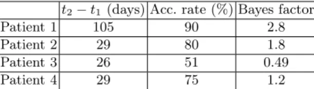
patients (Fig. 1). We can see that for patients 1, 2, and 4, the Bayes factor leans toward validating the model M1 with a mean of 1.9. Patient 3 presents a lower
Bayes factor supporting model M2, but this patient presents an odd posterior,
which might indicate that the reaction-diffusion model less successfully captures the dynamics of the growth.
4
Conclusion
We presented a Bayesian personalization of the parameters of a tumor growth model on 4 patients. The computation of the posterior provides far more in-formation than the direct optimization, and takes only five times longer. Our method provides a global understanding of the correlation between the param-eters, and we showed that the model captures the infiltration way better than the speed of growth of the tumor. Furthermore, it provides a way to compute the Bayes factor and compare the validity of different model hypotheses, which showed that a threshold of 16% was probably better suited for the data. In the future, we want to apply this methodology to larger dimensional problems. Namely, the noise level σ could be included as an unknown, and depend on the
t2− t1 (days) Acc. rate (%) Bayes factor
Patient 1 105 90 2.8
Patient 2 29 80 1.8
Patient 3 26 51 0.49
Patient 4 29 75 1.2
Table 1: Presentation of the patients.
image modality. Finally, we believe that such a method could be applied to per-sonalized treatment planning.
Acknowledgments. Part of this work was funded by the European Research Council through the ERC Advanced Grant MedYMA 2011-291080.
References
1. Harpold, H.L., Alvord Jr, E.C., Swanson, K.R.: The evolution of mathematical modeling of glioma proliferation and invasion. J. of Neurop. & Exp. Neurol. (2007) 2. Neal, M.L., Trister, A.D., Ahn, S., Baldock, A., et al.: Response classification based on a minimal model of GBM growth is prognostic for clinical outcomes and distinguishes progression from pseudoprogression. Cancer research (2013) 3. Konukoglu, E., Clatz, O., Menze, B.H., Stieltjes, B., Weber, M.A., Mandonnet,
E., et al.: Image guided personalization of reaction-diffusion type tumor growth models using modified anisotropic eikonal equations. MedIA 29(1) (2010) 77–95 4. Menze, B.H., Van Leemput, K., et al.: A generative approach for image-based
modeling of tumor growth. In: IPMI, Springer (2011) 735–747
5. Konukoglu, E., Relan, J., Cilingir, U., Menze, B.H., Chinchapatnam, P., Jadidi, A., et al.: Efficient probabilistic model personalization integrating uncertainty on data and parameters: Application to eikonal-diffusion models in cardiac electro-physiology. Progress in biophysics and molecular biology 107(1) (2011) 134–146 6. Neumann, D., Mansi, T., Georgescu, B., Kamen, A., Kayvanpour, E., Amr, A.,
et al.: Robust image-based estimation of cardiac tissue parameters and their un-certainty from noisy data. In: MICCAI 2014. Springer (2014) 9–16
7. Wallman, M., Smith, N.P., Rodriguez, B.: Computational methods to reduce un-certainty in the estimation of cardiac conduction properties from electroanatomical recordings. MedIA 18(1) (2014) 228–240
8. Yoshida, H., Nagaoka, M.: Multiple-Relaxation-Time LBM for the convection and anisotropic diffusion equation. Journal of Computational Physics 229(20) (2010) 9. Konukoglu, E., Clatz, O., Bondiau, P.Y., Delingette, H., Ayache, N.:
Extrapolat-ing glioma invasion margin in brain magnetic resonance images: SuggestExtrapolat-ing new irradiation margins. MedIA 14(2) (2010) 111–125
10. Rasmussen, C.E.: Gaussian processes to speed up hybrid Monte Carlo for expensive Bayesian integrals. In: Bayesian Statistics 7. (2003)
11. Chib, S.: Marginal likelihood from the Gibbs output. Journal of the American Statistical Association 90(432) (1995) 1313–1321
12. Swanson, K., Rostomily, R., Alvord, E.: A mathematical modelling tool for pre-dicting survival of individual patients following resection of glioblastoma: a proof of principle. British journal of cancer 98(1) (2008) 113–119