Quantitative kinematic and thermal full fields measurement

HAL Id: tel-02402784

https://tel.archives-ouvertes.fr/tel-02402784

Submitted on 10 Dec 2019

HAL is a multi-disciplinary open access

archive for the deposit and dissemination of sci-entific research documents, whether they are pub-lished or not. The documents may come from teaching and research institutions in France or abroad, or from public or private research centers.

L’archive ouverte pluridisciplinaire HAL, est destinée au dépôt et à la diffusion de documents scientifiques de niveau recherche, publiés ou non, émanant des établissements d’enseignement et de recherche français ou étrangers, des laboratoires publics ou privés.

measurement

Chao Zhang

To cite this version:

Chao Zhang. Quantitative kinematic and thermal full fields measurement. Materials. Université de Lyon, 2019. English. �NNT : 2019LYSEI013�. �tel-02402784�

N°d’ordre NNT : 2019LYSEI013

THÈSE de DOCTORAT DE L’UNIVERSITÉ DE LYON

opérée au sein de

I’Institut National des Sciences Appliquées de Lyon

Ecole Doctorale

162

Mécanique, Energétique, Génie civil, Acoustique

Spécialité/ discipline de doctorat

MÉCANIQUE - GÉNIE MÉCANIQUE - GÉNIE CIVIL

Soutenue publiquement le 05/03/2019, par:

Chao ZHANG

Quantitative Kinematic and Thermal Full Fields

Measurement

Devant le jury composé de :

WATTRISSE, Bertrand Professeur (Université Montpellier) Rapporteur AMIOT, Fabien Chargé de Recherche HDR (FEMTO-ST) Rapporteur CHARKALUK, Eric Directeur de Recherche (Ecole Polytechnique) Examinateur MAYNADIER, Anne Maître de Conférences (UFC) Examinatrice BAIETTO, Marie-Christine Directrice de Recherche (INSA Lyon) Directrice de thèse RÉTHORÉ, Julien Directeur de Recherche (EC Nantes) Co-directeur de thèse

Acknowledges

This thesis of the research work I have carried out between 2015 and 2019 at the Laboratory of Contact and Structural Mechanics (LaMCoS). I would like to express my gratitude to all those whole helped me during the completion of the thesis. Without their support and encouragement, this thesis could not be finished.

First and foremost, I want to extend my heartfelt gratitude to my supervisor, Marie-Christine BAIETTO (Directrice de Recherche - CNRS) for having offered me the opportunity to do something on this interesting topic. During these years, her patient guidance, valuable suggestion and constant encouragement make me successfully complete this thesis. Thank you very much to my co-supervisors, Julien RÉTHORÉ (Directeur de Recherche - CNRS), Anne MAYNADIER (Maître de conférences) and Jeremy MARTY (Maître de conférences), for their supervision during these years. I appreciate the help and advices they gave me. Their enthusiasm and rigor on the research work taught me the necessary characters to carry out a scientific work. We also exchanged many interesting ideas with each other. Second, I would like to express my sincere gratitude to Philippe CHAUDET and Thomas JAILIN who provided me with technical supports in the experimental part. Their availability and expertise allowed me to realize the experimental studies in the desired direction.

Special thanks for my colleagues of the laboratory with whom I lived in a friendly environment: Tardif NICOLAS, Sonde Abayomi EMMANUEL, Alexis BONETTO, Zikang LOW, Lv ZHAO. Wenjun GAO, Ye LU, Shuai CHEN, Deqi LIU, Meng WANG, Tristan MAQUART, Liangxiao BU. I would like to thank my country and China Scholarship Council for supporting my research and life in France.

Last but not least, I want to express my thanks to my family. First of all, thanks to my wife Pei’s constant and inexhaustible support during these years, then my parents’ support and encouragement. Finally, I would like to express my thanks for the coming of my daughter Mujin.

Abstract

Simultaneous measurement of kinematic and thermal full fields are very important for thermomechanical procedures. Silicon-based cameras are widely used to perform real-time observation of the kinematic fields, mainly thanks to digital image correlation. Moreover, they are known to be as well sensitive in the near-infrared spectral range, thus the acquirement of thermal fields using silicon-based cameras is possible. However, there are two main problems for the silicon-silicon-based camera to obtain simultaneously kinematic and thermal fields. One is that in the near-infrared spectral range, a small temperature variation will lead to a large modification in the image gray level, which easily leads to poor quality images. Another is that digital image correlation needs a heterogeneous and contrasting surface, while the near-infrared thermography needs a homogeneous and constant surface.

In this thesis, an innovative technique was proposed to automatically adjust the exposure time of the camera to obtain kinematically and thermally exploitable images whatever the temperature evolution occurs on the surface of the observed object. This technique was validated by different experiments, including blackbody heating experiments and realistic specimen heating experiments. Radiometric models of blackbody and specimen surfaces ware calibrated respectively. Based on the radiometric models, thermal fields have been reconstructed on the kinematically and thermally exploitable images. High temperature tube ballooning experiment is conducted to perform both kinematic and thermal fields. Global digital image correlation was performed to obtain kinematic fields. To perform near-infrared thermography on the specimen surface, radiometric model is calibrated based on portions of the brightest pixels. In this case 20% of the brightest pixels are used to perform radiometric model calibration. Based on the radiometric model using 20% of the brightest pixels, the thermal fields are reconstructed. Combined with the known coordinates of kinematic fields by digital image correlation, the thermal fields at the same coordinates as kinematic fields can be obtained.

KEYWORDS: Silicon-based camera, Kinematic field, Thermal field, Radiometric model, Exposure

Résumé

La mesure simultanée des champs cinématiques et thermiques est très importante pour les procédures thermomécaniques. Les caméras à base de silicium sont largement utilisées pour l'observation en temps réel des champs cinématiques, principalement grâce à la corrélation d'images numériques. De plus, ils sont aussi connus pour sa sensibilité dans le spectre du proche infrarouge, ce qui permet d’acquérir des champs thermiques à l’aide d’une caméra à base de silicium. Cependant, pour la caméra à base de silicium, il y a deux problèmes principaux d’obtenir simultanément des champs cinématiques et thermiques. D’abord, dans le spectre du proche infrarouge, une petite variation de température entraînera une modification importante du niveau de gris de l'image, ce qui entraînera facilement une mauvaise qualité des images. Deuxième, la corrélation d’images numériques nécessite une surface hétérogène et contrastée, tandis que la thermographie dans le proche infrarouge nécessite une surface homogène et constante.

Dans cette thèse, une technique innovante a été proposée pour ajuster automatiquement le temps d'exposition de la caméra afin d'obtenir des images exploitables pour l’analyse cinématique et thermique, quel que soit l'évolution de température à la surface de l'objet observé. Cette technique a été validée par expériences différentes, notamment des expériences de chauffage d’un corps noir et des expériences de chauffage d’un échantillon réel. Les modèles radiométriques du corps noir et de la surface des échantillons calibrent respectivement. Basé sur les modèles radiométriques, des champs thermiques ont été reconstruits sur les images exploitables pour l’analyse cinématique et thermique.

L'expérience à haute température est réalisée pour le ballonnement des tubes où les champs cinématiques et thermiques sont observés. La corrélation d'images numériques a été effectuée globalement afin d'obtenir des champs cinématiques. Pour effectuer la thermographie du proche infrarouge sur la surface de l’échantillon, le modèle radiométrique est étalonné selon une partie des pixels les plus brillants. Dans ce cas, 20% des pixels les plus brillants sont utilisés pour effectuer l'étalonnage des modèles radiométriques. Basée sur le modèle en utilisant 20% des pixels plus brillants, les champs thermiques sont reconstruits. Combiné avec les coordonnées connues du champ cinématique par corrélation d'images numériques, le champ thermique et le champ cinématique dans les mêmes coordonnées peut être obtenu.

MOTS CLÉS: Caméra à base de silicium, Champ cinématique, Champ thermique, Modèle

Contents

Contents ... i

List of Figures ... iii

List of Tables ... vii

General introduction ... 1

1 State of the art ... 5

1.1 Measurement of kinematic fields ... 7

1.1.1 Introduction of digital image correlation ... 8

1.1.2 Measurement set-up for digital image correlation measurement ... 11

1.1.3 Basic principles of digital image correlation computation ... 12

1.2 Measurement of thermal fields ... 16

1.2.1 Introduction of infrared thermography ... 17

1.2.2 Fundamentals of infrared thermography ... 18

1.2.3 Infrared thermometry ... 22

1.2.4 Infrared thermal imaging ... 25

1.3 Current status of coupling kinematic and thermal fields ... 26

1.3.1 Combination of two imaging systems ... 26

1.3.2 Single imaging device for both fields measurement... 30

1.4 Motivation and originality of this work ... 34

2 Control of image gray level with temperature evolution ... 35

2.1 Introduction ... 37

2.2 Radiometric model ... 38

2.2.1 Principle of radiometric model ... 38

2.2.2 Blackbody experimental set-up ... 40

2.2.3 Calibration of radiometric model ... 41

2.3 Approach to control image illumination ... 45

2.3.1 Principle of the approach ... 45

2.3.3 Two possible algorithms to predict the exposure time ... 47

2.3.4 Validation of two algorithms ... 49

2.4 Conclusions ... 53

3 Thermal field reconstruction in realistic application ... 55

3.1 Introduction ... 57

3.2 Thermal field reconstruction ... 57

3.2.1 Principle of thermal field reconstruction ... 57

3.2.2 Thermal fields of blackbody ... 58

3.3 Thermal field reconstruction in realistic applications ... 60

3.3.1 Thermal field of specimen surface under heating coils ... 60

3.3.2 Thermal field reconstruction under heating plate ... 69

3.4 Conclusions ... 77

4 Coupling kinematic and thermal fields ... 79

4.1 Introduction ... 81

4.2 Tube ballooning experiments ... 82

4.2.1 Materials and experimental set-up ... 82

4.2.2 Control of image gray level ... 84

4.3 Kinematic field on specimen surface ... 86

4.3.1 Basic principle of global digital image correlation ... 86

4.3.2 Results of digital image correlation ... 88

4.4 Thermal field of specimen surface ... 91

4.4.1 Radiometric model ... 91

4.4.2 Thermal fields ... 96

4.5 Conclusions ... 99

General conclusions and perspectives ... 101

Appendix A ... 103

Appendix B ... 103

List of Figures

Fig. 1.1: Example of surface pattern for DIC measurements. ... 11

Fig. 1.2: Typical optical image acquisition system [PAN 09]. ... 12

Fig. 1.3: Schematically illustration of a reference square subset before deformation and a target subset after deformation [PAN 10]. ... 14

Fig. 1.4: Electromagnetic spectrum (wavelength λ in micrometers) [CEN 97]. ... 19

Fig. 1.5: Atmospheric transmittance at one nautical mile, 15.5℃, 70% relative humidity and at sea level [USA 14]. ... 19

Fig. 1.6: Blackbody model [ROB 09]. ... 20

Fig. 1.7: Special radiation versus wavelength [ROT 06a]. ... 20

Fig. 1.8: IRT: schematization of the heat transfer processes [ASD 02]. ... 26

Fig. 1.9: Schematic of Srinivasan’s experimental set-up [SRI 12]. ... 27

Fig. 1.10: Wang’s two-face measurement experimental set-up [WAN 16]. ... 28

Fig. 1.11: Orthogonal cutting device and imaging apparatus (left) and schematic of the visible-infrared imaging apparatus (right) [HAR 18]. ... 29

Fig. 1.12: Schematic of the imaging apparatus and experimental set-up [BOD 09]. ... 29

Fig. 1.13: Experimental set-up of tensile tests of superelastic NiTi shape memory alloys [LOU 12]. ... 30

Fig. 1.14: Kinematic and thermal fields measurement experimental set-up using a single infrared camera [MAY 12]. ... 31

Fig. 1.15: Relationship among normalized ratio NR, temperature and wavelength at a given emissivity of 0.25. [TEY 08]. ... 32

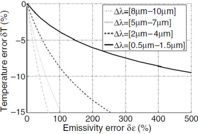
Fig. 1.16: Relative temperature error versus relative error on the emissivity at a given temperature

of 550 K. [TEY 07] ... 32

Fig. 1.17: Temperature measurement on a surface with gradients of emissivity, the infrared image on the left, the near-infrared image on the right. [ROT 06b]. ... 33

Fig. 2.1: Blackbody experimental set-up. ... 41

Fig. 2.2: Image acquired and the ROI with 1000 × 1000 pixels. ... 42

Fig. 2.3: Evolution of mean gray level of ROI as a function of exposure time for the given temperatures of 1223 K and 1253 K. ... 42

Fig. 2.4: Evolution of mean gray level of ROI as a function of temperature for the given exposures time of 7 ms and 3 ms. ... 43

Fig. 2.5: Radiometric calibration function identified on experimental data (cross points). ... 44

Fig. 2.6: Temperature errors of radiometric model. ... 44

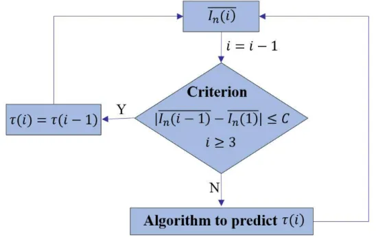
Fig. 2.7: Schematic diagram of the basic principle of the approach. ... 46

Fig. 2.8: Flow chart of the approach to maintain the image gray level constant. ... 47

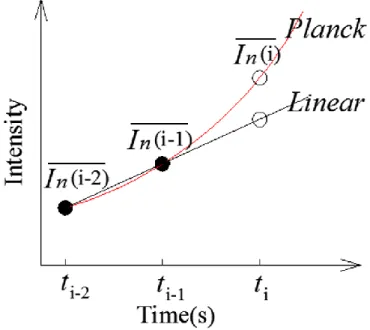
Fig 2.9: Principle of the specific law of exponential function and linear function. ... 49

Fig. 2.10: Simulated results of linear algorithm. ... 50

Fig. 2.11: Experimental results of linear algorithm. ... 50

Fig. 2.12: Simulated results of Planck’s algorithm. ... 51

Fig. 2.13: Experimental results of Planck’s algorithm. ... 51

Fig. 2.14: Experimental errors of linear algorithm and Planck’s algorithm. ... 52

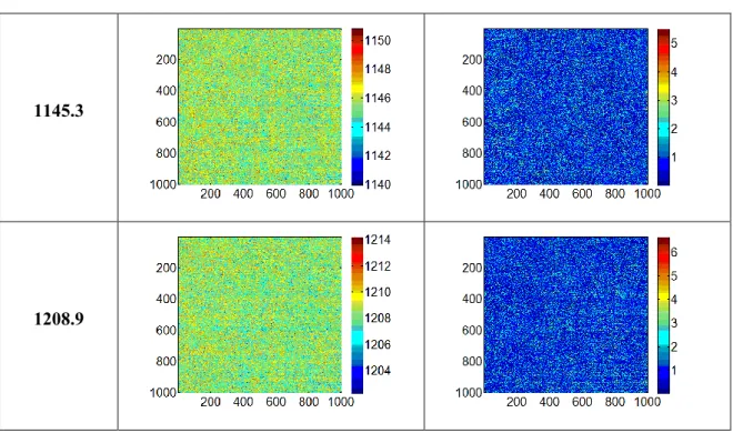
Fig. 3.1 Reconstructed thermals field and error fields from recorded images with mean gray level conservation (Planck’s algorithm). ... 59

Fig. 3.2: The mean temperature errors and standard deviations (error bars) of error fields at various temperatures of pyrometer ... 59

Fig. 3.3 Experimental set-up: the observed surface is located between the two induction heating coils. ... 60

Fig. 3.4: Acquired image of specimen surface under induction heating: Rectangle 1 is the ROI for exposure time adjustment; rectangles 2-1 and 2-2 are considered for the identification of the radiometric model; rectangle 3 is the area of thermal field reconstruction; rectangles 4-1 and 4-2 are considered for the validation of the reconstructed thermal field. ... 61

Fig. 3.5: Mean gray level of ROI 1 and exposure time evolves as the temperature measured by

pyrometer increases with/without exposure time adjustment. ... 62

Fig. 3.6: Some images acquired at various temperatures using a constant exposure time. ... 63

Fig. 3.7: Some images acquired at various temperatures with exposure time adjustment. ... 64

Fig. 3.8: Identification of the radiometric model parameters: rounds and crosses represents the mean gray level of areas 2-1 and 2-2 respectively as a function of the measured temperature by the pyrometer and thermocouple T2 respectively. ... 65

Fig. 3.9: Temperature errors of the radiometric model. ... 65

Fig. 3.10: Reconstructed thermal fields at different measured temperatures of T1. ... 67

Fig. 3.11: Temperature distribution along the longitudinal direction (see the black dotted line in Figure 3.10(a)) for different temperatures commands given to the induction heating device. ... 68

Fig. 3.12: Temperature error between the calculated temperatures and measured temperatures by thermocouple 1 (T1) and thermocouple 3 (T3). ... 68

Fig. 3.13: Experimental set-up under heating plate. ... 69

Fig. 3.14: Acquired image of a specimen surface when heated by induction thanks to the plate. Green square is the reference area for exposure time adjustment; blue rectangle 2 is the reference area for radiometric model identification by comparison to thermocouple T2; red rectangle 3 is the area of thermal field reconstruction; yellow areas 4-1 and 4-2 are chosen to validate the thermal field by comparison the thermocouple T1 measurement. ... 70

Fig. 3.15: Mean gray level of ROI 1 and exposure time evolves as the temperature of T2 increases with/without exposure time adjustment. ... 71

Fig. 3.16: Some images acquired at various temperatures of T2 at constant exposure time. ... 72

Fig. 3.17: Some images at various temperatures of T2 acquired with exposure time adjustment. ... 72

Fig. 3.18: Experimental data and radiometric model. ... 73

Fig. 3.19: Temperature errors of the radiometric model. ... 74

Fig. 3.20: Reconstructed thermal fields at various temperatures measured by T2. ... 75

Fig. 3.21: Temperature distribution along the white dotted line. ... 76

Fig. 3.22: Temperature error between the calculated temperatures and temperatures measured by thermocouple T1. ... 76

Fig. 4.2: Thermal loading procedure and an acquired image. ... 84

Fig. 4.3: Gray level and exposure time evolves with the increase of temperature with/without exposure time adjustment. ... 85

Fig. 4.4: Some images acquired at various temperatures of thermocouple at constant exposure time. 85 Fig. 4.5: Some images acquired at various temperatures of thermocouple with exposure time adjustment. ... 86

Fig. 4.6: Finite element in the reference image. ... 88

Fig. 4.7: Displacement fields (Unit: Pixel) along the direction of y axis. ... 89

Fig. 4.8: Fields of correlation errors (Unit: %). ... 90

Fig. 4.9: (a) Radiometric models based on different percents of pixels, and (b) magnified A region. . 92 Fig. 4.10: Effect of different percent of pixels on the temperature errors. ... 92

Fig. 4.11: The distribution of temperature errors for different percents of pixels. ... 93

Fig. 4.12: A tube with speckle is heated for twice. ... 94

Fig. 4.13: Relative errors of intensity based on 5% brightest and 5% darkest pixels between twice heating processes. ... 94

Fig. 4.14: An example of the thermal field reconstructed based on 20% of discrete known pixel temperatures using fifth order polynomial fitting method. ... 95

Fig. 4.15: Reconstructed thermal fields (Unit: K) of ROI 3. ... 97

Fig. 4.16: Distribution of 162000 discrete temperature errors of four thermal fields in Fig. 4.15. ... 97

Fig. 4.17: Mean discrete temperature errors of four thermal fields in Fig. 4.15. ... 97

Fig. 4.18: Thermal field (Unit: K) at the same coordinates as displacement fields shown in Fig. 4.7. 98 Fig. A1: Gray level of the blue rectangle 2-2 with 100 × 100 pixels. ... 105

Fig. A2: Effect of number of pixels along the direction of the blue hollow arrow on mean gray level. ... 106

Fig. B1: Gray level of the blue rectangle 2-2 with 100 × 100 pixels. ... 107

Fig. B2: Gray level variation along the direction of the blue hollow arrow (see Fig. B1) as a function of the number of pixel. ... 108

List of Tables

Table 2.1: Three parameters of radiometric model of the blackbody. ... 43

Table 2.2: The parameters of two cases to validate and compare two algorithms. ... 49

Table 3.1: Three parameters of radiometric model of steel specimen surface. ... 64

Table 3.2: Three parameters of radiometric model of titanium alloy specimen surface. ... 73

General introduction

Nowadays, experimental science is faced with major multi-physical challenges (particularly thermo-mechanical procedure) requiring the development of advanced test benches, multiplying the use of in-situ measurement techniques. Measurement of deformation and temperature is very important for thermo-mechanical procedures, such as mechanical tests at high temperature (fatigue, fracture, impact, et al.) and materials processing at high temperature (welding, forming, heating treatment, et al.). To measure deformation, many methods have been developed, e.g., classical strain gages, grid method, speckle interferometry, digital image correlation, etc. Digital image correlation appeared in the early 1980s has a major impact in the non-contact full field kinematic measurement of mechanics of materials and structures, which is still undergoing very spectacular developments. Common silicon-based cameras are used to perform digital image correlation. With the rapid development of cameras technology and personal computers’ computational abilities, this technique will become more widely used in various fields. To know the temperature, many techniques are also available, e.g., thermocouple, thermistor, resistance temperature detector, and infrared thermography, etc. Among these methods, infrared thermography is an advanced real-time non-contact, high-speed response and full field measurement technique. Generally, infrared thermography is performed using infrared cameras. If both kinematic and thermal fields can be simultaneously obtained by digital image correlation and infrared thermography, which can provide rich and relevant information on the thermo-mechanical procedures.

To simultaneously obtain kinematic and thermal fields, many researchers have made efforts on this topic. Many different methods are proposed to simultaneously obtain two fields. The commonly used method is to use two different imaging systems. The kinematic field is obtained by digital image correlation using the silicon-based camera, and the thermal field is obtained by infrared thermography using the infrared camera. Then a posteriori data processing is conducted to integrate the space and time associations of these two fields. Some researchers used silicon-based camera and infrared camera to observe two different surfaces of the specimen, respectively. Srinivasan et al. [SRI 12] studied the Lüders deformation in the welded mild steel during uniaxial tensile testing. In their experiment, one surface of the specimen with black coating is used to perform infrared thermography using infrared camera so as to obtain the thermal fields, and the other surface of the specimen sprayed with speckle is used to perform digital image correlation so as to obtain the kinematic fields. Some other researchers

tried to use two imaging systems to observe the kinematic and thermal fields on the same specimen surface. Bodelot et al. [BOD 09] used a “filter-mirror” (dichroic mirror) to separate the infrared radiation and visible radiation, and a silicon-based camera is used to detect the visible radiation while an infrared camera is used to detect the infrared radiation. Simultaneous observation of kinematic and thermal fields in the same zone at the microstructure scale of an AISI 346L austenitic stainless steel specimen during tensile test was performed. However, these methods have some problems which are difficult to be simultaneously addressed: (1) Two different imaging devices have different spatial resolution and acquisition rates. The exact same spatial and temporal coordinates of kinematic and thermal fields cannot be achieved no matter how well the posteriori data processing is done; (2) The digital image correlation and infrared thermography have conflicting requirements for the specimen surface. DIC needs a heterogeneous and contrasting texture on the specimen surface, which is tracked to perform the kinematic fields. But the IRT needs a homogeneous and constant emissivity on the surface, of which the temperature can be measured with little influence of emissivity variation; (3) the combination of these two imaging systems is expensive and uneasy. Complicated experimental set-up should be conducted to combine these two imaging systems by special expensive filters and other installations due to the different spectral ranges acquired by these two systems. Too much extra devices are not easy to be installed around the specimens in the tests, especially if the specimen has a complex motion trajectory. Taking into account the above disadvantages, a few researchers tried to obtain simultaneously kinematic and thermal fields using a single type of camera. Maynadier et al. [MAY 12] used a single infrared camera to obtain kinematic and thermal fields in order to capture localized transformation bands of shape memory alloy under tension. Using a sole set of infrared camera, both two fields decomposed over the same time and space discretization can be obtained. However, the infrared camera delivered rather poor fields due to its low resolution. Moreover, the infrared cameras are expensive and difficult to be used, which are mostly used in the laboratory research. Compared with infrared camera, silicon-based camera is cheaper, presents lower noise, possesses longer durability and has major advantage to deliver a far higher resolution, and it can be widely used for industrial applications. Orteu et al. [ORT 08] tried to use a single type of silicon-based camera (CCD camera) to measure both displacement and temperature fields. However, the preliminary exploration has been done. Some problems have not been solved. The problem that the digital image correlation and infrared thermography have conflicting requirements for the specimen surface has not been addressed. The temperature they obtained is just the apparent temperature (i.e., radiation intensity) and the true temperature fields cannot be obtained. In addition, there is another problem for silicon-based camera to be used for temperature measurement. In the near-infrared spectral range, a small temperature variation will lead to a large modification in the image gray level, which easily leads to poor quality images due to oversaturation and/or poor dynamic range of gray levels. The stable image gray level is the basis for both digital image correlation technique and near-infrared thermography technique. Especially for the digital image correlation, the image

correlation is based on the gray level conservation between reference image and deformed images. The variation of image gray level will introduce large errors.

The objective of this thesis is to measure simultaneously kinematic and thermal full fields using a single silicon-based camera. The problems mentioned above are intended to be addressed when a silicon-based camera is used.

In Chapter 2, an innovative technique is proposed to automatically adjust the exposure time of the camera to obtain kinematically and thermally exploitable images whatever the temperature evolution occurs on the surface of the observed object. Then, the accuracy and reliability of this technique are validated by blackbody heating experiment.

In Chapter 3, the technique proposed in chapter 2 is used in the realistic applications, and the reliability and accuracy of this technique are further validated. Two specimen heating experiments are conducted. The radiometric models of specimen surfaces are calibrated. Then, thermal fields on specimen surfaces are reconstructed based on radiometric models.

In Chapter 4, tube ballooning experiment is conducted, and both kinematic and thermal fields on the tube surface are intended to be obtained. Global digital image correlation is performed to obtain continuous kinematic field. An innovative method is proposed to calibrate an accurate radiometric model for heterogeneous specimen surface with different emissivity paints. This study offers a low-cost simplified technique for obtaining simultaneously kinematic and thermal fields.

Chapter 1

State of the art

This chapter contains three parts; it presents the kinematic field

measurements by digital image correlation, the thermal field

measurements by infrared thermography, and the current situations of

Contents

1.1 Measurement of kinematic fields ... 7

1.1.1 Introduction of digital image correlation ... 8 1.1.2 Measurement set-up for digital image correlation measurement... 11 1.1.3 Basic principles of digital image correlation computation ... 12

1.2 Measurement of thermal fields ... 16

1.2.1 Introduction of infrared thermography ... 17 1.2.2 Fundamentals of infrared thermography ... 18 1.2.3 Infrared thermometry ... 22 1.2.4 Infrared thermal imaging ... 25

1.3 Current status of coupling kinematic and thermal fields ... 26

1.3.1 Combination of two imaging systems ... 26 1.3.2 Single imaging device for both fields measurement... 30

Nowadays, many topics of mechanical science involve thermomechanical coupled phenomena: (1) Determination of complex constitutive model (shear bands, phase transformation, and so on); (2) Description and modeling of rupture (cracking, self-heating in fatigue, and so on); (3) Study of the manufacturing processes (modeling/development of the welding/forging, study of the cutting during milling, and so on). The analysis of these phenomena assumes the consideration of some kinematic and thermal quantities that the experimenter can attain in the form of displacements and temperatures. This raises a series of questions concerning the reliability of the measurements, the dimensions of the regions of interest and the non-disturbance of the phenomenon by the measurement itself.

The joint exploitation of these two quantities of interest allows better understanding, modeling and identifying the coupled phenomena. It is therefore necessary that the two quantities (thermal and kinematic) are measured on the same surface or the same regions of interest and at the same time. The first part of this chapter presents the kinematics field measurement. First a short general point of view is given prior to focus on the full field measurement by image correlation: the imaging set-up that it generally requires and the basic principles of how it works.

The second part of this chapter presents the thermal field measurement, and especially the most common technique for thermo-mechanical application: the middle-wave infrared thermography. The last part deals with the current status of coupling the two measurement methods and presents some recent works where the combination of both measuring techniques are used.

1.1

Measurement of kinematic fields

Measuring kinematic field consists in evaluating displacement or deformation on the surface of materials or structures subjected to various loading, across a large area of interest, but often with local resolution. Kinematic fields are commonly obtained using non-contact optical methods. By this way, the measurement of kinematic fields circumvents many issues:

(1) How to avoid the disturbance of the observed phenomena?

(2) How to obtain global information about the displacement of the observed surface? (3) How to detect local events (cracking, shear or strain localization, and so on)?

There are very important issues, which have been paid special attention in experimental mechanics and materials science. Indeed, some of the commonly used technologies for the displacement or deformation measurement are: (1) the finite difference of the rigid body displacement at the edge of the observed structure; (2) the use of glued strain gages.

In the first case, the experimenter uses the displacement measured by the testing machine itself or the relative displacements of two arms of an extensometer glued or clamped on particular points of the surface. Beyond the practical implementation problems that this entails, the information obtained is then averaged between the points whose movements are known. A local phenomenon can be totally ignored, and if it is detected, we will not be able to know its position and magnitude. In the second case, strain

gauge is a contact measurement method. However, it has some disadvantages. The gauge should be glued to the specimen surface. If a small specimen or soft material are considered, the additional stiffness and weight of the strain gauge will affect seriously the measurement results. Moreover, strain gauge measurement is a point measurement method, and the full field cannot be obtained. It is difficult to use this method for studying non-uniform deformation behaviors. Lastly, strain gauge has a limited measurement range. The large deformation will break the strain gauge resistance wire, so the measurement data cannot be obtained.

The optical measurement methods are non-contact full-field measurement methods, which can deal with the aforementioned issues. There are many kinds of optical measurement methods that permit to quantify displacements: (1) interferometry technique, such as holography interferometry, speckle interferometry, moire interferometry; (2) non-interferometric techniques, such as digital image correlation (DIC), particle image velocimetry (PIV).

Interferometric optical measurement methods measure the deformation by interpreting interferences. In the case of moire or speckle interferometry, the interferences are obtained by projecting a particular pattern (grid, line, or speckle) on the exact same pattern coating the imaged object. The superposition discrepancy reveals local displacements and creates figures that can be interpreted to quantify the displacements. The laser interferometry proceeds by recording the phase difference of the scattered light wave from the test object surface before and after deformation. It could be used to obtain spot measurements or field measurements thanks to a high-speed scanning. This technique usually needs a coherent light source, normally the laser. However, the interferometry measurements have high requirements for the external environment, which should be conducted in a vibration-isolated optical platform. Thus, these techniques are normally used in the laboratory, and are difficult to be used in industrial applications due to the complex environment.

Non-interferometric optical measurement methods measure the deformation of the object surface by comparing the gray intensity changes before and after deformation. Non-interferometric optical measurement methods only need a non-coherent light source, thus they are easier to be used than the interferometric optical measurement methods. DIC is a representative non-interferometric metrology, which has been widely used for the deformation measurement of solid materials [MCC 10][HIL 06].

1.1.1 Introduction of digital image correlation

The emergence and development of DIC is contributed by the rapid development of cameras technology and personal computers’ computational abilities.

Compared with the interferometric techniques, DIC presents some attractive advantages: (1) Simple experimental set-up

A single basic camera, such as a charge-coupled device (CCD) or a complementary metal-oxide-semiconductor (CMOS) is needed to record images of the object surface during its movement.

If the specimen surface has a natural texture, which has a random gray intensity distribution, the natural texture can be used as speckles to be easily tracked in DIC. If not, the surface can be prepared simply by spraying black and/or white paints as speckle.

(3) Strong environmental adaptability

The DIC technique does not need a laser source. White light source or natural light is enough for the measurement. Even if it is preferable that the illumination of the imaged scene stays constant all through the recording process, some lighting variation can be tolerated as long as the surface texture remains obvious. However, DIC can be used in complex work conditions, such as high temperature, high pressure, high-speed impact, vibration, et al. Thus it is very suitable for industrial applications. (4) Wide measurement range

DIC deals with digital images, thus these images can be acquired by various high-resolution digital acquisition devices, such as optical microscopy [SUN 97][PIT 02], laser scanning confocal microscope (LSCM) [BER 06][FRA 07], scanning electron microscopy (SEM) [KAN 05][WAN 06], transmission electron microscopy (TEM) [CAL 14], atomic force microscopy (AFM) [CHA 05][SUN 06], scanning tunneling microscope (STM), [VEN 98a][VEN 98b][VEN 98c], and satellites [SCA 62][LEP 07]. All these kinds of images can be analyzed by DIC to make microscale to macroscale displacement measurement.

The idea of DIC technique was first proposed in the early 1980s by Japanese I. Yamaguchi [YAM 81][YAM 81] and W.J. Peters and W.F. Ranson [PET 82] of the University of South Carolina in the United States. I. Yamaguchi investigated the behavior of the small object deformation by calculating the cross-correlation functions of speckle illumination intensities before and after the deformation. Peters and Ranson performed the iterative operations on the digital images of the object acquired before and after deformation. They calculated the correlation coefficient with the change of displacement and its derivative to find the extreme value of the correlation coefficient, thereby obtaining the corresponding displacement.

Many researchers did a lot of work on how to speed up the calculation and improve the calculation accuracy. Peters [PET 83] firstly applied DIC technique to measure the displacement of the rigid body. In the same year, Sutton et al. [SUT 83] improved the correlation search method, and used the combination of coarse correlation and fine correlation to improve the calculation speed. HE et al. [HE 84] studied the accuracy of the DIC technique and improved the theory of this measurement method. Sutton et al. [SUT 86][SUT 88] analyzed the measurement error caused by the subpixel recovery process, and proposed reasonable methods to deal with subpixel recovery. Bruck et al. [BRU 89] used the Newton-Raphson iterative algorithm based on binary cubic spline interpolation sub-pixel reconstruction to solve the DIC problem, which greatly improved the DIC method. Vendroux and Knauss [VEN 98] used a first-order derivative approximation to process the Hessian matrix, i.e. that the New-Raphson algorithm was replaced by Gauss-Newton algorithm, which improved the computational efficiency by removing the process of calculating the second-order gray level gradient while ensuring the calculation

accuracy. Borgefors et al. [BOR 01] proposed the hierarchical search method, which decomposed two images to be matched into a series of images whose size gradually decreases and the resolution gradually decreased. The matching of images was from the lowest resolution level, and then gradually backtrack the results, thereby increasing the calculation speed and usability of the method. Yoneyama and Morimoto [YON 03] replaced the gray speckle pattern in the DIC technique by color speckle pattern, which improved the accuracy of displacement and strain. Réthoré et al. [RET 07a][RET08] applied the extended finite element to DIC, thereby greatly improving calculation accuracy of the discontinuous behaviors, such as cracking. Since the emergence of DIC technique, there are still many outstanding scholars who contributed to this term. Thus, the DIC technique is still undergoing very spectacular developments.

In addition to improving calculation speed and accuracy, the practical applications of DIC technique is another important topic. Its applications mainly focus on the following three aspects. (1) Measuring the deformation properties and mechanical properties of various materials (such as metal, composite, polymer, wood, et al.) under mechanical loading and thermal loading. Zikn et al. [ZIK 95] firstly used DIC technique to investigate the mechanical properties of wood. Choi et al. [CHO 97] applied DIC technique to measure the deformation of concrete under compressive loading, and obtained the failure performance of concrete. Bastawros et al. [BAS 00] used DIC technique to obtain three stages deformation process of the aluminum alloy foam under compressive loading. Chevalier et al. [CHE 01] investigated the axial tensile tests of a kind of polymer by DIC.

(2) Based on the information of displacement and strain obtained by DIC technique, the various materials’ parameters can be calculated, such as elastic modulus, Poisson's ratio, thermal expansion coefficient, stress intensity factor, fracture toughness, et al. Zhang et al. [ZHA 02] studied the variation of Poisson's ratio of the arterial vessels with axial strain by DIC. Yoneyama [YON 06] and Réthoré [RET 05] used DIC technique to measure the stress intensity factor at the crack tip. Pan et al. [PAN 07] obtained the deformation information of film, so the thermal expansion coefficient of the film can be calculated.

(3) The full field deformation data of the object surface by DIC technique is used to perform theoretical analysis and numerical simulation [SAB 06][KNA 03][CHO 05]. Thus, the theory, simulation and experiments can be linked.

After years of development, DIC technique has expanded from the initial displacement analysis in metal testing to many other fields, such as biomedicine, civil engineering, aerospace, electronics, and so on. Meanwhile, with the appearance of the atomic force microscopy, transmission electron microscopy and scanning tunneling microscope, the DIC is widely used in microscopic observations. In the past few decades, DIC has shown its great potentiality. From the perspective of further development, DIC technique will inevitably be applied to a wider range of fields with the rapid development of computers and imaging devices.

1.1.2 Measurement set-up for digital image correlation measurement

Specimen preparation

The surface of the measured object must have a random gray intensity distribution. Generally, the random speckle pattern is used as a carrier of displacement information. Some examples of speckles are schematically shown in Fig. 1.1. An isotropic pattern guarantees that the displacement could be identified in every direction of the plane. High-contrast speckle patterns ensure that the gradient will be maximum. An example of the best pattern is shown in Fig. 1.1(d). Other three patterns are not good patterns to perform DIC. Some natural texture of the specimen surface, such as the grains on the metal surface or milling streaks, can be aleatory enough to be tracked by DIC. However, in most cases, artificial speckles are made by spraying black and/or white paints.

(a) Repetitive, anisotropic, high-contrast. (b) Non-repetitive, anisotropic, high-contrast.

(c) Non-repetitive, isotropic, low-contrast. (d) Non-repetitive, isotropic, high-contrast.

Image acquisition system

The general image acquisition system for performing DIC is schematically shown in Fig. 1.2. There are four main elements: (1) specimen with surface speckle; (2) silicon-based camera (CCD or CMOS); (3) computer for data acquisition; (4) white light source. The camera is placed with its optical axis normal to the specimen surface. The white light source is used to provide a good view of the specimen surface with high-contrast gray level intensity distribution. When the specimen is under loading, the camera simultaneously records the images. Then, a posteriori processing of the acquired images is performed to obtain the displacement fields by the computer. The strain fields can be inferred from the displacement fields.

Fig. 1.2: Typical optical image acquisition system [PAN 09].

1.1.3 Basic principles of digital image correlation computation

The basic principle of DIC is to select a reference sub-set with (2k+1) × (2k+1) pixels (k is the number of pixels) in the reference image f x y( , ) (i.e., image acquired before deformation), then to determine the corresponding subset location in the deformed image g( ,x y ) based on the gray level information of the subset. One can notice here that this justify why the surface pattern must not be repetitive, otherwise the determined solution might not be unique. Thus, the displacement and strain can be obtained based on the change of subset location and shape in the two images.

In order to reach this goal, correlation calculations are required. Firstly, a set of suitable variables to represent the displacement and deformation of the subset in the reference image and the deformed image should be found. Secondly, a mathematical criterion should be established to evaluate the correspondence degree of two subsets: one in the reference image, the other one eventually strained and displaced image. Finally, using an efficient search algorithm, the displacement and strain of subset can be obtained by iterative calculation.

Shape functions

As shown in Fig. 1.3, a point P(x0, y0) is in the reference image. To compute the displacement of

point P, a reference subset centered at point P(x0, y0) from the reference image is used to track its

corresponding location in the deformed image. The reason why a square subset, rather than an individual pixel, is selected for matching is that the subset comprising a wider variation in gray levels will distinguish itself from other subsets, and can therefore be more uniquely identified in the deformed image.

The subset centered at point P(x0, y0) moves to a location near point P'(x0', y0'). The displacement

of point P on the x and y axes is u and v, respectively. Thus,

0 0 0 0

x

x

u

y

y

v

   





  



(1.1)

Meanwhile, point Q(xi, yi) represents any point around the point P in the reference subset, positional relationship between point P and point Q is given as follows:

0 0 i i x x x y y y          (1.2)

where x and y is the distance between point P and point Q on the x and y axes, respectively. If the point Q in the reference subset moves to point Q'(xi', yi'), thus an equation can be given as follows:

i i Q i i Q

x

x

u

y

y

v

   





  



(1.3)

Generally, the material imaged in the reference subset allows translation, rotation and shear. Thus, the displacement of point Q on the x and y axes (uQ and vQ) can be given by the first-order displacement gradient of point P: Q Q

u

u

u

u

x

y

x

y

v

v

v

v

x

y

x

y







_{ }

_{ }

_



_

_





_

_

     









(1.4)

Substituting Eq. (1.4) into Eq. (1.3) yield

i i i i

u

u

x

x

u

x

y

x

y

v

v

y

y

v

x

y

x

y





       



_

_





_

_

       









(1.5)

Since point Q is any point in the subset, it is found from Eq. (1.5) that displacement of subset can be expressed by the displacement of the center point in the subset and its four derivatives (u_,v_, u

x   , u y   , v x   ,

v

y





).

Fig. 1.3: Schematically illustration of a reference square subset before deformation and a target subset

after deformation [PAN 10].

Correlation criterion

In order to evaluate the similarity degree between reference subset and deformed subsets, a correlation criterion should be given. To date, different correlation criteria are proposed. Generally, the correlation criteria involve two groups: Cross-correlation (CC) criteria and sum of squared differences (SSD) criteria. Three commonly used CC criteria are given as follows:

(1) Cross-correction (CC):



( , ) g( , )



k k CC k k

C

f x y

x y

 

 







(1.6) (2) Normalized cross-correction (NCC):





1 1 2 2 2 2 ( , ) g( , ) ( , ) ( , ) k k k k NCC k k k k k k k k f x y x y C f x y g x y             _ _{ }         







(1.7) (3) Zero-normalized cross-correction (NCC):



 











1 1 2 2 2 2 ( , ) g( , ) ( , ) g( , ) k k m m ZNCC k k k k k k m m k k k k f x y f x y g C f x y f x y g                   _{ }  _  _ _{  }       _{   }   







(1.8) where

_

_

2 1 ( , ) 2 1 k k k k fm f x y k    



and





2 1 g( , ) 2 1 k k m k k g x y k      



.

Three commonly used SSD criteria are given as follows: (1) Sum of squared differences (SSD):





2

( , ) g( ,

)

k k SSD k k

C

f x y

x y

 

 







(1.9) (2) Normalized sum of squared differences (NSSD):









2 1 1 2 2 2 2

( , )

g( , )

( , )

g( , )

k k NSSD k k k k k k k k k k

f x y

x y

C

f x y

x y

     









 







_



_











_

_

_

_{ }

_





_

_

_

_













(1.10)

(3) Zero-normalized sum of squared differences (ZNSSD):









1 1 2 2 2 2 ( , ) g( , ) ( , ) g( , ) k k m m ZNSSD k k k k k k m m k k k k f x y f x y g C f x y f x y g                  _  _  _   _{  }       _{   }   







(1.11)

The basic principles of these correlation criteria are the same. Here, the normalized cross-correlation (NCC) is used to be analyzed as an example. The definition of NCC is given as follows:





1 1 2 2 2 2 ( , ) g( , ) ( , , , , , , , ) ( , ) ( , ) k k k k k k k k k k k k f x y x y u u v v C x y u v x y x y f x y g x y                   _{   }           







(1.12)

where x, y are the coordinates of the center point in the subset; x', y' are the coordinates of any point in the subset and can be obtained by Eq. (1.5). When maximum value is achieved (i.e., C=1), the subset in the deformed image are correlated with the reference subset in the reference image.

In correlation calculation, an optimization algorithm is normally adopted to find the minimum value. Thus, a correlation factor S is introduced:





1 1 2 2 2 2 ( , ) g( , ) 1 1 ( , ) ( , ) k k k k k k k k k k k k f x y x y S C f x y g x y                _ _{ }         







(1.13)

It is clear from Eq. (1.13) that the smaller the S value, the greater the correlation between the two subset.

Search algorithm

A vector J is introduced to represent the displacement of subset, which is given as follows:

J

x y u v

, , , ,

u

,

u

,

v

,

v

x

y

x

y



   



 

_{   }







(1.14)

Ji (i = 1, 2, 3, 4, 5, 6) is used to represent the u, v,

u x   , u y   , v x   , v y 

 . Thus, the correlation calculation is to find the minimum of objective function

S J J J J J J

( , , , , , )

_{1 2 3 4 5 6} . It is obvious that the necessary condition for S to achieve the minimum value is that its first-order derivative is equal to zero.

0

i

S

J



_



(1.15)

For this optimization problem, there are many numerical methods, such as Newton-Raphson, etc. When the S achieves the minimum value, we can obtain the displacement and deformation of the subset from the Ji values.

The aforementioned processes are the basic principles of local image correlation method, in which a small region of interest (i.e., the aforementioned reference sub-set) is chosen to be treated, as shown in Fig. 1.3. The main limitation of the local method is that the process can induce large fluctuations from one image to the other (from speckle and the variation of lighting).

The global image correlation method is better than the local method to avoid the limitations of the local method mentioned above [HIL 12]. The global method relies on the entire image to determine the displacement field based on a mesh and shape functions [BES 06]. The basic principles of global method will be described in Chapter 4, in which the global image correlation method will be performed by Finite element in our study.

1.2

Measurement of thermal fields

Temperature measurement is an important topic in many fields, especially high temperature measurement in aerospace, materials, energy, metallurgy and other high-tech fields. To measure the temperature, many techniques are available, which can be classified into two categories: (1) contact measurement techniques, the sensor is sealed on the surface or embedded into the material like thermocouples [GEN 09][BLO 80], thermistors[KIM 11], resistance temperature detectors [BLA 15],

etc. These sensors are well known, cheap and robust, but they provide a point information. Moreover, they fatally cause a disturbance in the observed phenomenon; (2) contactless measurement methods, the sensor exploits the change in radiation from the surface due to thermal change of the observed object. It can be a single point measurement like for infrared pyrometers or multisite sensors like becoming real cameras (infrared thermography) [PER 17][WAN 11][AST 06], etc.

The following subsections focus on the infrared thermography as a method of full thermal field measurement. Firstly, a general introduction of the infrared thermography is given. Then a brief introduction of the notion of thermometry, and particularly to the infrared thermometry, is proposed.

1.2.1 Introduction of infrared thermography

Infrared thermography (IRT) is an advanced real-time, non-contact, high speed response and full field measurement technique, which transforms the thermal radiation, emitted by objects in the infrared wavelength of the electromagnetic spectrum, into an electronic video signal with a resolution depending on the physical size of each pixel and of the whole sensor. IRT has some advantages:

(1) Non-contact measurement

Due to the infrared radiation of object surface being measured, it is unnecessary to touch the objects and it will not interfere with the thermal balance of the object. Therefore, this technique is very suitable for measuring moving or dangerous objects.

(2) Full field measurement

IRT outputs the full field temperature distribution of object surface, which not only provides complete information, but also is visually intuitive. In the mechanics of materials, it is particularly relevant for the observation of localized phenomena like localized phase transformation, cracking or damaging.

(3) High-speed response

The response time of conventional temperature measurement techniques (such as thermocouple) is in seconds, while the response time of IRT is in milliseconds or even microseconds. Thus, IRT is relevant for the observation of transient phenomena.

Development of the use of infrared thermography

The IRT was firstly used in the military. In World War II, Germans used infrared imaging tubes as photoelectric conversion devices to develop night vision devices and infrared communication devices [LIS 11]. After World War II, many countries have conducted extensive researches on the use of IRT in the military field. In late 1950s Texas instruments and the US Military developed the first single element detectors, which allowed the scanning of scenes and produced line images. In the late 1960s infrared camera was commercialized and thermal imaging became accessible to a wider audience, and not only to the military [BAR 12]. As the technology advances and matures, the application of IRT has been expanded to other fields.

In the medical field, measuring the temperature of the human body can contribute to both disease diagnosis and treatment planning. For example, IRT can be used for the diagnosis of superficial human body tumors such as malignant melanoma [DI 2003]. IRT can provide real-time information for the surgeon to assist him in decision making in the heart surgery [Ruddok 2003]. IRT is used in many other medical applications, such as the diagnosing of diabetic neuropathy or vascular disorders [RIN 10], fever screening [NGU 10], dentistry and dermatology [HAN 04], et al.

In the industrial field, IRT is an effective predictive maintenance tool. For example, IRT can be used to detect abnormal temperature patterns, thereby indicating faulty connections [CHO 09]. IRT can also be used in other areas of the maintenance and process monitoring field, such as monitoring of deformation [BAD 11], fatigue damage [LUO 98][PAS 08][WAN 00], welding [MEO 04][KAF 11][LAH 11], nuclear product monitoring [BLA 89][ITA 04], aerospace maintenance [FAV 95][MEN 06], et al.

For civil engineering applications, the temperature measurement of the facade of buildings can provide important information to discover many hidden conditions. For example, IRT is used to detect where and how energy is leaking from a building envelope. Besides the detection of heat loss, it can also be used to discover other anomalies, such as water infiltration and moisture [BOM 78][LJU 94] . A wet mass in a wall with the differentiated thermal inertia can be discovered by IRT. IRT is used for sub-surface moisture detection in masonry structures [MAI 09] and for moisture mapping in ancient buildings [GRI 02].

The applications of IRT are not limited to medicine, maintenance and buildings. Nowadays, this technique has been applied to various fields.

1.2.2 Fundamentals of infrared thermography

Random movements of molecules and atoms exist in any object above absolute zero, which emits thermal radiation. The more intense the movement of molecules and atoms is, the greater the energy is. The infrared wavelength range is approximately 0.76-1000 μm, which is between visible light and microwaves in the electromagnetic spectrum, as shown in Fig. 1.4. Much of infrared range of the electromagnetic spectrum is difficult to be used in IRT due to the lack of permittivity of the atmosphere and optical set-up concerning these typical wavelengths. Fig. 1.5 shows the atmospheric transmittance for different wavelengths. It is clear that the usable parts of the infrared for IRT involves: (1) Near-infrared (NIR) from 0.76 μm to 1.7 μm; (2) Short-wavelength Near-infrared (SWIR) from 1.7 μm to 2.5 μm; (3) Mid-wavelength infrared (MWIR) from 3 μm to 5 μm; (4) Long-wavelength infrared (LWIR) from 8 μm to 14 μm. Infrared radiation has a strong temperature effect. The higher the temperature of the object is, the stronger the infrared radiation energy is. Therefore, the temperature of the object surface can be obtained by measuring the infrared radiation energy. This is the theoretical basis for IRT.

Fig. 1.4: Electromagnetic spectrum (wavelength λ in micrometers) [CEN 97].

Fig. 1.5: Atmospheric transmittance at one nautical mile, 15.5℃, 70% relative humidity and at sea level [USA 14].

In the early 1800s, the English physicist William Herschel discovered thermal radiation outside the deep red in the visible spectral ranges, and this invisible light called infrared. After the observation of the infrared, many great scientists, such as Max Planck, Ludwig Boltzmann, Gustav Kirchhoff, James Clerk Maxwell, Joseph Stefan, Macedonio Melloni, et al., have made great contributions to IRT. Nowadays, IRT has become a useful technique to obtain the full field temperature distribution on the object surface.

The blackbody is an idealized physical body that absorbs all incident electromagnetic radiation, regardless of frequency or angle of incidence. Thus, blackbody can be used as a standard for radiation energy and is widely used for the calibration of infrared devices. In reality, the absolute blackbody does not exist. In 1860, Kirchhoff opened a small hole in an isothermally closed cavity. When the light entered the cavity through the small hole, it was reflected multiple times in the cavity, and was quickly absorbed

and attenuated. Finally, only a very small proportion of the radiation could emit from the small hole, as schematically shown in Fig. 1.6. This is the artificial blackbody.

Fig. 1.6: Blackbody model [ROB 09].

The spectral characteristics of the blackbody are measured, and the curve of the spectral radiation emission as a function of wavelength is shown in Fig. 1.7. It can be seen from the figure that there is a maximum value corresponding to each temperature, and the blackbody radiation increases rapidly with the increase of temperature. The maximum value of the curve is also gradually moved to the short wave side with the increase of temperature.