Using Mental Transformation Strategies for Spatial Scaling: Evidence from a Discrimination Task
Wenke Möhringa, Nora S. Newcombea, and Andrea Frickb a Temple University
b University of Fribourg
NOTICE: This is the peer reviewed version of the following article:
Möhring, W., Newcombe, N. S., & Frick, A. (in press). Using mental transformation strategies for spatial scaling: Evicence from a discrimination task.
A definitive version is published in Journal of Experimental Psychology:
Learning, Memory, and Cognition, 42, 1473-1479. DOI: 10.1037/xlm0000240
This article may not exactly replicate the authoritative document that will be published in the APA journal. It is not the copy of record. Changes resulting from the publishing process, such as editing, corrections, structural
formatting, and other quality control mechanisms may not be reflected in this document. This article may be used for non-commercial purposes in accordance with the journal’s conditions.
Corresponding Address: [email protected]
Author Note
Wenke Möhring and Nora S. Newcombe, Department of Psychology, Temple University, USA; Andrea Frick, Department of Psychology, University of Fribourg, Switzerland.
This research was supported by research grants from the US National Science
Foundation #SBE-0541957 and SBE-1041707 and a Research Grant from the Swiss National Science Foundation # PP00P1_150486. We are grateful to Alexander Boone for his support
with the experimental set-up and Andrew Ciampa and Ashley Goodwin for their help with data collection. In addition, we thank Hagen Paschke and David Landy as well as two anonymous reviewers for helpful suggestions.
Correspondence concerning this article should be addressed to Wenke Möhring, who is now working at the University of Fribourg, Rue de Faucigny 2, 1700 Fribourg,
Switzerland.
Abstract
Spatial scaling, or an understanding of how distances in different-sized spaces relate to each other, is fundamental for many spatial tasks and relevant for success in numerous professions. Previous research suggests that adults use mental transformation strategies to mentally scale spatial input, as indicated by linear increases in response times and accuracies with larger scaling magnitudes. However, prior research did not account for possible difficulties in encoding spatial information within smaller spaces. Thus, the present study used a discrimination task in which we systematically pitted absolute size of the spaces against scaling magnitude. Adults (N = 48) were presented with two pictures, side-by-side on a computer display, each of which contained a target. Adults were asked to decide whether the targets were in the same position or not, by pressing one of two computer keys. In one condition (constant-large), one space was kept constant and large, whereas the size of the other space was variable and smaller. In another condition (constant-small), the constant space was constant and small, whereas the size of the other space was variable and larger. Irrespective of condition, adults’ discrimination performance (d-primes) and response times were linear functions of scaling magnitude, supporting the notion that analog imagery strategies are used in spatial scaling.
Using Mental Transformation Strategies for Spatial Scaling: Evidence from a Discrimination Task
In modern technological societies, humans have created helpful tools to function successfully in their spatial environments (e.g., navigation aids and global positioning systems). But even though cognitive challenges are decreased by these tools, they are not eliminated. Using such
devices still requires spatial thinking, as the distances have to be mapped from one space (e.g., map) onto another space of a different scale (e.g., physical environment). This ability, called spatial scaling, is an integral requirement for many spatial tasks and a prerequisite for success in many professions. Scaling is also associated with many mathematical tasks such as
understanding proportions and fractions (Boyer & Levine, 2012; Möhring, Newcombe, & Frick, 2015; Möhring, Newcombe, Levine, & Frick, 2015). This close relation to mathematics and other disciplines is underlined by a recent report of the committee of the
National Research Council (NRC, 2012), which identified scaling as an important and overarching theme for different science disciplines.
Previous studies have indicated that spatial scaling emerges early in life
(Huttenlocher, Newcombe, & Vasilyeva, 1999). Using a simple task, 3-year-olds were able to use spatial information provided in small maps to find a hidden object in a larger rectangular sandbox. Yet, other studies indicated that this ability develops considerably across preschool (Frick & Newcombe, 2012; Vasilyeva & Huttenlocher, 2004). Even adults often exhibit difficulties, especially when it comes to very small or very large scales that cannot be directly experienced. Such difficulties have been shown in children and adults, for various temporal and spatial magnitudes (e.g., for geologic time: Resnick, Shipley, Newcombe, Massey, & Wills, 2012; for sizes ranging from an atom to the solar system: Tretter, Jones, Andre, Negishi, & Minogue; 2006), as well as for numerical magnitudes (Landy, Silbert, & Goldin, 2013; Rips, 2013; Siegler & Opfer, 2003; Thompson & Opfer, 2010).
Given the importance of scaling and the need for creating helpful interventions, it is surprising that relatively little is known about the underlying cognitive processes. One
strategy for comparing spaces of different sizes may be to encode distances in one space in an absolute manner and map these absolute distances onto the second space. Such a strategy would work well within spaces that are very similar in size; however, for larger differences in size, accuracy would decrease. Furthermore, when using such an absolute strategy,
participants’ response times (RTs) should not be affected by scaling magnitude (i.e., the absolute degree of scaling).
Another strategy would be to encode relative distances (cf. Huttenlocher et al., 1999). For example, a target location can be encoded as being at a third of the distance between two landmarks. Such relative or proportional distances can be encoded regardless of the absolute size of a space. In this case, scaling magnitude should affect neither participants’ RTs nor their error rates.
A third possible strategy is to use mental transformation (cf. Vasilyeva &
Huttenlocher, 2004). Participants may mentally expand or shrink the size of one space to match the other. In mental imagery research, linearly increasing RT patterns have been taken as an index for the use of such analog mental transformation strategies. For example,
increasing RTs have been found as a function of angular difference between stimuli in mental rotation tasks (e.g., Shepard & Metzler, 1971), as a function of distance in image scanning tasks (Kosslyn, 1975), or as a function of size in object matching tasks (Bundesen & Larsen, 1975; Larsen & Bundesen, 1978). Such RT patterns suggest that participants performed mental transformations that were subject to similar physical constraints as real
transformations, in that larger transformations took more time. By analogy, if participants use mental transformations for spatial scaling, one could expect increasing RTs as a function of scaling magnitude, and more imprecise responses the more the stimuli have to be transformed
mentally (cf. Cooper & Shepard, 1975; Kosslyn, Ball, & Reiser, 1978; Kosslyn, Digirolamo, Thompson, & Alpert, 1998; for linear error patterns).
In fact, a recent study (Möhring, Newcombe, & Frick, 2014) yielded evidence that participants use such a mental transformation strategy for spatial scaling, by showing that participants’ RTs and errors increased linearly with increasing degree of scaling. Möhring and colleagues measured scaling performance using a child-friendly localization task on a touch screen. Preschoolers and adults were asked to encode the location of a target on a map and to point to the same location in a larger referent space. Maps had the same size as or were smaller than the referent space, and the sizes of the maps were varied systematically (ranging from 5.5 cm to 22 cm), so that participants had to scale distance information from the maps by a particular factor (ranging from 1 to 4) to match the size of the referent space (22 cm).
Even though this approach clearly measured scaling processes, a limitation was that scaling factor was confounded with map size in this experimental set-up. Visual encoding of the target locations might have also been harder for very small maps and this might have resulted in increasingly slower and less accurate responses. Thus, this impaired visual
encoding might have resulted in linearly increasing RT and error patterns, while in fact adults might have used a relative distance strategy. Presenting maps that were larger than the
referent space could have clarified this point. However, presenting a small referent space was not practicable in this touch-screen paradigm, as participants responded with their index finger, and given its size, the spatial distribution of target location would have been too close.
The aims of the present study were two-fold. First, we aimed to support previous findings using a novel experimental procedure. Typically, spatial scaling has been
investigated using localization tasks, in which participants see spatial information on a map and are asked to reproduce target locations in another (typically larger) referent space. However, such localization tasks might favor particular response strategies; therefore,
replicating previous results using a different paradigm would strengthen conclusions about underlying cognitive processes involved in scaling. In the present study, we presented adults with a discrimination task akin to the ones used in mental rotation research. Participants saw two identical but different-sized spaces simultaneously, each containing a target. They were asked to decide whether the target positions were the same or different in the two spaces, by pressing one of two computer keys, and we measured their RTs and discrimination
performance (d-primes). To decide whether the presented spaces matched or not, participants presumably needed to scale one of the spaces to match the size of the other in order to
compare them.
Second, we aimed to disentangle whether previous linear response patterns were due to impaired visual encoding of relational distances rather than mental transformation
processes. Therefore, we systematically pitted absolute size of the spaces against scaling magnitude. As in previous studies, we manipulated scaling magnitude by systematically varying the size of one space while holding the other one constant. In one condition, the size of the constant space was large (constant-large condition), whereas the variable spaces were the same or smaller (similar to Möhring et al., 2014). Therefore, the smallest of the variable spaces required the highest degree of scaling to compare it to the constant space (factor of 2.6), but target locations were also most difficult to encode. In another condition, the size of the constant space was the same or smaller than the variable spaces (constant-small
condition). In this condition, the largest of the variable spaces required the highest degree of scaling to match the constant space, but here visual encoding should not have posed a problem. Consequently, we expected concurrent response patterns for both conditions if participants used mental transformation strategies. That is, regardless of condition we expected participants to show increased RTs (positive RT slopes) and decreased d-primes (negative d-prime slopes) with increasing scaling magnitude. In contrast, if previous results
were merely due to impaired encoding of spatial information in small spaces, we expected a positive RT slope for the large condition, but a negative RT slope for the
constant-small condition (and a similar inverse slope pattern for d-primes).
Method Participants
Forty-eight adults were tested: 24 in the constant-large condition (Mage = 21.54 years; SD =
1.10, 13 females, 19 right-handed) and 24 in the constant-small condition (Mage = 23.65
years; SD = 3.95, 14 females, 24 right-handed). Participants were students who participated to earn credits for their psychology courses. All of them had normal or corrected-to-normal vision. Two additional participants were tested but excluded from the constant-small sample because their individual discrimination performance (mean d-prime) did not significantly differ from 0, suggesting that they responded randomly.
Stimuli
Stimuli were presented on a computer monitor (50.8 cm in diagonal). Each trial began with a fixation cross in the center of the screen. Participants were instructed to initiate test trials themselves by pressing the space bar on the keyboard, upon which the stimuli appeared. To keep stimuli comparable to those of previous studies (Möhring et al., 2014), we used the same pictures. In half of the test trials, adults saw two circular green spaces located side-by-side, each containing a target (i.e., a white egg with a black contour). Target locations varied in the horizontal dimension between two landmarks (see Figure 1). In the other half of the test trials, participants saw two rectangular green spaces, in which target locations varied in the horizontal and the vertical dimension. This allowed us to investigate whether the degrees of freedom in the target distribution (1D vs. 2D) affected discrimination performance (cf. Huttenlocher et al., 1999; Vasilyeva & Huttenlocher, 2004). The size of one space was kept constant, whereas the other space was varied by systematically decreasing (constant-large
condition) or increasing (constant-small condition) its size (for sizes and scaling magnitudes, see Table 1). To keep the average distance between the targets constant across the different-sized spaces, the positions of both spaces were centered on a fixed point in the middle of the left and right half of the screen.
Design
Participants were presented with 1D target distributions on half of the trials, and with 2D distributions on the other half. Within these target distributions, targets were presented in 15 different locations. In one third of the trials, targets were presented in the same position in both spaces (match trials); in another third, targets were off by 2 cm for the constant-large condition and 1 cm in the constant-small condition (easy mismatch trials); in the last third, targets were off by 1 cm in the constant-large condition and 0.5 cm in the constant-small condition (hard mismatch trials). These distances pertain to non-scaled trials – naturally, they were different for scaled trials, but proportionally equivalent across scaling magnitudes (i.e., 9% of the horizontal extent for easy mismatches and 4.5% for hard mismatches). For 1D target distributions, mismatch trials were created by moving the target locations in the variable spaces to the left or right; for 2D target distributions they were moved left, right, up, or down (on approximately the same number of trials).
Scaling magnitude was varied from 1 to 0.25 for the constant-large and from 1 to 0.375 for the constant-small condition (see Table 1). In the constant-large condition, we used an identical range of scaling magnitudes as in previous research for comparability reasons (cf. Möhring et al., 2014); however, this was not possible for the constant-small condition due to limited space on the computer monitor. Therefore, results presented in the following will focus on scaling magnitudes from 1 to 0.375 in both conditions. For the constant space in the constant-small condition, a medium size of 320 pixels (i.e., 9.29 cm) for the widths of
rectangles and the diameters of circles was chosen, due to space limitations and to ensure unimpaired visual encoding.
The within-participants variables of target distribution (1D, 2D), item type (match, easy mismatch, hard mismatch), scaling magnitude (1 to 0.375), and target location (15) were combined in a full factorial design, amounting to 540 trials (630 in the constant-large condition). Trials with 1D vs. 2D target distributions were blocked, and it was
counterbalanced between participants which distribution they saw first. All other within-participants variables were presented in random order. Additionally, we counterbalanced between participants whether they saw the variable space on the left or right side of the monitor, whether they had to press the F- or J-key to indicate a match, and whether the size of the constant space was large or small (constant space condition), in order not to confuse participants.
Procedure
Individual testing took place in a quiet laboratory room. Participants were seated at a table with the computer monitor approximately 50 cm in front of them. A keyboard was located in front of the monitor and prepared in a way that only the J-key, the F-key, and the space bar were accessible, whereas the rest was covered with orange cardboard. Participants were instructed that they will see two pictures on the monitor and that both pictures will contain an egg. Their task was to decide whether the eggs were at the same position within the pictures by pressing the assigned computer key (either J for “same” and F for “different”, or vice versa, depending on condition). The experiment was presented in two blocks (one per target distribution) and participants were allowed to rest a few minutes in between. At the beginning of each block there were six practice trials for the corresponding target distribution, in which participants were presented with three match and three mismatch trials of the scaling
negative feedback (e.g., a smiling or a frowning face). Before starting the test trials,
participants were reminded to work as accurately and quickly as possible. Participants had a maximum of 5 s to respond before test trials were timed out and repeated. No feedback was provided in the test trials. Discrimination performance (d-primes) and RTs were measured. The entire session took about 40-50 minutes.
Results
D-Primes
As is typical in discrimination experiments, we applied Signal Detection Theory and calculated d-primes as a measure of participants’ discrimination performance (Green & Swets, 1966). We computed false-alarm and hit rates per constant space, scaling magnitude, target distribution, and item type, and z-transformed them1. D-primes were calculated by subtracting these false-alarm rates from hit rates (Stanislaw & Todorov, 1999). A d-prime of 0 indicates equal rates of false alarms and hits, hence suggesting no discrimination at all, whereas higher d-primes indicate better discrimination performance.
To test whether scaling magnitude affected participants’ d-primes, we calculated an analysis of variance (ANOVA) with scaling magnitude, target distribution, and item type as within-participant variables, and constant space as a between-participants variable. The ANOVA revealed a significant effect of scaling magnitude, F(5, 230) = 9.72, p < .001, ηP2 =
.17. Polynomial contrast showed a significant linear trend, F(1, 46) = 26.48, p < .001, ηP2 =
.37, whereas all other polynomial contrasts (2nd to 5th order) were non-significant (all Fs < 2.73, ps > .1). Participants’ discrimination performance decreased the more they had to scale
1 In cases of extreme values of false-alarm and hit rates (either 0 or 1) that prevented the calculation of d-primes, we followed common practice and adjusted them (Macmillan & Kaplan, 1985; Stanislaw & Todorov, 1999). Rates of 0 were replaced with 0.5 / n, and rates of 1 were replaced with (n – 0.5) / n, with n being the total number of match or mismatch trials, which in our case was 15.
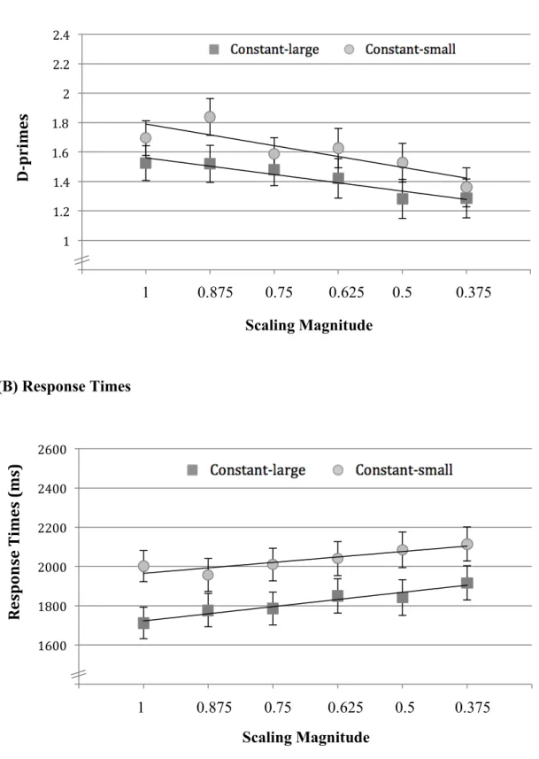
spatial information (see Figure 2A). However, there was no interaction of scaling magnitude and constant space condition, F(5, 230) = 1.04, p = .40, ηP2 = .02, suggesting that
participants’ discrimination was independent of whether the size of the constant space was large or small2.
The ANOVA also yielded a significant effect of item type, F(1, 46) = 568.68, p < .001, ηP2 = .93. Post hoc pairwise comparisons (Sidak corrected here and throughout)
revealed a higher discrimination for easy (M = 2.02, SE = 0.1) as opposed to hard mismatches (M = 1.02, SE = 0.07, p < .001). Another main effect was found for target distribution, F(1, 46) = 30.85, p < .001, ηP2 = .40, which was due to higher discrimination rates for 1D (M =
1.72, SE = 0.09) than 2D distributions (M = 1.32, SE = 0.08, p < .001). Furthermore, there was a significant 3-way interaction of target distribution, scaling magnitude, and item type, F(5, 230) = 2.74, p < .05, ηP2 = .06. To investigate this interaction, we looked at participants’
d-primes for target distributions and item types as a function of scaling magnitude and expressed this relation in terms of slopes. Slopes were defined as the change of participants’ d-primes per one step increase in scaling magnitude. For easy mismatch trials, slopes for 1D distributions (M = -.07) were higher than for 2D distributions (M = -.04), whereas the reverse was true for hard mismatch trials (1D: -.05 vs. 2D: -.09). However, slopes were consistently negative, indicating concurrent effects regardless of type or target distribution. There were no further effects (all Fs < 1.16, ps > .28). In an analogous ANOVA including sex, we found two 3-way interactions between sex, scaling magnitude, and target distribution, as well as
2 A significant effect of scaling magnitude on d-primes, F(6, 138) = 2.42, p < .05, ηP2 = .10, was also found for
the full data set of the constant-large condition, including the smallest map (scaling magnitude of 0.25). Again, polynomial contrast showed a significant linear trend only, F(1, 23) = 7.40, p < .05, ηP2 = .24 (with all other
sex, scaling magnitude, and constant space condition; however, slopes were negative in all cases, indicating that males and females responded concurrently.
Response Times
In a first step, we excluded RTs below 300 ms (0.0002% of the data), as is typical in discrimination tasks (cf. Ratcliff & Tuerlickx, 2002). RTs were then collapsed across the counterbalanced variables (response keys, location of the constant space, order of target distribution) and across the 15 target locations, because these variables were not central to the research question. Furthermore, preliminary analyses revealed no sex differences. Thus, sex was not considered in the following analyses. Similar to mental rotation research (e.g., Frick, Daum, Walser, & Mast, 2009), we focused on RTs of correctly solved trials (for analyses of the complete data set, see footnote3). On average, 14.1% of match trials were answered incorrectly, 21% of easy mismatch trials, and 51.9% of hard mismatch trials.
To test how scaling magnitude influenced participants’ RTs, an ANOVA was
calculated with the within-participant variables of scaling magnitude, target distribution, and item type, and the between-participants variable of constant space. The ANOVA yielded a significant effect of scaling magnitude, F(5, 230) = 14.86, p < .001, ηP2 = .24. Polynomial
3 To check whether this effect of scaling magnitude was limited to correctly solved trials, we ran a similar
ANOVA with the complete data. The ANOVA yielded a similar effect of scaling magnitude, F(5, 230) = 9.13, p
< .001, ηP2 = .17. Again, polynomial contrast showed a significant linear trend only, F(1, 46) = 21.71, p < .001,
ηP2 = .32, with all other contrasts being non-significant (all Fs < 3.07, ps > .08). However, there was also a
significant interaction between scaling magnitude and constant space, F(5, 230) = 5.07, p < .001, ηP2 = .10.
Separate ANOVAs for each constant space condition revealed significant effects of scaling magnitude for the constant-large condition, F(5, 115) = 3.42, p < .01, ηP2 = .13, as well as the constant-small condition, F(5, 115)
= 9.66, p < .001, ηP2 = .30. Again, these effects of scaling magnitude were best explained by linear functions in
the constant-large condition, F(1, 23) = 6.54, p < .05, ηP2 = .22, as well as in the constant-small condition, F(1,
contrast showed a significant linear trend, F(1, 46) = 52.54, p < .001, ηP2 = .53, whereas all
other polynomial contrasts (2nd to 5th order) were non-significant (all Fs < 1.10, ps > .32). Importantly, the interaction between scaling magnitude and constant space condition was non-significant, F(5, 230) = 1.71, p = .13, ηP2 = .04, indicating that scaling magnitude
affected participants’ RTs equally, regardless of whether the constant space was large or small. For both conditions, participants’ RTs increased with larger scaling magnitudes (see Figure 2B)4.
Additionally, the ANOVA revealed a significant main effect of item type, F(2, 92) = 16.09, p < .001, ηP2 = .26. Post hoc pairwise analyses indicated that participants’ RTs on
matches and easy mismatches did not differ (match: M = 1874, SE = 66; easy mismatch: M = 1846, SE = 54; p = .92), but on these trials RTs were significantly shorter than on hard mismatch trials (M = 2068, SE = 72, both ps < .01). Furthermore, item type interacted with constant space condition, F(2, 92) = 3.17, p < .05, ηP2 = .06, which was due to participants’
slower responses to match trials in the constant-small condition (M = 2041, SE = 94) compared to the constant-large condition (M = 1708, SE = 94, p < .01), with no significant differences for the other item types (ps > .21). Item type also interacted with scaling
magnitude, F(10, 460) = 4.47, p < .001, ηP2 = .09, and with scaling magnitude and constant
space condition, F(10, 460) = 2.87, p < .01, ηP2 = .06 (for detailed information, see Table 3).
To better understand these interactions, we again calculated RTs as a function of scaling magnitude and looked at the slopes (see Table 2). Even though on hard mismatches, slopes differed in size for the constant space conditions, slopes were positive in all conditions,
4 A significant effect of scaling magnitude on RTs, F(6, 138) = 7.52, p < .001, ηP2 = .25, was also found for the
full data set of the constant-large condition, including the smallest map (scaling magnitude of 0.25). Again, polynomial contrast showed a significant linear trend only, F(1, 23) = 33.75, p < .001, ηP2 = .60 (with all other
indicating that RTs increased with larger scaling magnitude regardless of constant space and item type.
The ANOVA also yielded a significant interaction of target distribution and scaling magnitude, F(5, 230) = 3.18, p < .01, ηP2 = .07, which was qualified by a significant
interaction of target distribution, scaling magnitude, and item type, F(10, 460) = 4.37, p < .001, ηP2 = .09. Separate analyses for each item type revealed no significant differences in
participants’ RTs when seeing matches or hard mismatches (all Fs < 1.66, ps > .14), but a significant interaction of target distribution and scaling magnitude for easy mismatches, F(5, 230) = 13.98, p < .001, ηP2 = .23. We again looked at slopes of participants’ RTs, which
indicated that on these easy mismatch trials, participants produced steeper slopes for 2D target distributions (103.85 ms per one step increase in scaling magnitude) than for 1D distributions (18.93 ms per step). However, slopes were positive in both cases, suggesting that participants’ RTs increased with larger scaling magnitude for both target distributions. There were no further effects (all Fs < 3.10, ps > .08).
Discussion
The present findings showed that adults’ RTs and d-primes were linear functions of scaling magnitude irrespective of the constant space condition. Regardless of whether the constant space was large or small, participants produced RTs that increased with larger scaling magnitude, whereas their discrimination performance decreased. In line with previous studies (Möhring et al., 2014), our findings indicate that adults use mental transformation strategies when scaling spatial information and rule out alternative explanations that increases in RTs and errors might have been merely due to an impaired encoding of spatial locations or relative distances.
Additionally, the present findings speak against a strategy of comparing absolute distances, because such a strategy would not result in a linear increase of RTs. Moreover, a
strategy focusing on absolute distances would lead to different error patterns with respect to the constant space conditions. Because targets displacements in mismatch trials decreased proportionally, the absolute target displacements were smaller in the constant-small
compared to the constant-large condition. Hence, if adults simply matched absolute distances between the presented spaces, they would have been more likely to indicate a match (produce more false-alarms and smaller d-primes) in the constant-small than the constant-large
condition. This response bias would have been indicated by an interaction between scaling magnitude and constant space condition. However, as our data revealed no such interaction, findings corroborate the notion that mental transformation strategies are used for spatial scaling, thus replicating Möhring and colleague’s results using a novel experimental procedure.
The present discrimination paradigm proved useful for investigating spatial scaling, and, in addition to replicating linear response patterns, the present results also support
findings that the complexity of the stimulus material influenced participants’ responses. Like in previous studies (Huttenlocher et al., 1999; Vasilyeva & Huttenlocher, 2004), participants performed more accurately when comparing pictures with 1D target distributions than 2D distributions. Participants’ responses also differed as a function of item type. Participants were slower and less accurate when responding to hard mismatches than to easy mismatches. The fact that participants produced a low percentage of correct responses for hard
mismatches suggests that these comparisons might have been too challenging for some of the participants. Nevertheless, participants showed positive RT slopes and negative d-prime slopes for every item type. Consequently, effects of scaling magnitude proved to be robust and independent of whether participants were responding to stimuli that were hard or easy to discriminate and of whether participants’ responses were fast or slow in general.
The finding that higher scaling magnitudes resulted in longer RTs and lower discrimination performance is consistent with findings on mental rotation, image scanning, and object matching (Bundesen & Larsen, 1975; Kosslyn, 1975; Larsen & Bundesen, 1978; Shepard & Metzler, 1971). The present finding that such a linear relation can also be
observed for spatial scaling suggests that a similar mental transformation mechanism is at play. This may also help to understand why even adults struggle with representing
magnitudes that are not directly observable (Landy et al., 2013; Resnick et al., 2012; Rips, 2013; Siegler & Opfer, 2003; Thompson & Opfer, 2010; Tretter et al., 2006). In such cases an analog mental representation cannot be generated and a transformation strategy might not be possible, because it may exceed the imaginable space in range or resolution. According to Kosslyn (1975) very small images are hard to evaluate, because they are constructed of an insufficient number of display units (like pixels on a TV), and very large images may “overflow” this imaginable space. Consequently, in such situations more abstract or formal rule-based strategies may be used.
Although our findings suggest that mental transformation strategies are used to scale spatial information, it is possible that children and adults rely on abstract thinking in specific situations (e.g., for unobservable scales) or use different strategies simultaneously. For example, it is likely that one may first use categorical information to roughly localize the target (e.g., the egg is in the upper right quadrant), and subsequently apply a mental
transformation strategy to determine the exact location (cf., the Category Adjustment Model; Huttenlocher, Hedges, & Duncan, 1991). Future studies should explore whether and how strategies are combined during spatial scaling.
Moreover, future research could help to clarify the role of attentional processes during spatial scaling. For instance, it may be that one’s attentional focus has to be shifted from a global to a more fine-grained level (or vice versa) when comparing spaces of different sizes.
Such a process of attentional re-focusing may be part of the scaling process and might also contribute to response times and error rates. Overall, more in-depth research on this topic is needed, and would have important practical implications, given the ubiquitous use of maps, models, and other symbolic representations in science, technology, engineering, and
References
Boyer, T. W., & Levine, S. C. (2012). Child proportional scaling: Is 1/3 = 2/6 = 3/9 = 4/12? Journal of Experimental Child Psychology, 111, 516-533.
Bundesen, C., & Larsen, A. (1975). Visual transformation of size. Journal of Experimental Psychology: Human Perception and Performance, 1, 214–220.
Cooper, L. A., & Shepard, R. N. (1975). Mental transformations in the identification of left and right hands. Journal of Experimental Psychology: Human Perception and Performance, 104, 48-56.
Frick, A., Daum, M. M., Walser, S., & Mast, F. W. (2009). Motor processes in children’s mental rotation. Journal of Cognition and Development, 10, 18–40.
Frick, A., & Newcombe, N. S. (2012). Getting the big picture: Development of spatial scaling abilities. Cognitive Development, 27, 270-282.
Green, D. M., & Swets, J. A. (1966). Signal detection theory and psychophysics. New York: Wiley.
Huttenlocher, J., Hedges, L. V., & Duncan, S. (1991). Categories and particulars: Prototype effects in estimating spatial location. Psychological Review, 98, 352–376.
Huttenlocher, J., Newcombe, N. S., & Vasilyeva, M. (1999). Spatial scaling in young children. Psychological Science, 10, 393-398.
Kosslyn, S. M. (1975). Information representation in visual images. Cognitive Psychology, 7, 341-370.
Kosslyn, S. M., Ball, T. M., & Reiser, B. J. (1978). Visual images preserve metric spatial information: Evidence from studies of image scanning. Journal of Experimental Psychology: Human Perception and Performance, 4, 47-60.
Kosslyn, S. M., DiGirolamo, Thompson, W. L., & Alpert, N M. (1998). Mental rotation of objects vs. hands: Neural mechanism revealed by positron emission tomography. Psychophysiology, 35, 151-161.
Landy, D., Silbert, N., & Goldin, A. (2013). Estimating Large Numbers. Cognitive Science, 37, 775-799.
Larsen, A., & Bundesen, C. (1978). Size scaling in visual pattern recognition. Journal of Experimental Psychology: Human Perception and Performance, 4, 1–20.
Macmillan, N. A., & Kaplan, H. L. (1985). Detection theory analysis of group data:
Estimating sensitivity from average hit and false-alarm rates. Psychological Bulletin, 98, 185-199.
Möhring, W., Newcombe, N. S., & Frick, A. (2014). Zooming in on spatial scaling: Preschool children and adults use mental transformations to scale spaces. Developmental Psychology, 50, 1614-1619.
Möhring, W., Newcombe, N. S., & Frick, A. (2015). The relation between spatial thinking and proportional reasoning in preschoolers. Journal of Experimental Child
Psychology, 132, 213-220.
Möhring, W., Newcombe, N.S., Levine, S.C., & Frick, A. (2015). Spatial proportional reasoning is associated with formal knowledge about fractions. Journal of Cognition and Development. doi: 10.1080/15248372.2014.996289
National Research Council (2012). A Framework for K-12 Science Education: Practices, Crosscutting Concepts, and Core Ideas. Committee on a Conceptual Framework for New K-12 Science Education Standards. Board on Science Education, Division of Behavioral and Social Sciences and Education. Washington, DC: The National Academies Press.
Ratcliff, R., & Tuerlinckx, F. (2002). Estimating parameters of the diffusion model: Approaches to dealing with contaminant reaction times and parameter variability. Psychonomic Bulletin & Review, 9, 438-481.
Resnick, I., Shipley, T. F., Newcombe, N. S., Massey, C., & Wills, T. W. (2012). Examining the representation and understanding of large magnitudes using the hierarchical alignment model of analogical reasoning. In N. Miyake, D. Peebles, & R. R. Cooper (Eds.), Proceedings of the 34th Annual Conference of the Cognitive Science Society. Austin, TX: Cognitive Science Society.
Rips, L. J. (2013). How many is a zillion? Sources of number distortion. Journal of Experimental Psychology: Learning, Memory, and Cognition, 39, 1257-1264. Shepard, R. N., & Metzler, J. (1971). Mental rotation of three-dimensional objects. Science,
171, 701-703.
Siegler, R. S., & Opfer, J. E. (2003). The development of numerical estimation evidence for multiple representations of numerical quantity. Psychological Science, 14, 237-250. Stanislaw, H., & Todorov, H. (1999). Calculation of signal detection theory measures.
Behavior Research Methods, Instruments, & Computers, 31, 137-149.
Thompson, C. A., & Opfer, J. E. (2010). How 15 hundred is like 15 cherries: Effect of progressive alignment on representational changes in numerical cognition. Child Development, 81, 1768-1786.
Tretter, T. R., Jones, M. G., Andre, T., Negishi, A., & Minogue, J. (2006). Conceptual Boundaries and Distances: Students’ and Experts’Concepts of the Scale of Scientific Phenomena. Journal of Research in Science Teaching, 43, 282-319.
Vasilyeva, M., & Huttenlocher, J. (2004). Early development of scaling ability. Developmental Psychology, 40, 682-690.
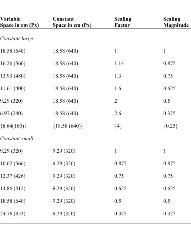
Table 1. Sizes of the stimuli (width of rectangles and diameters of circles), in cm (and Pixel) and the corresponding scaling factors and magnitudes used in the large and constant-small conditions.
Variable Constant Scaling Scaling
Space in cm (Px) Space in cm (Px) Factor Magnitude
Constant-large 18.58 (640) 18.58 (640) 1 1 16.26 (560) 18.58 (640) 1.14 0.875 13.93 (480) 18.58 (640) 1.3 0.75 11.61 (400) 18.58 (640) 1.6 0.625 9.29 (320) 18.58 (640) 2 0.5 6.97 (240) 18.58 (640) 2.6 0.375 {8.64(160)} {18.58 (640)} {4} {0.25} Constant-small 9.29 (320) 9.29 (320) 1 1 10.62 (366) 9.29 (320) 0.875 0.875 12.37 (426) 9.29 (320) 0.75 0.75 14.86 (512) 9.29 (320) 0.625 0.625 18.58 (640) 9.29 (320) 0.5 0.5 24.76 (853) 9.29 (320) 0.375 0.375
Note. Scaling factor is the ratio constant/variable space, and scaling magnitude describes the degree of scaling regardless of direction.
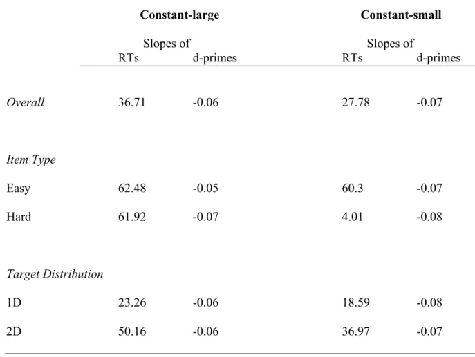
Table 2. Slopes of RTs (in ms) and d-primes as a function of scaling magnitude for each constant space condition, item type, and target distribution.
Constant-large Constant-small Slopes of Slopes of RTs d-primes RTs d-primes Overall 36.71 -0.06 27.78 -0.07 Item Type Easy 62.48 -0.05 60.3 -0.07 Hard 61.92 -0.07 4.01 -0.08 Target Distribution 1D 23.26 -0.06 18.59 -0.08 2D 50.16 -0.06 36.97 -0.07
Note. Slopes were defined as change in RTs or d-primes per one step increase in scaling magnitude (ranging from 1 to 0.375). Thus, in case of RTs, a positive slope indicates an increase in RTs, and thus, slower responses with larger scaling magnitudes. In case of d-primes, a negative slope indicates a decrease in d-d-primes, and thus poorer discrimination performance with larger scaling magnitudes.
Runni ng he ad : M E N T A L T RA N S F O RM A T IO N S F O R S CA L IN G T abl e 3. S ta ti st ic al va lue s of the e ff ec t of s ca li ng m agni tude in t he a na lys es of va ri anc e f or a dul ts ’ re spons e t im es a nd d -pri m es . M ai n e ffe ct of Li n ear c on tr as t In te rac ti on b etw ee n s cal in g sc al in g magn itu d e magn itu d e an d c on stan t s p ac e c on d F ηP 2 F ηP 2 F ηP 2 O ve ral l RT 14. 86 ** * 0.2 4 52 .54 *** 0.53 1. 71 ns 0.04 d-pri m es 9. 72 *** 0.1 7 26. 48 *** 0.37 1. 04 ns 0.0 2 T ype RT e as y 29 .4 3*** 0. 40 90. 69 *** 0.6 6 1.4 8 ns 0.03 RT har d 2.9 3* 0.06 12.00 ** 0.21 2.5 5* 0.05 d-pri m e eas y 5. 76 *** 0.1 1 13 .8 8** 0.2 3 0.72 ns 0.02 d-pri m e har d 9. 83 *** 0.1 8 34. 83 *** 0.4 3 1. 29 ns 0.03 * p < .05, ** p < .01, *** p < .001 .
Figure Captions
Figure 1. Examples of matching and mismatching stimulus pairs for the constant-large and constant-small conditions (presented with either 1D or 2D target distributions) for the scaling magnitudes 1, 1.3 and 2.6. Note that the targets were presented in white on green fields in the experiment.
Figure 2. Participants’ d-primes (A) and response times (B) as a function of scaling magnitude in the constant-large and constant-small conditions.
Figure 1.
Constant-large Constant-small
Item type: match; Scaling magnitude: 1
Item type: easy mismatch; Scaling magnitude: 1.3
Item type: hard mismatch; Scaling magnitude: 2.6
Constant Space Variable Space
Figure 2. (A) d-Primes (B) Response Times 0.8$ 1$ 1.2$ 1.4$ 1.6$ 1.8$ 2$ 2.2$ 2.4$ 0$ 1$ 2$ 3$ 4$ 5$ 6$ 7$ D "p ri m es) 1400$ 1600$ 1800$ 2000$ 2200$ 2400$ 2600$ 0$ 1$ 2$ 3$ 4$ 5$ 6$ 7$ R esp on se )T im es) (m s) ) 1 0.875 0.75 0.625 0.5 0.375 1 0.875 0.75 0.625 0.5 0.375 Scaling Magnitude Scaling Magnitude