HAL Id: lirmm-02991230
https://hal-lirmm.ccsd.cnrs.fr/lirmm-02991230
Submitted on 5 Nov 2020
HAL is a multi-disciplinary open access
archive for the deposit and dissemination of
sci-entific research documents, whether they are
pub-lished or not. The documents may come from
teaching and research institutions in France or
abroad, or from public or private research centers.
L’archive ouverte pluridisciplinaire HAL, est
destinée au dépôt et à la diffusion de documents
scientifiques de niveau recherche, publiés ou non,
émanant des établissements d’enseignement et de
recherche français ou étrangers, des laboratoires
publics ou privés.
Distributed under a Creative Commons Attribution| 4.0 International License
Parameterizations of Vertex Cover Admit a Polynomial
Kernel
Marin Bougeret, Bart Jansen, Ignasi Sau Valls
To cite this version:
Marin Bougeret, Bart Jansen, Ignasi Sau Valls. Bridge-Depth Characterizes Which Structural
Pa-rameterizations of Vertex Cover Admit a Polynomial Kernel. 47th International Colloquium on
Au-tomata, Languages, and Programming (ICALP), Jul 2020, Saarbrücken, Germany. pp.16:1–16:19,
�10.4230/LIPIcs.ICALP.2020.16�. �lirmm-02991230�
Parameterizations of Vertex Cover Admit a
Polynomial Kernel
Marin Bougeret
LIRMM, Université de Montpellier, CNRS, France http://www.lirmm.fr/~bougeret/
Bart M. P. Jansen
Eindhoven University of Technology, The Netherlands [email protected]
Ignasi Sau
LIRMM, Université de Montpellier, CNRS, France [email protected]
Abstract
We study the kernelization complexity of structural parameterizations of the Vertex Cover problem. Here, the goal is to find a polynomial-time preprocessing algorithm that can reduce any instance (G, k) of the Vertex Cover problem to an equivalent one, whose size is polynomial in the size of a pre-determined complexity parameter of G. A long line of previous research deals with parameterizations based on the number of vertex deletions needed to reduce G to a member of a simple graph class F , such as forests, graphs of bounded tree-depth, and graphs of maximum degree two. We set out to find the most general graph classes F for which Vertex Cover parameterized by the vertex-deletion distance of the input graph to F , admits a polynomial kernelization. We give a complete characterization of the minor-closed graph families F for which such a kernelization exists. We introduce a new graph parameter called bridge-depth, and prove that a polynomial kernelization exists if and only if F has bounded bridge-depth. The proof is based on an interesting connection between bridge-depth and the size of minimal blocking sets in graphs, which are vertex sets whose removal decreases the independence number.
2012 ACM Subject Classification Theory of computation → Graph algorithms analysis; Theory of computation → Parameterized complexity and exact algorithms
Keywords and phrases vertex cover, parameterized complexity, polynomial kernel, structural pa-rameterization, bridge-depth
Digital Object Identifier 10.4230/LIPIcs.ICALP.2020.16
Category Track A: Algorithms, Complexity and Games
Related Version The full version of this paper is permanently available at https://arxiv.org/abs/ 2004.12865.
Funding Bart M. P. Jansen: This project has received funding from the European Research Council
(ERC) under the European Union’s Horizon 2020 research and innovation programme (grant agreement No 803421, ReduceSearch).
Ignasi Sau: Supported by French projects DEMOGRAPH (ANR-16-CE40-0028) and ESIGMA
(ANR-17-CE23-0010).
1
Introduction
Background and motivation. The NP-complete Vertex Cover problem is one of the
most prominent problems in the field of kernelization [3, 8, 13, 16, 26], which investigates provably efficient and effective preprocessing for parameterized problems. A parameterized
problem is a decision problem in which a positive integer k, called the parameter, is associated
with every instance x. A kernelization for a parameterized problem is a polynomial-time algorithm that reduces any parameterized instance (x, k) to an equivalent instance (x0, k0) of the same problem whose size is bounded by f (k) for some function f , which is the size of the kernelization. Hence a kernelization guarantees that instances which are large compared to their parameter, can be efficiently reduced without changing their answer. Of particular interest are polynomial kernelizations, whose size bound f is polynomial.
An instance (G, k) of Vertex Cover asks whether the undirected graph G has a vertex set S of size at most k that contains at least one endpoint of every edge. Using the classic Nemhauser-Trotter theorem [28], one can reduce (G, k) in polynomial time to an instance (G0, k0) with the same answer, such that |V (G0)| ≤ 2k. Hence when using the size of the desired solution as the parameter, Vertex Cover has a kernelization that reduces to instances of 2k vertices, which can be encoded in O(k2) bits. While the bitsize of this kernelization is known to be essentially optimal [10] assuming the established conjecture NP 6⊆ coNP/poly, this result does not guarantee any effect of the preprocessing for instances whose solution has size at least |V (G)|/2. In particular, it does not promise any size reduction when G is simply a path.
To be able to give better preprocessing guarantees, one can use structural parameters which take on smaller values than the size of a minimum vertex cover, a quantity henceforth called the vertex cover number. Such structural parameterizations can conveniently be described in terms of the vertex-deletion distance to certain graph families F . Note that the vertex cover number vc(G) of G can be defined as the minimum number of vertex deletions needed to reduce G to an edgeless graph. Hence this number will always be at least as large as the feedback vertex number fvs(G) of G, which is the vertex-deletion distance of G to a forest. In 2011, it was shown that Vertex Cover even admits a polynomial kernelization when parameterized by the feedback vertex number [21, 22]. This triggered a long line of follow-up research, which aimed to find the most general graph families F such that Vertex Cover admits a polynomial kernelization when parameterized by vertex-deletion distance to F . Polynomial kernelizations were obtained for the families F of graphs of maximum degree two [27], of graphs of constant tree-depth [5, 23], of the pseudo-forests where each connected component has at most one cycle [17], and for d-quasi-forests in which each connected component has a feedback vertex set of size at most d ∈ O(1) [18]. Note that all these target graph classes are closed under taking minors. Using randomized
algorithms with a small error probability, polynomial kernelizations are also known for several
parameterizations by vertex-deletion distance to graph classes that are not minor-closed, such as Kőnig graphs [25], bipartite graphs [25], and parameterizations based on the linear-programming relaxation of Vertex Cover [19, 24]. On the negative side, it is known that Vertex Cover parameterized by the vertex-deletion distance to a graph of treewidth two [9] does not have a polynomial kernel, unless NP ⊆ coNP/poly. This long line of research into kernelization for structural parameterizations raises the following question:
How can we characterize the graph families F for which Vertex Cover parameterized by vertex-deletion distance to F admits a polynomial kernel?
Our results. We introduce a new graph parameter that we call bridge-depth. It has a recursive definition similar to that of tree-depth [30] (full definitions follow in Section 3), but deals with bridges in a special way. A graph without vertices has bridge-depth zero. The bridge-depth bd(G) of a disconnected graph G is simply the maximum bridge-depth of its connected components. The bridge-depth of a connected nonempty graph G is defined as follows. Let Gcbdenote the graph obtained from G by contracting each edge that is a bridge in G; the order does not matter. Then bd(G) := 1 + minv∈V (Gcb)bd(Gcb\ v). Intuitively, the bridge-depth of G is given by the depth of an elimination process [6] that reduces G to the empty graph. One step consists of contracting all bridges and removing a vertex; each of the remaining connected components is then recursively eliminated in parallel. From this definition, it is not difficult to see that bd(G) is at least as large as the tree-width of G, but never larger than the tree-depth or feedback vertex number of G. In particular, any forest has bridge-depth one.
Using the notion of bridge-depth, we characterize the minor-closed families F for which Vertex Cover parameterized by vertex-deletion distance to F admits a polynomial kernel.
ITheorem 1.1. Let F be a minor-closed family of graphs, and assume NP 6⊆ coNP/poly. Vertex Cover parameterized by vertex-deletion distance to F has a polynomial kernelization if and only if F has bounded bridge-depth.
Theorem 1.1 gives a clean and unified explanation for all the minor-closed families F that were previously considered individually [5, 17, 18, 22, 27], and generalizes these results as far as possible. To the best of our knowledge, Theorem 1.1 captures all known (deterministic) kernelizations for structural parameterizations of Vertex Cover. (There are randomized kernelizations [19, 24, 25] which apply for distance to classes F that are not minor-closed, such as bipartite graphs.) For example, we capture the case of F being a forest [22] since forests have bridge-depth one, and the case of F being graphs of constant tree-depth [5, 23] since bridge-depth does not exceed tree-depth. In this sense, bridge-depth can be seen as the ultimate common generalization of feedback vertex number and tree-depth (which are incomparable parameters) in the context of polynomial kernels for Vertex Cover.
We consider it one of our main contributions to identify the graph parameter bridge-depth as the right way to capture the kernelization complexity of Vertex Cover parameterizations.
Techniques. To describe our techniques, we introduce some terminology. Let α(G) denote the independence number of graph G, i.e., the maximum size of a set of pairwise nonadjacent vertices. A blocking set in a graph G is a vertex set Y ⊆ V (G) such that α(G \ Y ) < α(G). Hence if Y is a blocking set, then every maximum independent set in G contains a vertex from Y . Earlier kernelizations for Vertex Cover parameterized by distance to a graph class F , starting with the work of Jansen and Bodlaender [22], all rely, either implicitly or explicitly, on having upper-bounds on the size of (inclusion-)minimal blocking sets for graphs in F [5,17,18,22,27]. For example, it is known that minimal blocking sets in a bipartite graph have size at most two [18, Cor. 11], while minimal blocking sets in graphs of tree-depth c have size at most 2c [5, Lemma 1]. Similarly, all the existing superpolynomial kernelization
lower bounds for parameterizations by distance to F , rely on F having minimal blocking sets of arbitrarily large size. Indeed, if F is closed under disjoint union and has arbitrarily large blocking sets, it is easy to prove a superpolynomial lower bound (cf. [19, Thm. 1]).
Since all positive cases for kernelization are when minimal blocking sets of graphs in F have bounded size, while one easily obtains lower bounds when the size of minimal blocking sets of graphs in F is unbounded, the question rises whether a bound on the size of minimal
blocking sets is a necessary and sufficient condition for the existence of polynomial kernels. To our initial surprise, we show that for minor-closed families F , this is indeed the case: the purely structural property of having bounded-size minimal blocking sets can always be leveraged into preprocessing algorithms.
For an insight into our techniques, consider an instance (G, k) of Vertex Cover, together with a vertex set X ⊆ V (G) such that G \ X ∈ F for some minor-closed family F that has bounded-size minimal blocking sets. The goal of the kernelization is then to reduce to an equivalent instance of size |X|O(1) in polynomial time. Using ideas of the previous kernelizations [5,22], it is quite simple to reduce the number of connected components of G \ X to size |X|O(1). To obtain a polynomial kernel, the challenge is therefore to bound the size of each such component C of G \ X to |X|O(1), so that the overall instance size becomes polynomial in |X|. However, the non-existence of large minimal blocking sets does not seem to offer any handle for reducing the size of individual components of G \ X. The route to the kernelization therefore goes via the detour of bridge-depth. We prove the following relation between the sizes of minimal blocking sets and bridge-depth.
ITheorem 1.2. Let F be a minor-closed family of graphs. Then F has bounded bridge-depth if and only if the size of minimal blocking sets of graphs in F is bounded.
Using this equivalence, we can exploit the fact that all minimal blocking sets of F are of bounded size, through the fact that the bridge-depth of G \ X ∈ F is small. This means that there is a bounded-depth elimination process to reduce G \ X to the empty graph. We use this bounded-depth process in a technical kernelization algorithm following a recursive scheme, inspired by the earlier kernelization for the parameterization by distance to bounded tree-depth [5].
Let us now discuss the ideas behind the equivalence of Theorem 1.2. We prove that the bridge-depth of graphs in a minor-closed family F is upper-bounded in terms of the maximum size of minimal blocking sets for graphs in F , by exploiting the Erdős-Pósa property in an interesting way. We analyze an elementary graph structure called necklace of length t, which is essentially the multigraph formed by a path of t double-edges. If a simple graph G ∈ F contains a necklace of length t as a minor, then there is a minor G0 of G (which therefore also belongs to F ) that has a minimal blocking set of size Ω(t). Hence to show that bridge-depth is upper-bounded in terms of the size of minimal blocking sets of graphs in F , it suffices to show that bridge-depth is upper-bounded by the maximum length of a necklace minor of graphs in F . Since the definition of bridge-depth allows for the contraction of all bridges in a single step, it suffices to consider bridgeless graphs. Then we argue that in a bridgeless graph, any pair of maximum-length necklace minor models intersects at a vertex (cf. Lemma 4.6). By the Erdős-Pósa property, this implies that there is a constant-size vertex set that hits all maximum-length necklace minor models, and whose removal therefore strictly decreases the maximum length of a necklace minor. If the length of necklace minor models is bounded, then after a bounded number of steps of this process (interleaved with contracting all bridges) we reduce the maximum length of necklace minor models to zero, which is equivalent to breaking all cycles of the graph. At that point, the bridge-depth is one by definition, and we have obtained the desired upper-bound on the bridge-depth in terms of the length of the longest necklace minor, and therefore blocking set size.
For the other direction of Theorem 1.2, we prove (cf. Theorem 5.4) the tight bound that a minimal blocking set in a graph G has size at most 2bd(G). We use induction to prove this statement, together with an analysis of the structure of a tree of bridges whose removal decreases the bridge-depth. The fact that bipartite graphs have minimal blocking sets of size at most two, allows for an elegant induction step.
Related work. In a recent paper, Hols, Kratsch, and Pieterse [19] also analyze the role of blocking sets in the existence of polynomial kernels for structural parameterizations of Vertex Cover. Note that our paper is independent from, and orthogonal to [19]: we consider the setting of deterministic kernelization algorithms for parameterizations to
minor-closed families F , and obtain an exact characterization of which F allow for a polynomial
kernelization. Hols et al. [19] consider hereditary families F and give kernelizations for several such parameterizations, without arriving at a complete characterization. Some of the randomized kernelizations they provide do not fit into our framework, but all the deterministic kernelizations they present are captured by Theorem 1.1. Another contribution of [19] is to prove that there is a class F with minimal blocking sets of size one where Vertex Cover cannot be solved in polynomial time. In particular, there is no polynomial kernel parameterized by the distance to this family F , and thus bounded minimal blocking set size is not sufficient to get a polynomial kernel. This implies that our minor-closed assumption of Theorem 1.1 cannot be dropped.
We refer to the survey by Fellows et al. [13] for an overview of classic results and new research lines concerning kernelization for Vertex Cover. Additional relevant work includes the work by Kratsch [24] on a randomized polynomial kernel for a parameterization related to the difference between twice the cost of the linear-programming relaxation of Vertex Cover and the size of a maximum matching.
Organization. Preliminaries on graphs and complexity are presented in Section 2. Section 3 introduces bridge-depth and its properties. In Section 4 we prove one direction of Theorem 1.2, showing that large bridge-depth implies the existence of large minimal blocking sets. In Section 5 we handle the other direction, proving a tight upper-bound on the size of minimal blocking sets in terms of the bridge-depth. We discuss the kernelization algorithm exploiting bridge-depth in Section 6, with the technical content being available in the full version of the article [4] due to space limitations. We conclude the article in Section 7. The proofs of the results marked with “(?)” have been also deferred to the full version [4].
2
Preliminaries
Graphs. We use standard graph-theoretic notation, and we refer the reader to Diestel [11] for any undefined terms. All graphs we consider are finite and undirected. Graphs are simple, unless specifically stated otherwise. A graph G has vertex set V (G) and edge set E(G). Given a graph G and a subset S ⊆ V (G), we say that S is connected if G[S] is connected, and we use the shorthand G \ S to denote G[V (G) \ S]. For a single vertex v ∈ V (G), we use G \ v as a shorthand for G \ {v}. Similarly, for a set of edges T ⊆ E(G) we denote by G \ T the graph on vertex set V (G) with edge set E(G) \ T . A cycle on three vertices is called a triangle. For a positive integer i, we denote by [i] the set of all integers j such that 1 ≤ j ≤ i. Given v ∈ V (G), we denote NG(v) = {u | {u, v} ∈ E(G)}, dG(v) = |NG(v)| and
given X ⊆ V (G), we denote NG(X) =Sv∈XNG(v) \ X. Given X, Y ⊆ V (G), we denote by
NY
G(X) = NG(X) ∩ Y . We may omit the subscript G when it is clear from the context. For
distinct vertices u and v of a graph G, the graph G0obtained by identifying u and v is defined by removing vertices u and v from G, adding a new vertex uv with NG0(uv) = NG({u, v}), and keeping the other vertices and edges unchanged. Given two adjacent vertices u and v, we define the contraction of the edge {u, v} as the identification of u and v.
Given a graph G, we denote by α(G) the size of a maximum independent set in G, by #cc(G) the number of connected components of G, by diam(G) the diameter of G, and by ∆(G) the maximum degree of G. Given a graph G and a set S ⊆ V (G), we say that S is a blocking set in G if α(G \ S) < α(G). The maximum size of an inclusion-wise minimal blocking set of a graph G is denoted by mbs(G).
A graph H is a minor of graph G if H can be obtained from G by a sequence of edge deletions, edge contractions, and removals of isolated vertices. Let us also recall the definition of minor in the context of multigraphs. Let H be a loopless multigraph. An H-model M in a simple graph G is a collection {SM
x | x ∈ V (H)} of pairwise disjoint subsets of V (G)
such that G[SM
x ] is connected for every x ∈ V (H), and such that for every pair of distinct
vertices x, y of H, the quantity |{{u, v} ∈ E(G) | u ∈ SxM, v ∈ SyM}| is at least the number of edges in H between x and y. The vertex set V (M ) of M is the union of the vertex sets of the subgraphs in the collection. We say that a graph G contains a loopless multigraph H as a minor if G has an H-model.
For the following definitions, we refer the reader to [29] for more details and we only recall here some basic notations and facts. The tree-depth of a graph G, denoted by td(G), is defined recursively. The empty graph without vertices has tree-depth zero. The tree-depth of a disconnected graph is the maximum tree-depth of its connected components. Finally, if G is a nonempty connected graph then td(G) = 1 + minv∈V (G)td(G \ v). Equivalent definitions
exist in terms of the minimum height of a rooted forest whose closure is a supergraph of G. The tree-width of G is denoted tw(G) (cf. [2]).
Given a graph family F , an F -modulator in a graph G is a subset of vertices X ⊆ V (G) such that G \ X ∈ F . We denote by dist-to-F (G) the size of a smallest F -modulator in G. For a graph measure f that associates an integer with each graph, and an integer c, a c-f-modulator is a modulator to Fcf := {G | f(G) ≤ c}. We denote by c-f-mod(G) := dist-to-Fcf(G), that
is, the size of a smallest c-f-modulator of G. Typical measures f that we consider here are tree-width, tree-depth, and bridge-depth. Notice that 0-tw-mod(G) corresponds to the minimum size of a vertex cover of G, and 1-tw-mod(G) corresponds to the minimum size of a feedback vertex set of G. Finally, IS (resp. VC) denotes the Maximum Independent Set (resp. Minimum Vertex Cover) problem.
Parameterized complexity. A parameterized problem is a language L ⊆ Σ∗× N, for some finite alphabet Σ. For an instance (x, k) ∈ Σ∗× N, the value k is called the parameter. For a computable function g : N → N, a kernelization algorithm (or simply a kernel) for a parameterized problem L of size g is an algorithm A that given any instance (x, k) of L, runs in polynomial time and returns an instance (x0, k0) such that (x, k) ∈ L ⇔ (x0, k0) ∈ L with |x0|, k0≤ g(k). Consult [8, 12, 14, 16, 31] for background on parameterized complexity.
3
An introduction to bridge-depth
Let G be a graph. An edge e ∈ E(G) is a bridge if its removal increases the number of connected components of G. We define Gcb as the simple graph obtained from G by contracting all bridges of G (the order does not matter.) Observe that, as contracting an edge cannot create a new bridge, Gcb has no bridges, implying that (Gcb)cb = Gcb. Given a subgraph T of a graph G, we say that T is a tree of bridges if T is a tree and, for every
e ∈ E(T ), e is a bridge in G. Note that a single vertex is, by definition, a tree of bridges. Note
also that with any vertex v ∈ V (Gcb) we can associate, in a bijective way, an inclusion-wise maximal tree of bridges Tv of G. The set {Tv| v ∈ V (Gcb)} is a minor model of Gcbin G (a
Gcb-model, from now on). For any u, v ∈ V (Gcb) such that {u, v} ∈ E(Gcb), there is exactly one edge {u0, v0} ∈ E(G) with u0 ∈ T
u and v0 ∈ Tv. The latter claim can be easily verified
by supposing that there are two such edges, implying that some edge in Tu or Tv is involved
in a cycle, which contradicts the fact that all the edges in Tu and Tv are bridges.
IDefinition 3.1. The bridge-depth bd(G) of a graph G is recursively defined as follows: If G is the empty graph without any vertices, then bd(G) = 0.
If G has ` > 1 connected components {Gi| i ∈ [`]}, then bd(G) = maxi∈[`]bd(Gi).
If G is connected, then bd(G) = 1 + minv∈V (Gcb)bd(Gcb\ v).
Informally, bd behaves like tree-depth except that at each step of the recursive definition we are allowed to delete trees of bridges instead of just single vertices, as proved in Item 4 of the following proposition. The following properties of bridge-depth follow from the definitions in an elementary way, often exploiting the fact that if e is a bridge in G, then e is also a bridge in any minor of G that still contains e.
IProposition 3.2. For any graph G the following claims hold:
1. bd(G) = 1 if and only if G is a forest with at least one vertex.
2. bd(Gcb) = bd(G).
3. The parameter bd is minor-closed: if G0 is a minor of G then bd(G0) ≤ bd(G).
4. If G is connected, then bd(G) = 1 + minTbd(G \ V (T )), where the minimum is taken
over all trees of bridges T of G.
5. For any X ⊆ V (G), we have bd(G) ≤ |X| + bd(G \ X).
6. tw(G) ≤ bd(G).
Proof. The first item follows easily from the definition, while the second one uses that (Gcb)
cb= Gcb.
Proof of 3: We prove the claim by induction on |V (G)| + |E(G)|. Suppose that G has multiple connected components {Gi | i ∈ [#cc(G)]}, and let {G0i| i ∈ [#cc(G0)]} be the
connected components of the minor G0of G. Then each connected component G0jis a minor of some component Gi of G on fewer than |V (G)| vertices, which gives bd(G0j) ≤ bd(Gi)
by induction. Hence we have bd(G0) = maxj∈[#cc(G0)]bd(G0j) ≤ maxi∈[#cc(G)]bd(Gi) = bd(G).
We now deal with the case that G is connected. In general, if some graph G∗ is a minor of G, then G∗ is a minor of a graph G0 obtained from G by removing an edge, contracting an edge, or removing an isolated vertex. Since G is assumed to be connected, the third case cannot occur here. Then by induction, we have bd(G∗) ≤ bd(G0), so it suffices to prove that bd(G0) ≤ bd(G) for any graph G0 obtained by removing or contracting an edge. Let us first prove that if G0cb is a minor of Gcb, then bd(G0) ≤ bd(G). Indeed, let v∗∈ V (Gcb) such that bd(G) = 1 + bd(Gcb\ v∗), and consider an arbitrary component G0i of G0. Note that (G0i)cb is a component of (G0)cb, and therefore a minor of Gcb by hypothesis. If (G0i)cb is a minor of the graph Gcb\ v∗, then by induction and Item 2 we have bd(G0
i) = bd((G0i)cb) ≤ bd(Gcb\ v∗) < bd(G). Otherwise, any minor model {Sx| x ∈ V ((G0i)cb)} of (G
0
i)cbin Gcbcontains a branch set Sx∗with v∗∈ Sx∗. But then bd((G0i)
cb) ≤ 1 + bd((G 0
i)cb\ x∗) by definition, and (G0i)cb\ x∗ is a minor of Gcb\ v∗, and therefore has bridge-depth at most bd(G) − 1, so that bd((G0i)cb) ≤ bd(G). Hence for each component G0i of G0 we have bd(G0i) = bd((G0i)
cb) ≤ bd(G), implying bd(G 0) ≤ bd(G).
Thus, it only remains to prove that G0cb is a minor of Gcb. Let us first assume that G0 is obtained from G by removing an edge e. Let {Tv| v ∈ V (Gcb)} be the Gcb-model in G given by the trees of bridges. If e is not a bridge, then e is an edge between Tu and Tv
for some vertices u, v ∈ V (Gcb). To obtain G0cb as a minor, we start from Gcb, remove edge {u, v}, and for any edge e0 between Tu0 and Tv0 (for any u0, v0 ∈ V (Gcb)) that has become a bridge in G0 because of the removal of e, we contract {u0, v0}. This implies that
G0cb is a minor of Gcb. Otherwise, if e is a bridge, then there exists u ∈ V (Gcb) such that e ∈ E(Tu), and G0 has two connected components G01 and G02. To obtain (G0i)cb as a minor, for i ∈ [2], we start from Gcb and remove any vertex v such that Tv∩ V (G0i) = ∅
(notice that u appears both in (G01)
cb and (G 0
2)cb). Thus, both (G01)cb and (G02)cb are minors of Gcb, hence G0cb as well. The case where G0 is obtained from G by contracting an edge e can be proved using similar but simpler arguments. Indeed, if e is a bridge in
G, then we have that G0cb= Gcb, and if it is not, if suffices to contract in Gcb the edge {u, v} with u, v ∈ V (Gcb) such that e is an edge between Tu and Tv.
Proof of 4: Let v ∈ V (Gcb) and Tv be its associated tree of bridges in G. Observe first that
we may have (G \ V (Tv))cb6= Gcb\ v. Indeed, if for example we consider G composed of two vertex-disjoint triangles {a, b, c}, {a0, b0, c0} and an edge e = {a, a0}, and if we consider Tv = {e}, then Gcb\ v is composed of two disjoint edges, whereas (G − V (Tv))cb
is composed of two isolated vertices. However, it is easy to verify that (G \ V (Tv))cb=
(Gcb\ v)cb. Let us now prove that minTbd(G \ V (T )) ≤ minv∈V (Gcb)bd(Gcb \ v). Let v∗ be a vertex minimizing bd(Gcb \ v). We have minTbd(G \ V (T )) ≤ bd(G \
V (Tv∗)) = bd((G \ V (Tv∗)
cb) using Item 2 in the last equality, and bd((G \ V (Tv∗)cb) = bd((Gcb\ v∗)
cb) = bd(Gcb\ v∗) using again Item 2.
For the other inequality, let T0 be a tree of bridges that minimizes bd(G \ V (T )). If
T0is not inclusion-wise maximal, let T∗ be any inclusion-wise maximal tree of bridges containing T0. Note that as G \ V (T∗) is a subgraph of G \ V (T0), by Item 3 we get that bd(G \ V (T∗)) ≤ bd(G \ V (T0)), implying that T∗ also minimizes bd(G \ V (T )). Let
v∗ ∈ V (Gcb) such that Tv∗ = T∗. We have minv∈V (G
cb)bd(Gcb\ v) ≤ bd(Gcb\ v
∗) = bd((G \ Tv∗)
cb) = bd(G \ Tv∗).
Proof of 5: We use induction on |X|, the base case X = ∅ being trivial. For the induction step, pick an arbitrary v ∈ X, let X0 := X \ {v}, and G0 := G \ X0. By induction we have bd(G) ≤ |X0| + bd(G0). Let G0
i be the connected component of G0 containing v.
Using v as a singleton tree of bridges in G0i, Item 4 shows that bd(G0i) ≤ 1 + bd(G0i\ v) ≤
1 + bd(G0\ v). Since all other components G0
j of G0 also occur as components of G0\ v,
it follows that bd(G0j) ≤ bd(G0\ v), implying bd(G0) ≤ 1 + bd(G0\ v) = 1 + bd(G \ X) since G0\ v = G \ X. Hence bd(G) ≤ |X0| + 1 + bd(G \ X).
Proof of 6: We use induction on |V (G)|; the base case follows directly from the definitions. It is well-known (cf. [2, Lemma 6]) that the width of G is the maximum tree-width of its biconnected components. Hence it suffices to prove that for an arbitrary biconnected component G0 of G, we have tw(G0) ≤ bd(G0). If G0 consists of a single edge, then tw(G0) = bd(G0) = 1. Otherwise, G0 is a connected bridgeless graph. This implies (G0)
cb= G
0, so by Definition 3.1 there is a vertex v ∈ V (G0) such that bd(G0) = 1 + bd(G0\ v). Since G0is a minor of G, we have bd(G0) ≤ bd(G) by Item 3. By induction, the tree-width of G0\ v is at most bd(G0\ v) ≤ bd(G) − 1. Adding vertex v to all bags of a tree decomposition of this width, gives a valid tree decomposition of G0 of width at most bd(G0\ v) + 1 ≤ bd(G0). Hence tw(G0) ≤ bd(G0) for all biconnected components
A (c + 1) × (c + 1)-grid is a planar graph of tree-width exactly c + 1 [2, Cor. 89], which implies by Item 6 of Proposition 3.2 that its bridge-depth is larger than c. This gives the following consequence of Proposition 3.2, which will be useful when invoking algorithmic meta-theorems.
IObservation 3.3. For each c ∈ N, the graphs of bridge-depth at most c form a minor-closed family that excludes a planar graph. By the Graph Minor Theorem [35], there is a finite set of forbidden minors Hc such that bd(G) ≤ c if and only if G excludes all graphs of Hc as a
minor. The set Hc contains a planar graph, since some planar graphs have bridge-depth > c.
Observation 3.3, together with known results on minor testing, imply the following.
IProposition 3.4 (Follows from [1, Thm. 7.1]). For each constant c ∈ N, there is a linear-time algorithm to test whether the bridge-depth of a given graph G is at most c.
Fomin et al. [15, Thm. 1.3] gave a generic approximation algorithm for finding a small vertex set that hits forbidden minors from a finite forbidden set containing a planar graph. By Observation 3.3, deleting vertices to obtain a graph of bounded bridge-depth fits into their framework.
IProposition 3.5 (Follows from [15, Thm. 1.3]). For each fixed c ∈ N there is a polynomial-time algorithm that, given a graph G, outputs a set X ⊆ V (G) such that bd(G \ X) ≤ c and |X| ≤ O(|Xopt| log2/3|Xopt|), where |Xopt| is the minimum size of such a set.
The following concept will be crucial to facilitate a recursive approach for reducing graphs of bounded bridge-depth.
IDefinition 3.6. A lowering tree T of a graph G is a tree of bridges (possibly consisting of a single vertex and no bridges) such that bd(G \ V (T )) = bd(G) − 1.
Item 4 of Proposition 3.2 implies that any connected graph G has a lowering tree.
IProposition 3.7. For each fixed c ∈ N there is an algorithm that, given a connected graph G on n vertices of bridge-depth c, computes a lowering tree in O(n2) time.
Proof. Given G, we compute its decomposition into biconnected components, which can be done in linear time taking into account that having bounded bridge-depth implies a linear number of edges [20]. From this decomposition, it is straightforward to identify the inclusion-maximal trees of bridges in G. For each tree of bridges T in G, we can test whether bd(G \ V (T )) < c = bd(G) in linear time using Proposition 3.4, and we output T if this is the case. By Proposition 3.2, such a tree T exists. Since G is decomposed into at most n trees of bridges, and we need a linear-time computation for each T , this results in an O(n2)-time algorithm.
J
4
Bounded minimal blocking sets imply bounded bridge-depth
The goal of this section is to prove one direction of Theorem 1.2, showing that if F has bounded-size minimal blocking sets, then F has bounded bridge-depth. As explained in Section 1, we prove this via the intermediate structure of necklace minors and show that the bridge-depth of a graph G can be upper-bounded in terms of the longest necklace contained in it as a minor.
This result can be seen as an analog to the fact that the tree-depth of a graph can be bounded in terms of the length of the longest simple path it contains (as a subgraph or as a minor, which is equivalent for paths). A classical proof of this fact (see [29]) is to consider a depth-first search tree of G, bounding the tree-depth of G by the depth of this tree. However, it does not seem immediate to find a similar bound for bridge-depth.
We therefore follow another approach, inspired by the following alternative proof that the tree-depth is upper-bounded by the length of the longest path (which gives a worse bound). Observe that in a connected graph G, any two longest paths intersect at a vertex. (If they did not, one could combine them to make an even longer path.) Given a connected
graph G whose longest path has t vertices, we can bound its tree-depth by f (t) :=Pt
i=1i as
follows. Let P be a longest path in G. Then the longest path in G \ V (P ) has strictly fewer than t vertices, and by induction the tree-depth of G \ V (P ) is at most f (t − 1). From the definition of tree-depth, it follows that the tree-depth of G is at most |V (P )| = t larger than that of G \ V (P ), so the tree-depth of G is at most f (t).
In the case of bridge-depth, where paths are replaced with necklaces contained as minors, we cannot afford to remove the entire set of vertices of the corresponding model of a longest necklace, as the size of this set cannot be bounded in terms of the length t of the necklace. To overcome this problem, we will prove in Lemma 4.6, similarly to the case of paths, that there cannot be two vertex-disjoint longest necklaces. Then we resort to the Erdős-Pósa property, which gives us a set of vertices of size f (t) whose removal decreases the maximum length of a longest necklace. We now formalize these ideas.
IDefinition 4.1. For t ∈ N, the necklace of length t, denoted by Nt, is the multigraph
having t + 1 vertices {vi | i ∈ [t + 1]} and two parallel edges between vi and vi+1 for i ∈ [t].
IObservation 4.2. A simple graph G contains Ntas a minor if and only if G contains t + 1
vertex-disjoint sets Si⊆ V (G) such that each Si is connected and, for i ∈ [t], there are at
least two edges between Si and Si+1.
IDefinition 4.3. The necklace-minor length of a graph G, denoted by nm(G), is the largest length of a necklace contained in G as a minor, or zero if G contains no such minor.
We need to introduce the Erdős-Pósa property for packing and covering minor models. Let F be a finite collection of simple graphs. An F -model is an H-model for some H ∈ F . Two F -models M1 and M2are disjoint if V (M1) ∩ V (M2) = ∅. Let νF(G) be the maximum cardinality of a packing of pairwise disjoint F -models in G, and let τF(G) be the minimum size of a subset X ⊆ V (G) such that G \ X has no F -model. Clearly, νF(G) ≤ τF(G). We say that the Erdős-Pósa property holds for F -models if there exists a bounding function
f : N → N such that, for every graph G, τF(G) ≤ f (νF(G)).
In the case where F = {H} contains a single connected graph H, Robertson and Seymour [34] proved the following result.
ITheorem 4.4 (Robertson and Seymour [34]). Let H be a connected graph. The Erdős-Pósa property holds for H-models if and only if H is planar.
It is worth mentioning that a tight bounding function when H is planar has been recently obtained by van Batenburg et al. [36]. Theorem 4.4 easily implies the following corollary.
ICorollary 4.5. For every t ≥ 1, the Erdős-Pósa property holds for Nt-models.
Proof. For t ≥ 1, let Ftbe the set containing all minor-minimal simple graphs that contain
the necklace Nt as a minor. By definition, a simple graph G contains an Nt-model if and
it is easy to see that |Ft| is bounded by a function of t. For each F ∈ Ft, by Theorem 4.4
there is a function fF such that if G does not contain k vertex-disjoint models of F , then
all the F -models of G can be hit by at most fF(k) vertices. This implies that if G does not
contain k models of any graph in Ft, then the union of all hitting sets has size bounded
byP
F ∈FtfF(k), and since Ft is finite this is a valid bounding function for Nt-models. J
We denote by fNt the bounding function for Nt-models given by Corollary 4.5. In a connected
bridgeless graph, each pair of maximum-length necklace models intersect at a vertex:
ILemma 4.6. If G is a connected bridgeless simple graph with nm(G) = t, then νNt(G) = 1. Proof. Suppose for contradiction that G contains two disjoint models M1and M2of Nt. For
i ∈ [t + 1] and ` ∈ [2], let S`
i be the vertex set of M`given by Observation 4.2. Note that these
2t + 2 subsets of vertices of G are pairwise disjoint, and that for any i ∈ [t], there are at least two edges between S`
i and Si+1` . Since G is bridgeless and connected, it is 2-edge-connected
and by Menger’s theorem [11, § 3.3] G contains two edge-disjoint paths between any pair of vertices. Pick two arbitrary vertices x1∈ M1, x2∈ M2, and let P1, P2be two edge-disjoint paths between them. Consider the subpath Q` of P` between the last vertex of M1 that is visited, until the first vertex of M2. Let Q` = (v`1, . . . , v`q`) where v
`
1 ∈ M1 and vq`` ∈ M
2. Let a`such that v`1∈ Sa1` and b` such that v
` q` ∈ S
2
b`.
Let us first show that if t is odd, then we can use Q1 to find an Nt0-model M0 for some
t0 > t by “gluing” M1and M2, leading to a contradiction. Let S = S1
a1∪ V (Q
1) ∪ S2
b1. If
a1>t+12 define A = {S11, . . . , S1a1−1}, and otherwise define A = {S
1 a1+1, . . . , S 1 t+1}. Similarly, if b1> t+12 define B = {S12, . . . , S 2
b1−1}, and otherwise define B = {S
2
b1+1, . . . , S
2
t+1}. Note
that the sets A, S, B are pairwise disjoint. Since t is odd, it can be easily checked that
M0 = A ∪ {S} ∪ B is an Nt0-model in G for some t0> t; see Figure 1(a) for an illustration.
S1 a1 S1 a2 S2 b1 S2 b2 Q1 Q2 M1 M2 (a) S1 t 2+1 (b) Q1 Q2 M1 M2 v1 q1= v 2 q2 v2 q2−1 v1 q1−1
Figure 1 (a) Example with t = 3 and a1= b1= 2. (b) Example with t = 4.
Let us now consider the case where t is even. Note first that if there exists ` ∈ [2] such that
a`6=2t+ 1 or b`6= 2t+ 1, then we can use Q` to find an Nt0-model for some t0 > t as in the previous case. Hence, it only remains to consider the case where a1= b1= a2= b2=2t+ 1, meaning that Q1 and Q2 are two edge-disjoint paths, both between S1
t 2+1 and S2 t 2+1 . Let A = {S11, . . . , S1t 2 }, B = {S2 1, . . . , S 2 t 2 }, and S = S1 a1∪ (V (Q 1) \ {v1 q1}) ∪ (V (Q 2) \ {v2 q2}). We claim that M0= A ∪ {S, S2t 2+1
} ∪ B is an Nt+1-model. Indeed, note in particular there are
two edges between S and S2
t 2+1 as we cannot have v1 q1−1= v 2 q2−1 and v 1 q1 = v 2 q2 because Q 1 and Q2 are edge-disjoint and G is a simple graph; see Figure 1(b) for an illustration.
J
By combining Corollary 4.5 with Lemma 4.6 we easily get the following corollary.
ICorollary 4.7. Let G be a connected bridgeless graph and t = nm(G). Then G contains a set of vertices X with |X| ≤ fNt(1) such that nm(G \ X) < nm(G), where fNt : N → N is the
Proof. By Lemma 4.6, it follows that νNt(G) = 1, and therefore by Corollary 4.5
τNt(G) ≤ fNt(νNt(G)) = fNt(1).
Thus, there exists a set X ⊆ V (G) with |X| ≤ fNt(1) such that G \ X has no Nt-model,
implying that nm(G \ X) < t. J
We are finally in position to prove the following theorem.
ITheorem 4.8. There is a function f : N → N such that bd(G) ≤ f (nm(G)) for all graphs G.
Proof. We prove the statement by induction on nm(G), for the function f defined by f (t) := 1 +Pt
i=1fNi(1). If nm(G) = 0, then G is a forest, and by definition of bridge-depth we get
bd(G) = 1 = f (0). Suppose now that nm(G) = t with t > 0.
Consider the case that G is connected. Then Gcb is also connected and has no bridge, and thus we can apply Corollary 4.7 and get a set X ⊆ V (Gcb) with |X| ≤ fNt(1) such
that nm(G0) < t, where G0 = Gcb\ X. By Item 5 of Proposition 3.2, we get that bd(G) = bd(Gcb) ≤ |X| + bd(G0). Let G01, . . . , G0`be the connected components of G0. As nm(G0) < t, we get that nm(G0i) < t for every i ∈ [`]. Then, by induction hypothesis it follows that, for every i ∈ [`] , bd(G0i) ≤ f (t − 1) = 1 +Pt−1
i=1fNi(1). Thus, as bd(G
0) = max
i∈[`]bd(G0i) ≤
1 +Pt−1
i=1fNi(1), we get that
bd(G) ≤ |X| + bd(G0) ≤ fNt(1) + 1 + t−1 X i=1 fNi(1) = 1 + t X i=1 fNi(1) = f (nm(G)).
Finally, if G is disconnected, let G1, . . . , G` be its connected components, and note that
bd(G) = maxi∈[`]bd(Gi). Since for every i ∈ [`] it holds that nm(Gi) ≤ nm(G), and since
the function f is non-decreasing, by applying the above case to each connected component of G we get that
bd(G) = max
i∈[`]bd(Gi) ≤ maxi∈[`]f (nm(Gi)) ≤ maxi∈[`]f (nm(G)) = f (nm(G)). J
Now that we established a relation between bridge-depth and necklace minors, our next step is to relate necklace minors to blocking sets. For this purpose, we use the known triangle-path gadget.
IDefinition 4.9. A triangle-path of length t is the graph consisting of t vertex-disjoint triangles, with vertex sets {{ai, bi, ci} | i ∈ [t]}, together with the t − 1 edges {{bi, ai+1} | i ∈
[t − 1]}. The triangle-path-minor length of a graph G, denoted by tpm(G), is the largest
length of a triangle-path contained in G as a minor, or zero if no such minor exists.
A slight variation of this gadget was used by Fomin and Strømme [17, Def. 6]. We observe the following (cf. [17, Obs. 3–5]).
IObservation 4.10. Let G be a triangle-path of length t ≥ 2. Then mbs(G) ≥ t + 2, as
{a1, c1} ∪ {bt, ct} ∪ {ci| i ∈ [2, t − 1]} is a minimal blocking set.
ILemma 4.11. For any graph G, tpm(G) ≥ bnm(G)+12 c.
Proof. Let t = nm(G), and let {Si| i ∈ [t + 1]} be an Nt-model in G. Let i ∈ [bt+12 c] and
let e1= {u1, v1} and e2= {u2, v2} be the two edges between S2i−1 and S2i, with u`∈ S2i−1 and v`∈ S2i. If u16= u2 then there is a partition A1, A2of S2i−1 such that ui∈ Ai and Ai
then necessarily v1 6= v2, and we define symmetrically Li = {S2i−1} and Ri = {A1, A2}. In both cases we get that Li∪ Ri is a model of a triangle, and moreover there is an edge
between a vertex in Ri and a vertex in Li+1 for every i ∈ [bt+12 c − 1]. This implies that
S
i∈[bt+1
2 c](Li∪ Ri) is a model of a triangle-path of length b
t+1
2 c in G. J
I Corollary 4.12. There is a function g : N → N such that bd(G) ≤ g(tpm(G)) for all graphs G.
Proof. By Lemma 4.11, we have that tpm(G) ≥ nm(G)/2. By letting g(t) := f (2t), where f is the function given by Theorem 4.8, we get the desired result. J
ICorollary 4.13. Let F be a minor-closed family of graphs. If F has unbounded bridge-depth then it contains the family Ftp of all triangle-paths.
Using this corollary, we can prove one direction of Theorem 1.2.
ITheorem 4.14. Let F be a minor-closed family of graphs of unbounded bridge-depth. Then there are graphs in F that have arbitrarily large minimal blocking sets.
Proof. By Corollary 4.13, F contains all triangle-paths. Since a triangle-path of length t contains a minimal blocking set of size t + 2 by Observation 4.10, the theorem follows. J Theorem 4.14 is phrased for graph families, rather than individual graphs. There is no function h such that bd(G) ≤ h(mbs(G)) for all G: a bipartite grid graph can have arbitrarily large tree-width and therefore bridge-depth, but its minimal blocking sets have size at most two (cf. Lemma 5.2).
5
Bounded bridge-depth implies bounded-size blocking sets
In this section we prove the other direction of Theorem 1.2: minimal blocking sets in a graph G have size at most 2bd(G). We need the following consequence of Kőnig’s theorem.
ILemma 5.1. Let G be a bipartite graph and let M be a maximum matching in G. Every maximum independent set of G contains all vertices that are not saturated by M , and exactly one endpoint of each edge in M .
Proof. Consider a maximum independent set S in G. Then S := V (G) \ S is a minimum vertex cover of G. By Kőnig’s theorem (cf. [11, Thm. 2.1.1]) we have |S| = |M |. Since S is a vertex cover it contains at least one endpoint of each edge of M ; since |S| = |M | it contains exactly one endpoint of each edge of M , and no other vertices of G. So the complement S contains all vertices that are not saturated by M , and exactly one endpoint of each edge
in M . J
The next lemma shows that minimal blocking sets in a bipartite graph have at most two vertices. This was known before, see for example [18, Thm. 14]. Our self-contained proof highlights an additional property of such minimal blocking sets: the two vertices of minimal blocking sets of size two belong to opposite partite sets. This will be crucial later on.
I Lemma 5.2. Let G be a bipartite graph with partite sets A and B. If Y ⊆ V (G) is a blocking set in G, then there is a blocking set Y0 ⊆ Y in G such that one of the following
holds:
|Y0| = 1, or
Proof. Let M be a maximum matching in G, let V (M ) be the saturated vertices, and let U := V (G) \ V (M ) be the unsaturated vertices. Let RA∩U be the vertices that can be
reached by an M -alternating path from A ∩ U (which necessarily starts with a non-matching edge). Let RB∩Y be the vertices that can be reached by an M -alternating path that starts
with a matching edge from a vertex of B ∩ Y . Note that both types of alternating paths move from A to B over non-matching edges, and move from B to A over matching edges.
We first deal with some cases in which we easily obtain a blocking set Y0 as desired. Case 1: A ∩ Y ∩ RA∩U 6= ∅. Let a ∈ A ∩ Y ∩ RA∩U. Then a ∈ A can be reached by an M
-alternating path P that starts in an unsaturated vertex in the same partite set, implying that P has even length and ends with a matching edge into a. Hence M0:= M ⊕ E(P ), where ⊕ denotes the symmetric difference, is a new maximum matching, and it does not saturate a ∈ A ∩ Y . Lemma 5.1 applied to M0 implies that all maximum independent sets of G contain a, showing that Y0:= {a} is a blocking set of size one.
Case 2: B ∩ U ∩ RB∩Y 6= ∅. By definition, some u ∈ B ∩ U can be reached by an M -alternating path P that starts in some vertex b ∈ B ∩ Y that belongs to the same partite set. Similarly as in the previous case, M0 := M ⊕ E(P ) is a new maximum matching that does not saturate b, so by Lemma 5.1 applied to M0 we conclude that Y0:= {b} is a blocking set of size one.
Case 3: A ∩ Y ∩ RB∩Y 6= ∅. By definition, some a ∈ A ∩ Y is reachable by an M -alternating path P from some b ∈ B ∩ Y , and P starts with a matching edge. Since it ends in the other partite set, it ends with a matching edge as well; hence both a and b are saturated. We claim that Y0 := {a, b} is a blocking set in G, as desired. Let a = a1, b1, . . . , ak, bk = b be the vertices on P , so that {ai, bi} ∈ M for all i ∈ [k]
and {bi, ai+1} ∈ E(G) \ M for i ∈ [k − 1]. By Lemma 5.1, a maximum independent set
in G contains one endpoint of each of the edges {ai, bi} ∈ M . A maximum independent
set avoiding a1 therefore has to contain b1, preventing it from containing a2, forcing it to contain b2, and so on. Hence a maximum independent set avoiding a1 contains bk,
proving that Y0 := {a, b} = {a1, bk} is a blocking set in G.
Case 4: B ∩ U ∩ RA∩U 6= ∅. Then some unsaturated vertex of A can reach an unsaturated vertex of B by an M -alternating path P . But then M is not a maximum matching since M ⊕ E(P ) is larger; a contradiction. Hence this case cannot occur.
Assume now that none of the cases above hold. We will conclude the proof of the lemma by deriving a contradiction. Let R := RA∩U∪ RB∩Y. The following will be useful.
B Claim 5.3. If a ∈ A ∩ R and {a, b} ∈ E(G), then b ∈ B ∩ R.
Proof. By definition, a ∈ A ∩ R implies a is reachable by some M -alternating path P that moves to A over matching edges and moves to B over non-matching edges, such that P starts in a vertex v ∈ (A ∪ U ) ∪ (B ∩ Y ). But then b is also reachable by such an alternating path from v: if {a, b} ∈ M then, since P ends at a, edge {a, b} must be the last edge of P , so a prefix of P is an M -alternating path reaching b; if {a, b} /∈ M then appending {a, b} to P yields such an M -alternating path. Hence b ∈ R, and b ∈ B follows since G is bipartite. C
Now consider the following set: S := (A ∩ R) ∪ (B \ R).
We will prove that S is a maximum independent set of G disjoint from Y , contradicting the assumption that Y is a blocking set. To see that S is indeed an independent set, consider any vertex from A ∩ S, which belongs to A ∩ R. By Claim 5.3 all neighbors of a belong
to B ∩ R, and are therefore not contained in S. Hence S is indeed an independent set. To see that it is maximum, by Lemma 5.1 it suffices to argue it contains all of U and one endpoint of each edge in M .
To see that S contains all vertices of A ∩ U , note that all such vertices are trivially in RA∩U and therefore in R, implying their presence in A ∩ R and therefore in S. To see
that S contains all vertices of B ∩ U , it suffices to show that B ∩ U ∩ R = ∅, which follows from the fact that neither Case 2 nor Case 4 is applicable. Hence S contains all vertices of U .
To see that S contains an endpoint of each edge of M , let {a, b} ∈ M be arbitrary with a ∈ A and b ∈ B. If b /∈ R then clearly b ∈ S, as desired. If b ∈ R, then this is witnessed by an alternating path P that reaches b and ends with a non-matching edge. Extending P with the edge {a, b} ∈ M then shows that a ∈ R, so that a ∈ A ∩ R is an endpoint of the edge contained in S.
Hence S is a maximum independent set in G. Since Case 1 and Case 3 do not apply, it follows that A ∩ R ∩ Y = ∅, so that S ∩ A contains no vertex from Y . Since all vertices of B ∩ Y are trivially in RB∩Y and therefore in R, it follows that B \ R contains no vertex
from Y . Hence S is a maximum independent set in G disjoint from Y , contradicting the assumption that Y is a blocking set. J We will use Lemma 5.2 to power the induction step in the proof of the next theorem, which gives the desired upper-bound on the size of minimal blocking sets in terms of bridge-depth. The main idea in the induction step is as follows. For a connected graph G, we consider a tree of bridges T for which bd(G \ V (T )) < bd(G). We can summarize the relevant ways in which a maximum independent set in G can be composed out of maximum independent sets for the connected components of G \ E(T ), into a weighted tree T0 that is obtained from T by adding a pendant leaf to each vertex. In turn, maximum-weight independent sets in T0 correspond to maximum independent sets a bipartite graph obtained from T0 by replacing each vertex by a set of false twins. Applying Lemma 5.2 to this bipartite graph points to two vertices that form a blocking set. We can translate this back into two components of G \ E(T ) that are sufficient for constructing a blocking set in G, and apply induction using the fact that bd(G \ V (T )) < bd(G).
I Theorem 5.4 (?). Let G be a graph and YG ⊆ V (G) a blocking set in G. There is a
blocking set YG0 ⊆ YG in G of size at most 2bd(G).
Note that Theorem 5.4 and Theorem 4.14 together prove Theorem 1.2. We finish the section by showing that the upper-bound of 2bd(G) on the size of minimal blocking sets is tight.
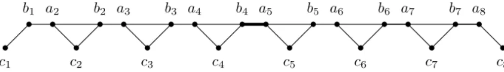
ITheorem 5.5. For every c ∈ N, there is a graph G with bd(G) ≤ c that contains a minimal blocking set of size 2c.
Proof. Recall the notion of triangle-path from Definition 4.9. For t ≥ 2, let a truncated
triangle-path of length t be the graph Ut obtained from a triangle-path of length t by
removing vertices a1 and bt; see Figure 2. Analogously to Observation 4.10, we show
that Yt:= {ci | i ∈ [t]} is a minimal blocking set in Ut. Since Ytis an independent set of
size t, while (the remainders of) the triangles in Utpartition the vertices of Utinto t cliques, it
follows that α(Ut) = t. The set Ytis a blocking set, since Ut\ Ytis a path on 2(t − 1) vertices,
whose independence number is only t − 1. Finally, it is easy to see that for any y ∈ Yt,
there is a size-t independent set in Ut\ (Yt\ y) that consists of the vertex y and, for every
a2 b2 a3 b3 a4 b4 a5 b5 c6 c5 c4 c3 c2 c1 b1 a6 b6 a7 b7 a8 c7 c8
Figure 2 Truncated triangle path U8 of length 8, illustrating Theorem 5.5. Removing the fat
middle bridge and its incident vertices, leaves two connected components isomorphic to U4.
Hence Ut has a minimal blocking set of size t, for all t ≥ 2. To prove the theorem,
it therefore suffices to show that bd(U2c) ≤ c for all c ∈ N. We prove this by induction
on c. For c = 1, note that the graph U2 is just the four-vertex path. Hence it is a forest, implying bd(U2) = 1 by Proposition 3.2. For c > 1, consider the graph U2c. By construction,
the middle edge e = {b2c−1, a2c−1+1} is a bridge in U2c. Let T be the tree in U2c consisting
of the single bridge e. Note that removing V (T ) splits U2c evenly, into two connected
components that are both isomorphic to U2c−1. By induction, bd(U2c−1) ≤ c − 1. Then
Proposition 3.2 shows that bd(U2c) ≤ 1 + bd(Ut\ V (T )) = 1 + (c − 1) = c. J
6
Kernelization for modulators to bounded bridge-depth
To establish the positive direction of Theorem 1.1, we develop a polynomial kernel for Vertex Cover parameterized by the size of a modulator X whose removal leaves a graph of constant bridge-depth; an approximately optimal such set X can be computed using Proposition 3.5. As the kernelization is technical and consists of many different reduction rules, with a nontrivial size analysis, the material is deferred to the full version [4]. In this limited space, we present the high-level idea behind the kernelization and the role of bridge-depth.
Consider an instance (G, k) of Vertex Cover with a modulator X such that bd(G\X) ∈ O(1). As explained in the introduction, using the fact that minimal blocking sets for the components C of G \ X have bounded size, the number of such components can easily be bounded by |X|O(1). To bound the size of individual components, the definition of bridge-depth ensures that in each connected component C of G \ X there is a tree of bridges T ⊆ E(C) (called a lowering tree) such that removing the vertex set V (T ) from C decreases the bridge-depth of C. By designing new problem-specific reduction rules, we shrink the tree of bridges to size polynomial in the parameter. This is where the main technical work of the kernelization step lies. It properly subsumes the earlier kernelization for the parameterization by distance to a forest, which is imported as a black box in all previous works [5, 17–19, 27]. Having bounded the number of components of G \ X, together with the size of a lowering tree of bridges in each component, we now proceed as follows: in each component C of G \ X we move the vertices from a lowering tree of bridges into the set X. This blows up |X| by a polynomial factor, but strictly decreases the bridge-depth of the graph G \ X. We then recursively kernelize the resulting instance. When the bridge-depth of G \ X reaches zero, the graph G \ X is empty and the kernelization is completed. Full details can be found in the full version [4].
The negative direction of Theorem 1.1 is much easier to establish. Using the fact that a minor-closed family F of unbounded bridge-depth contains all triangle paths, a kernelization lower bound for modulators to such F follows easily using known gadgets.
7
Conclusion
In this paper we introduced the graph parameter bridge-depth and used it to characterize the minor-closed graph classes F for which Vertex Cover parameterized by F-modulator has a polynomial kernel. It would be interesting to see whether the characterization can be extended to subgraph-closed or even hereditary graph classes. If a characterization exists of the hereditary graph classes whose modulators lead to a polynomial kernel, it will likely not be as clean as Theorem 1.1: it will have to deal with the fact that bipartite graphs can be arbitrarily complex in terms of width parameters, while bipartite modulators allow for a polynomial kernel. Hence such a characterization has to capture parity conditions of F .
A natural attempt to generalize our approach to deal with bipartite graphs is to consider the following parameter, which we call bipartite-contraction-depth: we mimic the definition of bridge-depth (cf. Definition 3.1), except that we redefine the graph Gcb to be the graph obtained from G by simultaneously contracting all edges that do not lie on an odd cycle. Note that bipartite-contraction-depth generalizes bridge-depth, in the sense that bridges do not lie on an odd cycle, and that the bipartite-contraction-depth of a graph with an odd cycle transversal of size k is at most k + 1. Having defined this parameter, we would need, in order to obtain a statement similar to Theorem 4.14, that large bipartite-contraction-depth implies the existence of structures that allow to obtain kernel lower bounds, similarly to the fact that large bridge-depth implies the existence of large triangle-paths (cf. Corollary 4.13). The appropriate structure here seems to be an odd-cycle-path of length t, defined as a set of t vertex-disjoint odd cycles C1, . . . , Ct, and a set of t − 1 vertex-disjoint paths (of any
length) connecting Ci to Ci+1 for i ∈ [t − 1], in such a way that for every i ∈ {2, . . . , t − 1},
the two attachment vertices in Ci are distinct. Now the expected property would be that
large bipartite-contraction-depth forces long odd-cycle-paths. Unfortunately, this is not true. Indeed, consider the Escher wall of size h depicted in [33, Fig. 3]. It is proved in [33] that this graph does not contain two vertex-disjoint odd cycles, but a smallest hitting set for odd cycles has size h. Since there are no two vertex-disjoint cycles, a longest odd-cycle-path has length one. On the other hand, it can be easily verified that an Escher wall of size h has bipartite-contraction-depth Ω(h). Informally, this can be seen by noting that, initially, all edges lie on an odd cycle, hence a vertex removal is required, and that each such removal cascades in a constant number of contractions until all edges lie again on an odd cycle. Since a smallest hitting set for odd cycles of an Escher wall of size h has size h, the claimed bound follows. Therefore, summarizing this discussion, if one aims at a result similar to Theorem 1.1 that also applies to families F containing bipartite graphs, it seems that significant new ideas are required.
Another open research direction consists of a further algorithmic exploration of the merits of bridge-depth. We expect that several polynomial-space fixed-parameter tractable algorithms that work for graphs of bounded tree-depth [7, 32] can be extended to work with bridge-depth instead. Which other ways to enrich the recursive definition of tree-depth lead to novel algorithmic insights? As for kernelization purposes, it is plausible that bridge-depth also characterizes the existence of polynomial kernels for other problems other than Vertex Cover, parameterized by the vertex-deletion distance of the input graph to a minor-closed graph class.
References
1 Hans L. Bodlaender. A linear-time algorithm for finding tree-decompositions of small treewidth.
SIAM J. Comput., 25(6):1305–1317, 1996. doi:10.1137/S0097539793251219.
2 Hans L. Bodlaender. A partial k-arboretum of graphs with bounded treewidth. Theor. Comput.
Sci., 209(1-2):1–45, 1998. doi:10.1016/S0304-3975(97)00228-4.
3 Hans L. Bodlaender. Kernelization, exponential lower bounds. In Encyclopedia of Algorithms, pages 1013–1017. Springer, 2016. doi:10.1007/978-1-4939-2864-4_521.
4 Marin Bougeret, Bart M. P. Jansen, and Ignasi Sau. Bridge-Depth Characterizes which Struc-tural Parameterizations of Vertex Cover Admit a Polynomial Kernel. CoRR, abs/2004.12865, 2020. arXiv:2004.12865.
5 Marin Bougeret and Ignasi Sau. How much does a treedepth modulator help to obtain polynomial kernels beyond sparse graphs? Algorithmica, 81(10):4043–4068, 2019. doi: 10.1007/s00453-018-0468-8.
6 Jannis Bulian and Anuj Dawar. Graph isomorphism parameterized by elimination distance to bounded degree. Algorithmica, 75(2):363–382, 2016. doi:10.1007/s00453-015-0045-3. 7 Li-Hsuan Chen, Felix Reidl, Peter Rossmanith, and Fernando Sánchez Villaamil. Width, depth,
and space: Tradeoffs between branching and dynamic programming. Algorithms, 11(7):98, 2018. doi:10.3390/a11070098.
8 Marek Cygan, Fedor V. Fomin, Lukasz Kowalik, Daniel Lokshtanov, Dániel Marx, Marcin Pilipczuk, Michal Pilipczuk, and Saket Saurabh. Parameterized Algorithms. Springer, 2015. doi:10.1007/978-3-319-21275-3.
9 Marek Cygan, Daniel Lokshtanov, Marcin Pilipczuk, Michal Pilipczuk, and Saket Saurabh. On the hardness of losing width. Theory Comput. Syst., 54(1):73–82, 2014. doi:10.1007/ s00224-013-9480-1.
10 Holger Dell and Dieter van Melkebeek. Satisfiability allows no nontrivial sparsification unless the polynomial-time hierarchy collapses. J. ACM, 61(4):23:1–23:27, 2014. doi:10.1145/2629620. 11 Reinhard Diestel. Graph Theory. Springer-Verlag, Heidelberg, 5th edition, 2016.
12 Rod G. Downey and Michael R. Fellows. Fundamentals of Parameterized Complexity. Texts in Computer Science. Springer, 2013.
13 Michael R. Fellows, Lars Jaffke, Aliz Izabella Király, Frances A. Rosamond, and Mathias Weller. What is known about vertex cover kernelization? In Hans-Joachim Böckenhauer, Dennis Komm, and Walter Unger, editors, Adventures Between Lower Bounds and Higher
Altitudes - Essays Dedicated to Juraj Hromkovič on the Occasion of His 60th Birthday,
volume 11011 of Lecture Notes in Computer Science, pages 330–356. Springer, 2018. doi: 10.1007/978-3-319-98355-4_19.
14 Jörg Flum and Martin Grohe. Parameterized Complexity Theory. Springer-Verlag, 2006. doi:10.1007/3-540-29953-X.
15 Fedor V. Fomin, Daniel Lokshtanov, Neeldhara Misra, Geevarghese Philip, and Saket Saurabh. Hitting forbidden minors: Approximation and kernelization. SIAM J. Discrete Math., 30(1):383– 410, 2016. doi:10.1137/140997889.
16 Fedor V. Fomin, Daniel Lokshtanov, Saket Saurabh, and Meirav Zehavi. Kernelization:
Theory of Parameterized Preprocessing. Cambridge University Press, 2019. doi:10.1017/
9781107415157.
17 Fedor V. Fomin and Torstein J. F. Strømme. Vertex cover structural parameterization revisited. In Proc. 42nd WG, volume 9941 of LNCS, pages 171–182, 2016. doi:10.1007/ 978-3-662-53536-3_15.
18 Eva-Maria C. Hols and Stefan Kratsch. Smaller parameters for vertex cover kernelization. In
Proc. 12th IPEC, volume 89 of LIPIcs, pages 20:1–20:12, 2017. doi:10.4230/LIPIcs.IPEC.
2017.20.
19 Eva-Maria C. Hols, Stefan Kratsch, and Astrid Pieterse. Elimination distances, blocking sets, and kernels for vertex cover. In Proc. 37nd STACS, volume 154 of LIPIcs, pages 36:1–36:14, 2020. doi:10.4230/LIPIcs.STACS.2020.36.