HAL Id: tel-01101218
https://hal.inria.fr/tel-01101218
Submitted on 8 Jan 2015HAL is a multi-disciplinary open access
archive for the deposit and dissemination of sci-entific research documents, whether they are
pub-L’archive ouverte pluridisciplinaire HAL, est destinée au dépôt et à la diffusion de documents scientifiques de niveau recherche, publiés ou non,
retinal pathways in the early thalamocortical visual
system
Carlos Carvajal
To cite this version:
Carlos Carvajal. Dynamic interplay between standard and non-standard retinal pathways in the early thalamocortical visual system: A modeling study. Neuroscience. Université de Lorraine, 2014. English. �tel-01101218�
Dynamic interplay between standard
and non-standard retinal pathways in
the early thalamocortical visual system:
A modeling study
THESIS
submitted and defended publicly on December the 17th, 2014 in partial fulfillment of the requirements for the degree of
Doctor of Science
Specialized in Computer Scienceby
Carlos Carvajal
Thesis CommitteeAdvisor Dr. Fr´ed´eric Alexandre Inria Bordeaux Sud-Ouest
Co-advisor Dr. Thierry Vi´eville Inria Sophia Antipolis M´editerran´ee Reviewers Dr. Lionel Nowak CNRS
Dr. H´el`ene Paugam-Moisy Universit´e Lyon 2
Examiners Dr. Benoˆıt Miramond Universit´e Cergy-Pontoise Dr. Sylvain Contassot-Vivier Universit´e de Lorraine Dr. Adri´an Palacios Universidad de Valpara´ıso
Interaction dynamique entre les voies
r´
etiniennes standard et non-standard
dans le syst`
eme visuel thalamocortical
pr´
ecoce : Une ´
etude de mod´
elisation
TH`
ESE
pr´esent´ee et soutenue publiquement le 17 D´ecembre 2014 pour l’obtention du
Doctorat en Sciences
Sp´ecialit´e Informatique parCarlos Carvajal
Comit´e de th`eseDirecteur Dr. Fr´ed´eric Alexandre Inria Bordeaux Sud-Ouest
Co-directeur Dr. Thierry Vi´eville Inria Sophia Antipolis M´editerran´ee Rapporteurs Dr. Lionel Nowak CNRS
Dr. H´el`ene Paugam-Moisy Universit´e Lyon 2
Examinateurs Dr. Benoˆıt Miramond Universit´e Cergy-Pontoise Dr. Sylvain Contassot-Vivier Universit´e de Lorraine Dr. Adri´an Palacios Universidad de Valpara´ıso
I would like to thank everybody with whom I have shared this PhD experience. Too many names to write them all, but you are all in my heart one way or another.
I would like to start the personal thanks with my advisors, M. Fr´ed´eric Alexandre and M. Thierry Vi´eville, for allowing me to live this PhD experience the way it went professionally, for their guidance, advises, discussions and all the nice moments we shared along the way.
I would also like to thank M. Nicolas Rougier, who at quite a few times was there to share a precise advise, and the people from KEOpS, specially Mme. Mar´ıa-Jos´e Es-cobar, and M. Adri´an Palacions, without whom I would have never started working in computational neuroscience, or research.
I thank the reviewers of this manuscript, Mme. H´el`ene Paugam-Moisy and M. Lionel Nowak, as well as the examiners, M. Benoˆıt Miramond, M. Sylvain Contassot-Vivier and M. Adri´an Palacios, for accepting to review my work, and for their constructive feedback. I cannot forget to thank all the people at Loria, Inria Nancy, IMN and Inria Bordeaux, specially the team assistants of Cortex and Mnemosyne, who had more than one headache dealing with my paperwork... Mme. Laurence Benini, Mme. Anne-Laure Gauthier, M. Nicolas Jahier, and Mme. Chrystel Plumejeau.
I met so many people and lived so many things during these three years... I thank my officemates in Nancy, specially Georgios; the people that allowed me to participate in so many scientific outreach activities when in Bordeaux, particularly Mlle. Lola Kovacic; the people who trusted me with special responsibilities, despite being my initiative to be there, particularly the people in the committee of the center, SO News, and the AFoDIB; the people from the different sportive activities funded by AGOS (and AGOS too): foot-ball, foosball and climbing; and all the beautiful people at the Inria Bordeaux Sud-Ouest Research Center for always being so nice to me.
I cannot allow myself not to mention my close friends... Flo, Fred, Arnaud and Anca, Polina, and Marinette. Thanks for being there for me, for trusting me, for sharing trips, musical evenings, secrets, moments of joy and sadness, and the beauty of life in general.
I also thank my family. My mother, Isabel; my father, Carlos; and my “little” brother, Camilo. Despite a great geographical distance separating us at the moment, I know you are there for me.
Understanding the behavior of the retino-thalamo-cortico-collicular (i.e. early) visual system in a natural images situation is of utmost importance to understand what further happens in the brain. To understand these behaviors, neuroscientists have looked at the standard Parvocellular and Magnocellular pathways for decades. However, there is also the non-standard Koniocellular pathway, which plays an important modulating role in the local, global, and intermingled processing carried out to achieve such behaviors. Particularly, the standard motion analysis carried out by the Magno pathway is alternated with rapid reactions, like fleeing or approaching to specific motions, which are hard-wired in the Konio pathway. In addition, studying a fixation task in a real situation, e.g., when a predator slowly approaches its prey, not only involves a motion mechanism, but also requires the use of the Parvo pathway, analyzing, at least, the image contrast. Here, we study in a bio-inspired computational neural model how these pathways can be modeled with a minimal set of parameters, in order to provide robust numerical results when doing a real task. This model is based upon an important study to integrate biological elements about the architecture of the circuits, the time constants and the operating characteristics of the different neurons. Our results show that our model, despite operating via local computations, globally shows a good network behavior in terms of space and time, and allows to analyze and propose interpretations to the interplay between thalamus and cortex. At a more macroscopic scale, the behaviors emerging from the model are reproducible and can be qualitatively compared to human-made fixation measurements. This is also true when using natural images, where just a few parameters are slightly modified, keeping the qualitatively human-like results. Robustness results show that the precise values of the parameters are not critical, but their order of magnitude matters. Numerical instability occurs only after a 100% variation of a parameter. We thus can conclude that such a reduced systemic approach is able to represent attentional shifts using natural images, while also being algorithmically robust. This study gives us as well a possible interpretation about the role of the Konio pathway, while at the same time allowing us to participate in the debate between low and high-roads in the attentional and emotional streams. Nevertheless, other information, such as color, is also present in the early visual system, and should be addressed together with more complex cortical mechanisms in a sequel of this work.
Keywords: Early visual system, Behavior, Neural modeling, Thalamocortical pathways, Computational Neuroscience, Visual attention.
Comprendre le comportement du syst`eme visuel r´etino-thalamo-cortico-colliculaire (i.e. pr´ecoce) dans une situation d’images naturelles est d’une importance capitale pour comprendre ce qui se passe ensuite dans le cerveau. Pour comprendre ces comportements, les neurobiologistes ont ´etudi´e les voies standard, Parvocellulaires et Magnocellulaires, depuis des d´ecennies. Cependant, il y a aussi la voie non-standard, ou Koniocellulaire, qui joue un rˆole modulateur important dans les traitements local, global, et entremˆel´e, pour atteindre de tels comportements. Particuli`erement, l’analyse standard du mouvement r´ealis´ee par la voie Magno est altern´ee avec des r´eactions rapides, comme la fuite ou l’approche `a des mouvements sp´ecifiques, qui sont pr´e-cˆabl´es dans la voie Konio. De plus, l’´etude d’une tˆache de fixation dans une situation r´eelle, par exemple quand un pr´edateur s’approche lentement de sa proie, implique non seulement un m´ecanisme de mouvement, mais n´ecessite ´egalement l’utilisation de la voie Parvo, qui analyse, au moins, le contraste de l’image. Ici, nous ´etudions dans un mod`ele neuronal de calcul bio-inspir´e comment ces voies peuvent ˆetre mod´elis´ees avec un ensemble minimal de param`etres, afin de fournir des r´esultats num´eriques robustes lors d’une tˆache r´eelle. Ce mod`ele repose sur une ´etude approfondie pour int´egrer des ´el´ements biologiques dans l’architecture des circuits, les constantes de temps et les caract´eristiques de fonctionnement des neurones. Nos r´esultats montrent que notre mod`ele, bien que fonctionnant via des calculs locaux, montre globalement un bon comportement de r´eseau en termes d’espace et de temps, et permet d’analyser et de proposer des interpr´etations de l’interaction entre le thalamus et le cortex.
`
A une ´echelle plus macroscopique, les comportements du mod`ele sont reproductibles et peuvent ˆetre qualitativement compar´es `a des mesures de fixation oculaire chez l’homme. Cela est ´egalement vrai lorsque l’on utilise des images naturelles, o`u quelques param`etres sont l´eg`erement modifi´es, en gardant des r´esultats qualitativement humains. Les r´esultats de robustesse montrent que les valeurs pr´ecises des param`etres ne sont pas critiques, mais leur ordre de grandeur l’est. Une instabilit´e num´erique ne se produit qu’apr`es une variation de 100% d’un param`etre. Nous pouvons donc conclure que cette approche syst´emique est capable de repr´esenter les changements de l’attention en utilisant des images naturelles, tout en ´etant algorithmiquement robuste. Cette ´etude nous donne ainsi une interpr´etation possible sur le rˆole de la voie Konio, tandis qu’en mˆeme temps elle nous permet de participer au d´ebat sur les low et high-roads des flux attentionnel et ´emotionnel. N´eanmoins, d’autres informations, comme la couleur, sont ´egalement pr´esentes dans le syst`eme visuel pr´ecoce, et pourraient ˆetre prises en consid´eration, ainsi que des m´ecanismes corticaux plus complexes, dans les perspectives de ce travail.
Mots cl´es : Syst`eme visuel pr´ecoce, Comportement, Mod´elisation neuronale, Voies thalamocorticales, Neuroscience computationnelle, Attention visuelle.
BG Basal Ganglia
DANA Distributed Asynchronous Numerical and Adaptive computing framework DoG Difference of Gaussians
DNF Dynamic Neural Field dSC Deep Superior Colliculus FEF Frontal Eye Field
GC Ganglion Cell IF Integrate and Fire IT Inferior Temporal Cortex LGN Lateral Geniculate Nucleus LIP Lateral Intraparietal Cortex MST Medial Superior Temporal Area Pdm Dorsomedial Pulvinar
PI Inferior Pulvinar PL Lateral Pulvinar RF Receptive Field SC Superior Colliculus
sSC Superficial Superior Colliculus SVM Support Vector Machine TRN Thalamic Reticular Nucleus V1 Primary Visual Cortex
Acknowledgements i
Abstract iii
R´esum´e v
Symbols vii
Contents ix
List of Figures xiv
List of Tables xvi
Introduction xviii
Introduction (Fran¸cais) xxi
1 Neuroscience of the early visual system of primates 1 1.1 Introduction: Overview of the early visual system . . . 3 1.2 The retina: The smart front-end . . . 5
1.2.4 Projections of ganglion cells: The birth of visual pathways . . . 13
1.3 The cortex: The adaptable mainframe . . . 15
1.4 The thalamus: The collaborative harmonizer . . . 20
1.4.1 Properties of thalamic structures . . . 24
1.4.2 The complex relay: the lateral geniculate nucleus . . . 26
1.4.3 Konio pathway and its projections . . . 27
1.4.4 The inhibition center: the thalamic reticular nucleus . . . 29
1.4.5 The higher-order thalamic nucleus: briefing of the pulvinar . . . 29
1.5 The superior colliculus: The early sensory-motor hookup . . . 30
1.6 The amygdala: The mnesic and emotional muscle . . . 31
1.6.1 A few facts about the amygdala . . . 31
1.6.2 Amygdala and perception: attention and (un)awareness . . . 31
1.7 Temporal aspects of the early visual system . . . 33
1.8 Summary: A circuit of loops and interacting flows . . . 34
2 Bio-inspired dynamical systems and algorithms 38 2.1 Implementing populations of neurons: the notion of minimal model . . . 41
2.1.1 Spike vs rate models: why we have made the standard choice . . . . 41
2.1.2 Driver/Modulator considerations . . . 46
2.1.3 Specification and validation of parameter values . . . 50
2.1.4 Filters and information processing . . . 51
2.1.5 Dynamic Neural Fields . . . 53
2.2 Functional view of the neural system: the systemic level . . . 54
2.2.1 Functional interpretation of retinal mechanisms: non-local filtering . 54 2.2.2 Functional interpretation of retinal mechanisms: visual event detection 56 2.2.3 Functional interpretation of thalamic mechanisms . . . 59
2.2.4 Assembling populations into networks . . . 60
2.2.5 Implementation details . . . 62
3.1.1 Architecture of the system . . . 69
3.1.2 Dynamics of the system . . . 70
3.2 Our model of the early visual system: modular view . . . 71
3.2.1 Retina: Standard and non-standard cells . . . 73
3.2.2 Thalamus . . . 75
3.2.3 Primary visual cortex . . . 79
3.2.4 Superior colliculus . . . 79
3.2.5 Summary . . . 82
4 Our minimal model in the real world: Experimental results 84 4.1 First experimental result: using artificial images . . . 87
4.1.1 Discrimination, selection and tracking . . . 89
4.1.2 Numerical Robustness . . . 89
4.2 Original experimental result: using natural images (M+K) . . . 95
4.2.1 Discrimination, selection and tracking . . . 97
4.2.2 Numerical robustness . . . 102
4.3 Experimental result: using natural images (P+M+K) . . . 104
4.4 About observed emerging properties . . . 116
4.5 Open-access software . . . 116
5 Conclusion 118
6 Conclusion (Fran¸cais) 123
Appendix 128
1.1 Gross architecture of the early visual system . . . 4
1.2 Diversity of neurons in the retina . . . 6
1.3 The road in the retina . . . 7
1.4 Circuitry in the retina . . . 8
1.5 Receptive fields with irregular shapes . . . 10
1.6 Dendritic morphology of macaque ganglion cells . . . 12
1.7 Different retinal projections . . . 14
1.8 Simplified cortical column . . . 16
1.9 Integration of information through thalamocortical and corticocortical in-teractions . . . 21
1.10 Overview of thalamic nuclei . . . 22
1.11 Thalamocortical connections and how TRN is involved . . . 23
1.12 Schematic diagram of circuitry for the lateral geniculate nucleus . . . 28
1.13 Cortical and subcortical visual and emotional pathways . . . 32
3.1 Model diagram . . . 72
4.1 Sample of artificial stimuli used . . . 88
4.2 Simulation results for “d” . . . 90
4.3 Simulation results for “Se” . . . 91
4.4 Simulation results for “d” with variations of a9 . . . 92
4.5 Simulation results for “d” with variations of g9 . . . 93
4.6 Simulation results for “d” with variations of K . . . 94
4.7 Simulation results for “d” with variations of τ11 . . . 95
4.12 TRN and mismatch in action . . . 101
4.13 Simulation results for all three systems with natural images . . . 103
4.14 Variation of the simulation results for g9 . . . 105
4.15 Variation of the simulation results for Z . . . 106
4.16 Variation of the simulation results for K . . . 107
4.17 Overview of results with natural stimuli in the P+M+K system . . . 109
4.18 Parasol cells detect motion . . . 110
4.19 Appearance of the fearful stimulus . . . 110
4.20 Focus switch occurs . . . 111
4.21 Parvo and Magno convergence . . . 111
4.22 Parasol cells detect motion, but do not transmit it to LGN . . . 113
4.23 Appearance of the fearful stimulus . . . 113
4.24 Focus switch occurs cortically, but it is not yet reflected collicularly . . . 114
4.25 Convergence of the lesioned system . . . 114
4.26 Simulation results for the P+M+K systems . . . 115
6.1 Overview of simulation using Eli P-jump . . . 130
6.2 Overview of simulation using the video of a puppy dog . . . 131
1.1 Anatomical circuitry and functions of V1 connections . . . 17 1.2 Summary of anatomical circuitry of early thalamocortical loops of mammals 19 1.3 Neural dynamics in the visual system . . . 35 2.1 Forward/Backward connections connections main properties, from [54].
Post-synaptic/modulatory effect is a conjecture, so is assumptions on synapses mechanisms. . . 48 2.2 Notations used in the different equations . . . 65 3.1 Handpicked values for the computations on Core Thalamus . . . 76 3.2 Handpicked values for the computations on TRN . . . 78 3.3 Handpicked values for the computations on the integrative cortex . . . 80 3.4 Handpicked values for the computations on layer 2a of the superior colliculus 80 3.5 Handpicked values for the computations on layer 2b of the superior colliculus 81 3.6 Handpicked values for the computations on the deep superior colliculus . . 82 4.2 Variations from Magno to Parvo values . . . 108 4.1 Numerical Robustness for parameters used with natural stimuli . . . 117
“The beginning is the most important part of the work” – Plato
Understanding how the brain works is arguably one of the greatest scientific challenges nowadays. There are two particularly massive initiatives trying to approach the challenge: one is the Human Brain Project1, in Europe; and the other is the BRAIN Initiative, in
the US2. However, this huge challenge is also attacked by many research labs, beyond such very mediatic consortium, as our team.
Among the processing carried out by the brain, more than a quarter of it is dedicated to vision [174]. And despite decades of research, the mystery of vision [107] remains partially unsolved. One possibility is that the difficulty to understand what happens in the brain is a result of our lack of understanding of the earlier visual stages. This includes what the brain receives, and how it is encoded, but also why (in terms of functionality) such information has been developed along evolution.
The key point is that, through several studies, researchers have assumed that the retina (in the eye) was practically a simple transducer, while the thalamus (between the eye and the cortex) served as a simple relay of information towards the neocortex. Thus, under these assumptions, almost every task should be accomplished by the cortex, from a processing point of view. However, as scientists have explored these areas, they have found that there is much, much more than previously thought. For example, sophisticated processing such as detection of complex patterns (including motion and color) is already found in the retina. In a coarse way, it provides enough information to guide actions [62]. This (e.g. rapid detection of snakes in the pulvinar [176]), together with multi-modal synchronization
1
olution than that provided by the state of the art equipment. We thus can observe in vivo behavior of one neuron or a sub-population of neurons, in detail, thanks to electrode arrays, or mesoscopic or macroscopic aspects of the brain activity at rather higher spatial scale but low temporal precision (e.g., fMRI or optical imaging) or low spatial scale and high temporal resolution (e.g., E.E.G. or M.E.G.). Fortunately, when looking at it from a functional, global perspective, today we can already infer new things that can be tested at more detailed levels, using numerical experiments. With methods related to those used by engineers to design new airplanes, we are now able to simulate some aspects of the central nervous system behavior, and derive some new findings from such experimentation.
This key point is our motivation to investigate further how the early visual system works, how the neurons code information at the scale of neural maps and raise assumptions about how the brain may process such information. We will carefully explain how minimal models are to be worked out in such a paradigm. This does not negate the huge processing power of the different cortical areas. We simply support the trend of showing that certain aspects of this processing are to be made explicit and studied. We also consider that the visual system is really a distributed processing system as far as analyzing the information captured from the visual world is concerned.
This work has been realized under the Franco-Chilean project KEOpS. The goal of the project is to study and model the early visual system, focusing on the non-standard behavior of retinal ganglion cells in natural scenarios. The retina is the first stage in the visual system, and understanding it better is expected to provide more knowledge to understand the following stages of the visual system, and eventually the brain, since they rely not only on “image input”, but also on the processing carried out in the visual front-end to the different information flows.
This thesis also contributes to one application of KEOpS, i.e., to incorporate the re-sulting models into real engineering applications as new dynamic early-visual modules able to process natural image sequences.
Here, standard and non-standard retinal flows are combined, from the retina to the primary visual cortex, including thalamic and collicular structures. The idea is to close the early visual system loop, with a special focus on attentional mechanism. This beautiful mess is analyzed, modeled locally, but always having the systemic view in mind: complex
increased in complexity or amount only if really needed. This approach allows us to pro-vide a relatively straightforward tool to analyze the early visual system, where the results qualitatively reproduce human behavior while using sequences of natural images, and at the same time provides robust, stable and easily modifiable modules for each structure involved.
“Le d´ebut est la partie la plus importante du travail” – Platon
Comprendre comment fonctionne le cerveau est sans doute l’un des plus grands d´efis scientifiques de nos jours. Il y a deux initiatives particuli`erement massives qui tentent d’aborder le d´efi : l’un est le Human Brain Project3, en Europe; et l’autre est l’initiative
BRAIN, aux ´Etats-Unis4. Toutefois, ce d´efi est aussi attaqu´e par de nombreux laboratoires de recherche, au-del`a de ce consortium tr`es m´ediatique, comme notre ´equipe.
Parmi les traitements effectu´es par le cerveau, plus d’un quart d’entre eux est d´edi´e `a la vision [174]. Et malgr´e des d´ecennies de recherche, le myst`ere de la vision [107] ne reste que partiellement r´esolu. Une possibilit´e est que la difficult´e `a comprendre ce qui se passe dans le cerveau soit le r´esultat de notre manque de compr´ehension des ´etapes visuelles pr´ecoces. Cela comprend ce que le cerveau re¸coit, et comment cette information est cod´ee, mais aussi pourquoi (en termes de fonctionnalit´e) de telles informations ont ´et´e d´evelopp´ees au cours de l’´evolution.
Le point cl´e est que, `a travers plusieurs ´etudes, les chercheurs ont consid´er´e la r´etine (dans l’oeil) pratiquement comme un transducteur simple, tandis que le thalamus (entre l’oeil et le cortex) comme un simple relais de l’information vers le n´eocortex. Ainsi, sous ces hypoth`eses, presque chaque tˆache doit ˆetre accomplie par le cortex, du point de vue du traitement. Cependant, plus les scientifiques ont explor´e ces zones, plus ils ont trouv´e qu’il y avait beaucoup, beaucoup plus qu’on ne le pensait. Par exemple, des traitements sophis-tiqu´es tels que la d´etection de motifs complexes (y compris le mouvement et la couleur) sont d´ej`a pr´esents dans la r´etine. D’une mani`ere grossi`ere, la r´etine fournit suffisamment
3
et la d´etection rapide des serpents dans le pulvinar [176].
Nous avons aussi la question pratique de la technologie : nous ne pouvons pas mesurer avec une r´esolution sup´erieure `a celle pr´evue par l’´equipement de pointe. Nous pouvons ainsi observer le comportement in vivo d’un neurone ou d’une sous-population de neurones, en d´etail, grˆace aux matrices d’´electrodes, ou des aspects m´esoscopiques ou macroscopiques de l’activit´e c´er´ebrale `a des ´echelles spatiales plus ´elev´ees, mais avec une faible pr´ecision temporelle (par exemple, avec les IRMf ou l’imagerie optique) ou une faible ´echelle spa-tiale et une haute r´esolution temporelle (par exemple, avec EEG ou MEG). Heureuse-ment, quand on regarde les choses d’un point de vue global, fonctionnel, aujourd’hui, nous pouvons d´ej`a d´eduire de nouvelles choses qui peuvent ˆetre test´ees `a des niveaux plus d´etaill´es, par des exp´eriences num´eriques. Avec des m´ethodes li´ees `a celles utilis´ees par les ing´enieurs pour concevoir de nouveaux avions, nous sommes maintenant en mesure de simuler certains aspects du comportement du syst`eme nerveux central, et de d´eriver, de ces exp´erimentations, de nouvelles conclusions.
Ce point cl´e est notre motivation pour ´etudier plus loin comment fonctionne le syst`eme visuel pr´ecoce, comment les neurones codent les informations `a l’´echelle des cartes neu-rales, et pour proposer des hypoth`eses sur la fa¸con dont le cerveau peut traiter de telles informations. Nous allons expliquer soigneusement comment les mod`eles minimaux doivent ˆetre travaill´es dans un tel paradigme. Cela ne remet pas en cause l’´enorme puissance de traitement des diff´erentes aires corticales. Nous tentons simplement de montrer que cer-tains aspects de ce traitement doivent ˆetre rendus explicites et ´etudi´es. Nous consid´erons ´egalement que le syst`eme visuel est vraiment un syst`eme de traitement distribu´e d`es que l’analyse de l’information recueillie `a partir du monde visuel est concern´e.
Ce travail a ´et´e r´ealis´e dans le cadre du projet Franco-Chilien KEOpS. Le but du projet est d’´etudier et de mod´eliser le syst`eme visuel pr´ecoce, mettant l’accent sur le comportement non-standard des cellules ganglionnaires de la r´etine dans des sc´enarios naturels. La r´etine est la premi`ere ´etape dans le syst`eme visuel, et mieux la comprendre devrait fournir plus de connaissances pour comprendre les ´etapes suivantes du syst`eme visuel, et, ´eventuellement, du cerveau, car ces ´etapes reposent non seulement sur l’image d’entr´ee, mais ´egalement sur le traitement effectu´e sur les diff´erentes flux d’information
veaux modules dynamiques de vision pr´ecoce, capables de traiter des s´equences d’images naturelles.
Ici, les flux r´etiniens standard et non-standard sont combin´es, de la r´etine au cor-tex visuel primaire, y compris des structures thalamiques et colliculaires. L’id´ee est de fermer la boucle du syst`eme visuel pr´ecoce, avec un accent particulier sur le m´ecanisme d’attention. Ce syst`eme est analys´ee et mod´elis´ee localement, mais en gardant toujours la vue syst´emique `a l’esprit : les propri´et´es complexes ne doivent pas ˆetre cˆabl´ees dans le syst`eme, mais doivent `a la place ´emerger des diff´erentes interactions entre les structures et les connexions.
Puisque nous d´eveloppons des mod`eles minimaux, mais sans perte de g´en´eralit´e, la quantit´e de param`etres, et les m´ecanismes utilis´es pour repr´esenter les circuits du monde r´eel, sont simplifi´es et augment´es en complexit´e ou en montant seulement si c’est vraiment n´ecessaire. Cette approche nous permet de fournir un outil relativement simple –peu de param`etres et tr`es facile `a adapter– pour analyser le syst`eme visuel pr´ecoce, o`u les r´esultats reproduisent qualitativement le comportement humain lors de l’utilisation de s´equences d’images naturelles, et en mˆeme temps fournit des modules robustes, stables et facilement modifiables pour chaque structure impliqu´ee.
Neuroscience of the early visual
system of primates
Contents
1.1 Introduction: Overview of the early visual system . . . 3 1.2 The retina: The smart front-end . . . 5 1.2.1 The notion of receptive field . . . 9 1.2.2 Standard ganglion cells . . . 11 1.2.3 Non-standard ganglion cells . . . 11 1.2.4 Projections of ganglion cells: The birth of visual pathways . . . 13 1.3 The cortex: The adaptable mainframe . . . 15 1.4 The thalamus: The collaborative harmonizer . . . 20 1.4.1 Properties of thalamic structures . . . 24 1.4.2 The complex relay: the lateral geniculate nucleus . . . 26 1.4.3 Konio pathway and its projections . . . 27 1.4.4 The inhibition center: the thalamic reticular nucleus . . . 29 1.4.5 The higher-order thalamic nucleus: briefing of the pulvinar . . . . 29 1.5 The superior colliculus: The early sensory-motor hookup . . . 30 1.6 The amygdala: The mnesic and emotional muscle . . . 31 1.6.1 A few facts about the amygdala . . . 31 1.6.2 Amygdala and perception: attention and (un)awareness . . . 31 1.7 Temporal aspects of the early visual system . . . 33
Summary
New findings regarding the study of the retina and thalamus, due to increasingly more interest to these structures, have led scientists to review their viewpoint in terms of the functionality of these subcortical structures. One keypoint is that processing usually at-tributed to the cortex has been in fact also made explicit -in a new but fast form- in these early vision structures. The retina, on the one hand, providing the visual input for the rest of the system, was considered mainly a transductor. However, some processing, such as looming motion detection, has been found to be part of the mechanisms this two-layer structure carries out as a visual front-end. The thalamus, on the other hand, was classically regarded as a simple relay of feedforward information, but there is much more to add to the story. For example, the thalamus receives neither only visual information, nor solely feed-forward information from early visual regions, but also information from other modalities (e.g. audition), and feedback information from many cortical areas. In addition, the thala-mus boasts inhibitory mechanisms, allowing to regulate, and thus harmonize multi-modal information based on several sources, making it a quite collaborative ensemble.
The goal of this chapter is to gather and present information about the early visual system to establish a ground-base knowledge for further reading of this document, while at the same time teasing the reader on the importance and interest that started this work.
Keywords: Early visual system, Visual pathway, Thalamocortical loops, Neuroscience.
Organization of this chapter:
After a brief introduction of the early visual system, with basic definitions and ideas, its different components are reviewed: the retina, the cortex, the thalamus and the superior colliculus. In addition, we very briefly discuss the amygdala, as understanding further visual processing is crucial for the systemic approach we used to conceive the original work here presented. The chapter is then finished by refreshing and reinforcing the idea that the beautiful mess we here study is a circuit of various loops, where different interacting information flows are the actors, and that these actors work at different time scales, but despite all this, it allows us to marvel at the beauty of the visual world.
1.1
The brain is an amazingly resourceful and complex entity. Arguably, the most demand-ing sense –in terms of processdemand-ing in the cortex of primates– is vision. However, vision starts way before the cortex, in what is called the early visual system.
The early visual system has been previously studied sequentially towards the cortex, but nowadays we know that a series of loops and interacting information flows exist prior to the processing carried out by the cortex.
The early visual system, in simple words, is the ensemble formed by the retina (in the eye), the lateral geniculate nucleus and the thalamic reticular nucleus (in the thalamus), the superficial and deep superior colliculus (in the midbrain), and the primary visual cor-tex. In addition, as if having quite a few structures was not enough, we should consider that all these different structures hold different types of neurons, with different process-ing capabilities and timprocess-ing... Here the conclusion is that there is a quite complex system before the cortex, a beautiful mess, called the early visual system, and that in order to understand what information is fed to the brain, one must embark on the adventure and sail the complex ocean of studying it. Here, many scientists have observed what are now called the “standard” information flows, but there is much more to discover when hoisting the sails to explore the “non-standard” information flows.
In order to provide a deeper understanding of how the early visual system works the way it does, other regions, such as other cortical areas, the pulvinar and the amygdala, are also going to be briefly reviewed in this chapter.
The circuitry/architecture of the early visual system is presented in Figure 1.1. Light penetrates our eyes and is transduced by the retina into a train of spikes after being further processed within the retina. These electric signals are then rearranged at the optic chiasm1 and sent towards further structures. These neuronal structures are mainly the lateral geniculate nucleus (LGN), in the thalamus; and the superior colliculus, in the midbrain. Through LGN, information gets to the primary visual cortex, involving thalamo-cortical loops. Feedforward information is sent to the cortex, and feedback information is sent back to the thalamus by cortical areas. These loops are regulated by a structure called the thalamic reticular nucleus (TRN), which is not present in Figure 1.1. Through the superior colliculus, information arrives to the pulvinar (another structure in the thalamus)
and then to the amygdala. The pulvinar also receives and sends information to and from cortical areas, in thalamocortical loops similar to those of LGN, also regulated by TRN.
Figure 1.1: Gross architecture of the early visual system. Image taken from [69], itself adapted, with permission from [59].
All these are the primary structures to what is called “vision for behavior”, which con-sists not only in regular visual processing for “perceiving”, but also provides the capabilities to act with the environment in close relation to our body, our needs, and our emotions. Or simply said, to properly behave.
themselves receive information from midget and parasol ganglion cells in the retina. The non-standard Konio pathway has been explored more recently, and acts as a modulating stream along the whole early visual system and beyond, thanks to widespread connections to various cortical areas.
Let us describe these structures in more detail.
1.2
The retina: The smart front-end
The retina [45] is the first non-optical stage of the mammalian visual system. It is non-optical in the sense that it is different from the cornea and other parts of the eye, because it transduces light, i.e., converts it into electrical signals.
The mammalian retina is a small tissue located in the back of the eye (Figure 1.3), and is described as a two layered circuit composed by over 50 anatomically different types of cells [105][106](Figure 1.2). These cells are grouped in five categories: the photoreceptors, the bipolar cells, the horizontal cells, the amacrine cells, and the ganglion cells. A connection between neurons is called a synapse, and the connectivity between these different neurons can be seen in Figure 1.4, where colored dots represent excitatory (black) or inhibitory (white) chemical synapses, while electrical synapses (gap-junctions) are represented by those spring-looking symbols, which depict resistors.
Before going deeper in understanding these neurons, one must be reminded a few con-cepts. We call the retina a two-layered structure (cf. Figure 1.4) for all what happens 1) from photoreceptors to bipolar cells, and 2) from bipolar to ganglion cells. There is a special place in the retina called the fovea, which covers about 3 degrees, and contains the neurons that give us the most detailed view we can have of the visual field (the human vi-sual field is approximately 160 degrees horizontally and 135 degrees vertically). One should as well consider that humans have a blind spot, which is basically the retinal surface where the retinal “output-wire”, called the optic nerve, is created, gathering the information of our ganglion cells. We do not notice this blind spot, nor the lesser-quality details outside the fovea, because our eyes move really fast all the time, and also because our brain is able to reconstruct the scene from all these samples, filling gaps when necessary, interpolating, replacing information to make sense of the visual world. And now, let us analyze in more depth the different retinal neurons.
Figure 1.2: Diversity of neurons in the retina. From top to bottom: photoreceptors, horizontal cells, bipolar cells, amacrin cells and ganglion cells. For all these classes, certain types can be identified depending on their morphology and dendritic organization. Image taken from [106].
Figure 1.3: The road in the retina. Light enters the eye through the cornea –the trans-parent cover of our eyes–, to then pass through a chamber full of fluid (called the aqueous humour), in order to reach the iris, which regulates the amount of light that passes through the pupil, the black “spot” on our eyes. Then, the light rays passing through the pupil reach the lens, which turns them upside down and, through another liquid chamber, called the vitreous humour, focuses them into the retina, which is the thin bowl-shaped tissue in the back of the eyeball. Image taken from [56], itself modified from the National Eye Institute, National Institutes of Health.
Figure 1.4: Circuitry in the retina, where P = photoreceptors, H = horizontal cells, B = bipolar cells, A = amacrine cells, and G = ganglion cells. The neurons in the retina are connected through chemical synapses that are either sign preserving (excitatory, closed circles) or sign inverting (inhibitory, open circles). In addition, one finds a considerable amount of electrical coupling between cells via gap junctions within all cell classes and across some types of cells (marked by resistor symbols). The input into the network is inci-dent light, which hyperpolarizes the photoreceptors. The connections from photoreceptors to bipolar cells are of either sign, producing both OFF-type and ON-type bipolars. Hori-zontal cells provide negative feedback and lateral inhibition to photoreceptors and bipolar cells. Bipolar cells are reciprocally connected to amacrine cells with chemical synapses and, for some types, through electrical gap junctions. Ganglion cells represent the output layer of the retina; their axons form the optic nerve. They collect excitation from bipolar cells and mostly inhibition from amacrine cells. In addition, ganglion cells and amacrine cells can be electrically coupled. This general connectivity sets the framework for any specific retinal microcircuit. Image and caption taken from [62].
toreceptors: rods and cones. Rods are sensitive to not-so-intense (dim) light in the visual field, and are more numerous as we go away from the fovea, where they are practically non-existent [118]. This makes them really useful in peripheral vision, and as they are more sensitive than cones, our night-vision comes almost completely from rods. Cones, on the other hand, are sensitive to relatively bright light and are most numerous in the fovea, where they are densely packed [118]. They are also really useful to us as they are sensitive to color, but as their numbers diminish as we go further away from the fovea, they are mainly central vision neurons, thus giving central vision the exclusivity of color. Again, we do not notice this because our eyes move really fast all the time, and because the brain reconstructs the visual space from all these samples, filling the gaps when necessary.
Horizontal cells are laterally interconnecting neurons that communicate with photore-ceptors and bipolar cells. We owe them the capacity to see properly in environments with bright and dim light, as they integrate and regulate the input from the photoreceptors.
Bipolar cells are versatile cells. Their location is one of the keys to proper retinal function, as they connect with all 4 other types of cells. However, the communication with ganglion cells is only feedforward, i.e., it only outputs to ganglion cells, never receiving any input from them directly. Nevertheless, it could receive information from ganglion cells indirectly, i.e., coming from amacrine cells that communicate with ganglion cells via gap-junctions, which are electrical synapses.
Amacrine cells basically regulate bipolar cells, but they are also the main input to ganglion cells. This is evident when realizing bipolar cells are responsible for about 30% of the input ganglion cells receive, whereas amacrine cells account for the other 70%.
Ganglion cells are the output of the retina. They integrate information from bipolar and amacrine cells, and transmit this integrated information to several structures, such as the superior colliculus or the lateral geniculate nucleus [123]. This communication is one-way, i.e., there are no feedback connections towards the retina, thus making it a fully peripheral structure. Due to their importance –they have the central role in integration of information–, we will analyze them thoroughly in the next sections, but first we need to define receptive fields and their role in information integration.
1.2.1 The notion of receptive field
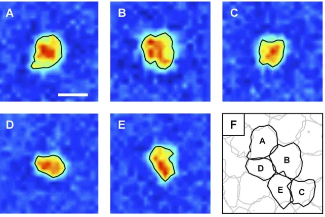
under-of visual space that will be mapped by such neuron. As stated before, the retinal output –result of a series of integrations across the different cell types– is ultimately generated by the ganglion cells, thus usually one will speak of the receptive field of a ganglion cell when referring to a retinal receptive field. Classically, RFs were considered circular, and eventually ellipsoidal. Today, this approximation is still used for the geometric simplicity it implies. However, real RFs vary substantially from this description [58]. In fact, they have a fine structure and irregular contours that differ from cell to cell, where neighbors complement each other, as it would happen in a puzzle, meaning that the cell population is spatially coordinated (Figure 1.5) [58].
Figure 1.5: Receptive fields with irregular shapes, which allow for a more uniform mapping of the visual space. Image taken from [58].
Another important point about receptive fields is that they usually follow an antagonist center/surround organization. These antagonists are simply called ON and OFF. This
part does the opposite, i.e., responds to negative changes in intensity (diminishing). So, while considering that the center will allow for the maximum activation of the neuron, we can conclude that, e.g., an ON-center/OFF-surround cell will fire the most when only its center receives light. If both center and surround receive light, the neuron will not fire as much; while with no light at all, or light only on the OFF-surround part, the cell will not fire at all. Here, firing means eliciting a spike-train, or simply generating the electrical signal we have been discussing previously. Now, we are ready to enlarge our knowledge of ganglion cells.
1.2.2 Standard ganglion cells
Ganglion cells are the output of the retina. For many years, scientists only observed what now are called standard ganglion cells. This classification is given to midget and parasol ganglion cells, who respectively provide information for detailed perception, and action.
Midget ganglion cells represent around 70%-80% of the ganglion cells’ population [38][115]. They analyze and provide to the rest of the system information of details and high-frequency high-contrast in central vision. They are also sensitive to color, and have slower conduction velocity compared to the parasol cells.
Parasol ganglion cells represent around 10% of the ganglion cells’ population [38][115]. They analyze and provide to the rest of the system motion information, low-frequency low-contrast, and information from flashing objects. Differently to midget cells, parasol cells are insensitive to color, and are faster than midget cells to propagate their output.
1.2.3 Non-standard ganglion cells
Noticed later than their standard counterparts by the scientific community, non-standard ganglion cells are considered to be older in the phylogenesis [70], and to provide information for detection [70][107].
This detection, however, is rough but fast, and focuses on events or particular objects. Its goal is to induce survival-oriented actions on time [91], and to drive higher-level iterative processes with prior information [15][86].
Non-standard cells have been found to participate in blind-sight, i.e., where “clinically blind” patients report being unable to consciously perceive visual stimuli, yet they are able
When compared to standard cells, non-standard cells –such as small bistratified gan-glion cells– account for about 10% of the gangan-glion cells’ population [71][84]. Despite the notorious difference in proportion against the midget cells, parasol and bistratfied cells map the entire visual field thanks to larger receptive fields [189][58]. Here, Figure 1.6 shows us the dendritic morphology of ganglion cells in the macaque, and their receptive fields follow this fashion in terms of size.
Figure 1.6: Dendritic morphology of macaque ganglion cells. Parasol and bistratified ganglion cells compensate for their reduced amount, compared to midget cells, with larger receptive fields. Image taken from [39].
temporal pattern recognition on their own [62, 184]. This includes motion detection, direc-tional selectivity, local edge detection, object motion and looming detection [107][62][184]. Nevertheless, the reliability of the detection is relatively low –it is difficult to identify com-plex patterns with a single and large RF– and it will have generally to be confirmed by a subsequent analysis with smaller and more numerous RFs of the standard pathway. These different functions could have developed over time, as researchers have found that during phylogenetical evolution, the eye was not a simple feedforward system: Feedback informa-tion from the remainder of the nervous system had been able to produce adaptive learning of sophisticated visual functions to “optimize the transfer of information” [160]. These capabilities could have evolved to the point of now being pre-wired, i.e. existent without any need for adaptation.
In a nutshell, non-standard cells provide fast, a priori event detection assumptions to the remainder of the visual system [91].
1.2.4 Projections of ganglion cells: The birth of visual pathways
Besides the standard and non-standard classification, we can group retinal outputs in streams, which is a notion we will use for the rest of this document. Under this scheme, we will have the Parvocellular [16], Magnocellular [16] and Koniocellular [70] pathways. These pathways start with, and keep the properties of, the information produced by midget, para-sol and non-standard ganglion cells, respectively. They receive their names from different neurons in the thalamus, which we will discuss later.
An overview of the retinal projections and the pathways being born with them is shown in Figure 1.7.
Just as a reminder, midget cells and the Parvo pathway carry information for per-ception, while parasol cells and the Magno pathway carry information for action, and non-standard cells and the Konio pathway carry information for detection. This is the key difference between these three classes, and summarizes well their role throughout the whole visual system.
Before we review the thalamus, let us describe the stage right above, the cortex, so we can later easily discuss the thalamocortical aspects and interactions.
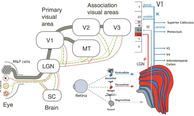
Figure 1.7: Different retinal projections. (Left) Midget and parasol projections are shown in black, while different non-standard channels are depicted in colors. Image taken from [107]. (Right) Projections to the lateral geniculate nucleus (LGN) and thereafter. Again we observe the widespread connectivity of Konio cells, that receive information from bis-tratified ganglion cells. Image modified from [115].
1.3
The major processing power of our visual system is kept in the cortex. Like a large distributed mainframe, the visual cortex computes information to be used by several struc-tures at the same time, building distributed interpretations/representations of the world, that are to be composed in higher cognitive levels. For the purposes of this document, we will focus on the earliest stage of the visual cortex: the primary visual cortex (V1) [18].
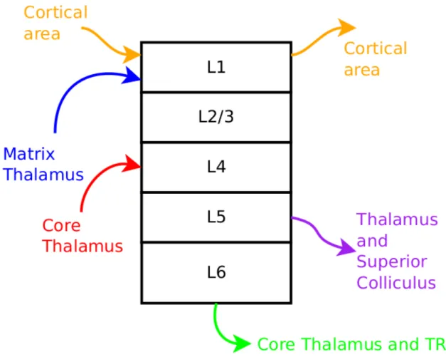
V1 is tiled with elementary and repeated neuronal circuits that authors call the cor-tical column [74]. It is basically a layered structure made by 6 levels, usually grouped as superficial (composed by layers 1, 2 and 3 upper), middle (3 lower and 4), and deep (5 and 6) layers. Figure 1.8 depicts it in a simplified manner. Here, it is shown that superficial layers receive information from other cortical areas and the matrix thalamus, in order to modulate information processing in the column, respectively, towards a stimulus expected from cortical inference or roughly detected from the non-standard pathway. Middle layers receive precise sensory information from the core thalamus, and with the information from cortical expectation and thalamic modulation, the output will be produced and commu-nicated through the deep layers towards the thalamus as feedback, and to motor regions, like the superior colliculus.
As shown in Figure 1.7, V1 receives feedforward information coming from the thalamus –which will be described in the next section– from all three visual pathways. In addition, it receives information from other cortical areas.
A summary of the anatomical circuitry and their functions in the early thalamocortical loops of mammals –used to validate the thalamocortical connections used in our model– is represented in Table 1.1, adapted from [124] and [67].
In the introduction to this chapter, we mentioned the “what” (perception) and the “where/how” (preparation for action) pathways [63]. The “what” pathway, also called temporal –or ventral– stream, is involved with object identification. After layer 4Cβ in V1, information goes through areas V2, V3, V4 and on, towards IT. At the same time, the “where/how” pathway, also called parietal –or dorsal– stream, is involved with self-referenced localization (i.e. with oneself as point of reference). After layer 4Cα in V1, information goes through areas V2, V3, V5/MT and on, towards MST and FEF. All these links, pathways, and their interactions, serve to integrate information and achieve more and more developed processing at each higher stage.
Figure 1.8: Simplified cortical column. Here, only a handful of information flows are represented, just to give an idea of the interactions of the cortical column with other structures. TRN stands for thalamic reticular nucleus, and core and matrix thalamic structures are explained in section 1.4.1. The superficial layers receive information from other cortical areas and the matrix thalamus, in order to modulate or bias processing in the column towards an expected, or unexpected, stimulus, respectively. Middle layers receive information from the core thalamus, and with the information from cortical expectation and thalamic modulation, the output will be produced and communicated through the deep layers towards the thalamus as feedback, and to motor regions, like the superior colliculus.
Table 1.1: Anatomical circuitry and functions of V1 connections.
Model connections Type Functional interpretation References First order core thalamic cells
→ layer 4 cells of V1
D Primary thalamic relay cells drive layer 4
[10]
First order core thalamic cells → layer 6(1) cells of V1
D Primary core thalamic cells prime layer 4 via the 6→4 modulatory circuit [10] for LGN→6; LGN input to layer 6 is weak [15]; Layer 5 projects to 6 [Note1]
First order core thalamic cells → TRN
D Recurrent inhibition to core thalamus
[152][82]
TRN → First order core thala-mic cells
I Inhibition of primary and secondary core thalamic cells, synchronization of core thalamic cells
[152]
TRN → TRN I Normalization of inhibition [157][82]
TRN → TRN GJ Synchronize TRN and
tha-lamic relay cells
[94]
TRN → Matrix thalamic cells I Inhibition of matrix thala-mic cells
[87][173]
Matrix thalamic cells → Layer 5 cells of V1
M To layer 5 through apical dendrites in layer 1
[173]
Layer 4 cells of V1 → Layer 4 inhibitory interneurons of V1
D Lateral inhibition in layer 4 [103]
Layer 4 inhibitory interneurons of V1 → Layer 4 cells of V1
I Lateral inhibition in layer 4 [103]
Layer 4 inhibitory cells of V1 → Layer 4 inhibitory interneurons of V1
I Normalization of inhibition in layer 4
Model connections Type Functional interpretation References Layer 4 cells of V1 → Layer 2/3
cells of V1
D Feedforward driving out-put from layer 4 to layer 2/3
[50][17]
Layer 2/3 cells of V1 → Layer 2/3 cells of V1
D Recurrent connections in layer 2/3
[11][142][124]
Layer 2/3 cells of V1 → Layer 2/3 inhibitory interneurons of V1
D Avoid outward spreading in layer 2/3
[112][124]
Layer 2/3 inhibitory cells of V1 → Layer 2/3 inhibitory in-terneurons of V1
I Normalization of inhibition [163][124]
Layer 2/3 cells of V1 → Layer 4 cells of V2
D Feedforward information [175]
Layer 2/3 cells of V1 → Layer 6(2) cells of V2
D Feedforward information [175]
Layer 2/3 cells of V1 → Layer 5 cells of V1
D Conveys output from layer 2/3 to layer 5
[17]
Layer 2/3 cells of V1 → Layer 6(2) cells of V1
D Conveys output from layer 2/3 to layer 6(2)
[15]
Layer 5 cells of V1 → Pulvinar D Feedforward information to V2 through the pulvinar
[152]
Layer 5 cells of V1 → Layer 6(1) cells of V1
D Delivers corticocortical feedback to the 6(1) → 4 circuit from higher cortical areas, sensed at the apical dendrites of layer 5 cells branching in layer 1
[15][17][Note 2]
Layer 6(1) cells of V1 → Layer 4 cells of V1
M Excitation fo layer 4 [161][15][124]
Layer 6(1) cells of V1 → Layer 4 inhibitory interneurons of V1
Model connections Type Functional interpretation References Layer 6(2) cells of V1 → LGN M Direct feedback
informa-tion to LGN
[156][15]
Layer 6(2) cells of V1 → TRN D Indirect feedback to LGN, to be used by TRN in order to regulate LGN
[68][152]
Layer 6(2) cells of V2 → Layer 5 cells of V1 → Layer 6(2) cells of V1 → Layer 4 cells of V1
M Intercortical feedback from layer 6(2) of V2 to layer 1 of V1, where it synapses on layer 5 cells because their apical dendrites branch in layer 1, resulting in sublim-inar priming of layer 4 cells via the “layer 5 to layer 6(1) to layer 4” circuit
[131][140]
Table 1.2: Summary of anatomical circuitry of early thalamocortical loops of mammals Abbreviations: D = driving connections; M = modulatory connections; I = inhibitory connections; GJ = gap junctions. [Note 1] [15] subdivides neurons in layer 6 in 3 classes: Class I: project to 4C, also receive input from LGN, and project to LGN; Class IIa: dendrites in layer 6, receive projections from 2/3, project back to 2/3 with modulatory connections; Class IIb: dendrites in 5, project exclusively to deep layers (5 and 6) and claustrum. Here, these populations are clustered in 2 classes, layer 6(1) and 6(2), which provide feedback to thalamic relay cells and layer 4, respectively. [Note 2]: [15] ubdivides Layer 5 neurons in 3 classes: Class A: dendrites in 5, axons from 2/3, project back to 2/3 with modulatory connections; Class B: dendrites in 5, axons from 2/3, project laterally to 5 and the pulvinar; Class C: dendrites in 1, project to SC. Here, layer 5 neurons receive input from 2/3 (Classes A and B), as well modulatory input from nonspecific thalamic nucleus (Class C, apical dendrites in layer 1), and provides output to layer 6(1) and the pulvinar.
the “slower what” and the “faster how” streams, where the prior focuses in hierarchical processing (i.e. sequential), and the latter on preparing action processing (with a more parallel processing). These streams focus on the interpretation of the visual scene, where a hypothesis is developed by grouping information from the different receptive fields in order to “make sense of the environment” (see Figure 1.9). This process of binding information in the current hypothesis is another way to look at what a cortical expectation is. A cortical expectation is a certain information “predicted” by the cortex, and “expected” to be there, or to happen. An example would be for us to expect to see a ball that is thrown moving in a more or less straight line, rather than to see it moving like a serpent during its flight.
1.4
The thalamus: The collaborative harmonizer
The thalamus [146] is a structure in charge of regulating the information flow to cortical areas. It is located between the cortex and the midbrain, and communicates with several cortical and extra-cortical areas, including peripheral structures, such as the retina. It is thanks to all these connections, and what it does with them, that we call it a collaborative harmonizer.
The thalamus is composed by different clusters of neurons, each one called a thalamic nucleus. Figure 1.10 shows an overview of thalamic nuclei, while Figure 1.11 is a schematic of their different connections. From these nuclei –and in the scope of the present document– the most important are the lateral geniculate nucleus (LGN), the pulvinar, and the thalamic reticular nucleus (TRN).
To give a brief first idea: from a functional point of view [115], LGN works like a smart relay of retinal information, while the pulvinar does something similar with cortical information. TRN, however, will not relay any information and instead will regulate –by inhibiting the thalamus– the thalamocortical flows from, and to, LGN and the pulvinar.
Another important fact is that the thalamus will allow for a “current thalamocortical hypothesis” to exist. This is nothing else than the current information being processed, that is formed thanks to the feedforward flows. The feedforward hypothesis will be corrected through feedback information, particularly the one coming from expectations and goals (cf. Section 1.4.1).
? ?
? ? ? ? 1 4 5 1 ~ ~ ~ ~
Figure 1.9: Integration of information through thalamocortical and cortico-cortical interactions This figure represents a simplification of the interaction between information flows, i.e. the interplay between feedforward and feedback information, to-gether with local receptive field integration, and expectation corrections done through higher-level receptive fields. Left: The upper rectangle represents a higher-level unit (of V2, here), where the lines and the ellipse represent its receptive field, that consider 3 cells of a lower-level structure (of V1, here). Two of these cells identify a horizontal stimulus, while we delay the processing of the cell in between them to show how receptive fields, feedforward information, and expectation, work to define the output of a certain unit by integration. This delay could also be interpreted as uncertainty due to noisy or inconsistent signal. Here, this middle unit can identify 4 types of orientation, as represented by the lines in the smaller squares. Middle: The cell locally evaluates the preferred orientation, scoring the largest for a diagonal, being this the local feedforward hypothesis. However, it is de-picted in the upper box that the higher-level unit, by grouping, has established a straight horizontal line as stimulus, and thus the expectation information (cf. Section 1.4.1), rep-resented by the descending link, will force the unit to be “corrected” and ponder higher the horizontal line, despite the local score, and because of its global, higher-level, analysis. Right: The scores are no longer considered, and the units are in synchrony analyzing a horizontal line.
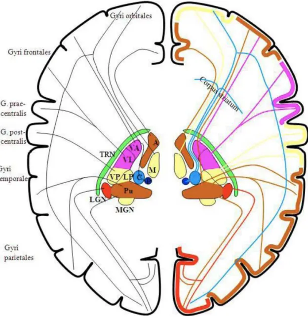
Figure 1.10: Overview of thalamic nuclei. Here, A1 is the primary auditory cortex, S1 is the primary somatosensory cortex, VA is the ventral anterior nucleus, VL is the ventral lateral nucleus, DL is the dorsal lateral nucleus, LP is the lateral posterior nucleus, VPL is the ventral posterolateral nucleus, and VPM is the ventral posteromedial nucleus. Image taken from [64].
Figure 1.11: Thalamocortical connections and how TRN is involved. Here we see how TRN sort of wraps (like a plastic protection for a sandwich) the thalamic nuclei, receiving collaterals from both thalamus and cortex, and harmonizing these flows via inhibitory actions at the thalamic level. Image taken from [114].
1.4.1 Properties of thalamic structures
In order to better characterize thalamic nuclei, one must be first aware of the jargon used to describe them. Here, we will discuss their classification by order (first/higher order)[153], types of cells (core and matrix)[80][81], what their activation modes are (tonic/burst)[154], and how connectivity allows us to label their outputs (as driver or modulator)[154]. In addition, we will discuss the “no strong loops” hypothesis for thalamic (and cortical) pro-jections.
First and higher-order nuclei
When we talk about order, we simply mean “what input”. This makes first-order equal to peripheral, like we see with LGN receiving input from the retina, and higher-order equal cortical, like we see with the pulvinar receiving input from the primary visual cortex (V1) and other cortical regions.
Core and matrix cells
When we talk about core or matrix cells, we look at “where and how it outputs”. The reason for having only two names rather than four is that cells project in only two ways. The first one, used by core cells, consists in projecting topographically to middle cortical layers (3 lower and 4), which is called the “precise” way. The second one, used by matrix cells, consists in projecting non-topographically to upper cortical layers (1, 2, 3 upper), and it is called the “diffuse” way. In addition, this diffuse way also considers other areas in the cortex.
Core cells produce driving flows, while matrix cells produce modulating flows (cf. Sec-tion 2.1.2).
Tonic and burst modes
The information transmission modes of thalamic neurons were first studied in slow-wave sleep [148]. Here, bursting was of major interest, where scientists observed these sustained rhythmic bursts across large cell populations, where the firing was synchronized. The first observations showed that bursting prevented the normal function of the cells, which at the time was considered only to be relaying information, through the tonic mode. However, in awake activities, a thalamic neuron will transmit information in tonic and burst mode
and thus it is considered that sensory information is transmitted via this mode. On the other hand, the burst mode is the non-linear transmission mode, where bursts improve the signal-to-noise ratio, and are thus thought of allowing the capture of new information.
These modes are supposed to be generated because of intrinsic properties of the thala-mic neurons. Particularly, because of calcium (Ca2+) conductances in their T-type calcium channels. A T-type calcium channel is a low-voltage activated “tunnel” that allows for a calcium influx to enter a cell after a spike or a depolarizing signal. Here, depolarization is when the membrane potential of the cell becomes “more positive” or “less negative”, while its conductance is a mathematical parameter representing the ease of electric cur-rent flow through this channel. So, these modes happen thanks to a threshold: when a cell is relatively depolarized for 100ms or more, T-type calcium channels are inactivated, thus allowing cells to fire in tonic mode. However, when a cell is relatively hyperpolarized (opposite of depolarized) for 100ms or more, T-type calcium channels are activated, and provoke the burst mode, where 2 to 10 spikes are generated per burst. Here, the excitatory cortical input (from layer 6) promotes tonic firing, while the inhibitory input from TRN promotes burst firing [104].
Our interpretation is that the burst mode comes in handy when looking for something new. This “something new” is linked to cortical expectations.
When cortical expectations are not met, we call it a mismatch. In order to say whether there is such mismatch, or not, feedforward information must be compared to the expec-tations, reflected by feedback information. This task is topographically carried out by TRN –receiving feedforward and feedback flows to compare reality against expectation–, who possesses inhibitory capabilities to regulate thalamic nuclei. In the case TRN resolves that there is no mismatch, sensory information can be transmitted through tonic mode. However, in the case of a mismatch, the burst mode is needed to improve the SNR, and to either validate cortical expectations by realizing that the mismatch is not as great as previously computed, or to allow for a topographically wider search in the information, as the SNR increase would provoke a larger inhibition in the mismatching regions, allowing for this search elsewhere in the topographic map.
Driver and modulator information flows
structure. An example would be the output of core cells in the LGN towards layer 4 of V1. This information flow alone triggers cortical responses, altogether with being considered for first-order thalamocortical mismatch. A modulator, on the other hand, is unable to trigger a response by itself on the receiving structure, and instead will regulate (modulate) what is already being analyzed. An example would be the output of matrix cells in the LGN towards layer 1 of V1. This information flow will help to regulate, or empower (being excitatory), certain regions, but will not be directly responsible for the output, and will not be considered for the first-order thalamocortical mistmatch.
All this could be put in situation : driver information from the lateral geniculate nucleus, e.g. encoded in the Magno pathway, will be transmitted in tonic mode unless the thalamic reticular nucleus sends a modulating mismatch signal, which would require to block (maximal inhibition) the feedforward flow, switch to burst mode, and allow for a search elsewhere than the current focus point (or a new interpretation).
The “no strong loops” hypothesis
This hypothesis for thalamic and cortical projection establishes that there shall be no loops created only with driving information flows, as the consequence of having one would be uncontrolled cortical oscillations [35]. This hypothesis arises from graph theory, where the mathematical theory of directed graphs, or digraphs, is used. A digraph is a series of nodes (and in our case, thalamocortical structures) connected by lines, where each line shows the direction of the information transmission with an arrow. Here, if a digraph has a directed loop (i.e. loop with only driving information flows, in our case), then it is not possible to generate a hierarchy of levels. On the other hand, if there is no directed loop, the nodes (structures) can form a hierarchy, but it may not be a unique one.
In our case, this simply means that a stable system should not have such loops, and the early visual system does not contain any so far [35].
1.4.2 The complex relay: the lateral geniculate nucleus
LGN, or the lateral geniculate nucleus, is a first-order nuclei, composed by both core and matrix cells. In primates, it is composed by 6 main layers, where intralaminar structures are found between them. In layers 1 and 2 we localize Magno-cells, in layers 3-6 the Parvo-cells, and Konio cells are present in the intralaminar structures. The core part of LGN is
and saw that these cells gave birth to the Parvo, Magno, and Konio pathways. Taking this into account, it is not surprising that the different cells in LGN share many properties of their retinal counterparts (cf. Figure 1.7):
• The Parvo cells carry slow and sustained neuronal activity for layer 4Cβ of V1 con-cerning color and shapes.
• The Magno cells carry rapid and transient information for layer 4Cα of V1 concerning motion, brightness and depth.
• The Konio cells process different kinds of non-standard information and project to upper layers in the cortex. The next section is dedicated to them.
In addition, core LGN receives strong cortical feedback from layer 6 of V1, together with a degree of inhibition from TRN. All these can be seen in Figure 1.12. This, we interpret, as a result of the mismatch between feedforward and feedback information (expectation).
1.4.3 Konio pathway and its projections
The Konio stream, or non-standard pathway, is here considered as “for detection”. This raw, coarse, a-priori detection of visual events is done by integrating information from groups of non-standard retinal ganglion cells. The results of this detection can allow for survival actions to be done promptly [91], and also to drive higher-level processes with prior information [15].
Here, the Konio pathway is considered to be a quick pathway. This consideration does not arise from its processing speed, as we will see in the last section of this chapter, but instead from the reduced number of hops when compared with its Parvo and Magno counterparts.
There are 5-6 classes of Konio axons2 afferent to V1. However, they seem to be orga-nized in 3 Konio streams [24][70]:
• The dorsal Konio layer, that carries low acuity information and projects toward layer 1 of V1.
• The middle Konio layer, that carries information from central blue cones to layer 3B of V1.
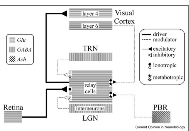
Figure 1.12: Schematic diagram of circuitry for the lateral geniculate nucleus The inputs to relay cells are shown along with the relevant neurotransmitters and postsynaptic receptors (ionotropic and metabotropic) Abbreviations: Ach, acetylcholine; GABA, γ-aminobutyric acid; Glu, glutamate; LGN, lateral geniculate nucleus; PBR, parabrachial region; TRN, thalamic reticular nucleus. Image and caption taken from [149].
![Figure 1.1: Gross architecture of the early visual system. Image taken from [69], itself adapted, with permission from [59].](https://thumb-eu.123doks.com/thumbv2/123doknet/14238689.486437/33.918.259.655.219.724/figure-gross-architecture-early-visual-image-adapted-permission.webp)